Full-Spectrum LED-Driven Underwater Spectral Detection System and Its Applications

Abstract

Spectral detection technology offers non-destructive, in situ, and high-speed capabilities, making it widely applicable for detecting biological and chemical samples and quantifying their concentrations. Water resources, essential to life on Earth, are widely distributed across the planet. The application of spectral technology to underwater environments is useful for wide-area water resource monitoring. Although spectral detection technology is well-established, its underwater application presents challenges, including waterproof housing design, power supply, and data transmission, which limit widespread application of underwater spectral detection. Furthermore, underwater spectral detection necessitates the development of compatible computational methods for sample classification or regression analysis. Focusing on underwater spectral detection, this work involved the construction of a suitable hardware system. A compact spectrometer and LEDs (400 nm–800 nm) were employed as the detection and light source modules, respectively, resulting in a compact system architecture. Extensive tests confirmed that the miniaturized design-maintained system performance. Further, this study addressed the estimation of total phosphorus (TP) concentration in water using spectral data. Samples with varying TP concentrations were prepared and calibrated against standard detection instruments. Subsequently, classification algorithms applied to the acquired spectral data enabled the in situ underwater determination of TP concentration in these samples. This work demonstrates the feasibility of underwater spectral detection for future in situ, high-speed monitoring of aquatic biochemical indicators. In the future, after adding UV LED light source, more water quality parameter information can be obtained.

1. Introduction

Spectral detection is a widely utilized technique with numerous applications in environmental monitoring, biomedicine, and industry [1,2,3]. Spectral technology is fundamentally composed of detection hardware modules and analytical algorithms. The hardware module typically consists of a spectrometer, a light source, and associated optical fixtures. The selection of wavelength bands for the light source and spectrometer is closely linked to the specific application. For example, in environmental monitoring, the visible to near-infrared (400–1100 nm) spectrum enables accurate detection of chlorophyll’s characteristic absorption peak at 683 nm, as well as the scattering behavior of suspended solids in the 550–700 nm range [4]. In biomedical applications, the ultraviolet (UV) band (200–400 nm) enables DNA quantification through the characteristic absorption of nucleic acids at 260 nm [5], while the NIR band (700–2500 nm) is used for non-invasive imaging by leveraging the optical windows of tissues at 850 nm and 970 nm [6].

For industrial inspection, the mid-infrared (2500–25,000 nm) can identify the C-H stretching vibration of polyethylene at 2915 cm⁻¹ and the C=O characteristic peak of polycarbonate at 1770 cm⁻¹ [7]. Agricultural remote sensing particularly focuses on the red-edge band (680–750 nm), assessing nitrogen status by monitoring the red-edge shift in wheat at 720 nm, or determining the extent of pest and disease infestation in rice using reflectance characteristics at 700 nm [8,9]. Astronomical observations select wavebands based on the characteristics of different celestial bodies, ranging from observing Lyα radiation of young stars in the UV band to studying the thermal radiation of interstellar dust in the far-infrared [10,11]. Spectral bands are chosen based on the specific responses of target substances, reflecting the core principle of wavelength selection driven by material properties.

Conventional underwater spectral detection systems often rely on halogen lamps or xenon lamps as light sources, which provide wide spectral coverage but suffer from high power consumption, bulky structures, and complex waterproof packaging requirements, limiting their portability and long-term in situ applications [12]. In contrast, the compact full-spectrum LED adopted in this work offers broad and continuous emission with high luminous stability and energy efficiency, enabling integration into a miniaturized detection system suitable for field deployment. Furthermore, while classical regression algorithms such as Partial Least Squares Regression (PLSR) and Principal Component Regression (PCR) are widely used for spectral quantitative analysis, they often show limited capability in addressing non-linear spectral–concentration relationships [13]. Recent advances in machine learning and deep learning have demonstrated improved predictive accuracy in water quality monitoring tasks by leveraging Gaussian Process Regression (GPR) and Convolutional Neural Networks (CNNs), which provide automatic feature extraction and robust performance against noise [14]. Building upon these developments, our study combines an optimized hardware design with advanced regression algorithms, representing a novel approach for accurate, compact, and energy-efficient underwater spectral sensing.

Underwater spectral monitoring faces unique challenges; due to the strong selective absorption of light by water molecules, it is essential to carefully select operational wavebands to obtain effective signals. UV-green light band is typically chosen as the primary operational band. Studies indicate that the UV band (200–400 nm) is particularly suitable for tracking chromophore dissolved organic matter (CDOM), owing to its significant characteristic absorption by aromatic compounds at 260–280 nm [15,16].

In clear waters, the blue light band (450–490 nm) can sensitively capture the strong absorption valley of chlorophyll a in phytoplankton at 443 nm. Conversely, when the water is turbid, the green light band (490–580 nm) exhibits stronger penetration, effectively monitoring the scattering characteristics of suspended sediments in nearshore waters around 550 nm [17,18,19,20]. This precise “band-component” matching enables underwater spectral technology to overcome the difficulties of water attenuation and successfully achieve quantitative retrieval of different aquatic environmental parameters [21,22,23].

The primary applications of spectral data are material classification and quantitative analysis. In situations where high precision is not required, discretized quantitative analysis can also be achieved through classification algorithms. In spectral data material classification, various machine learning algorithms exhibit distinct characteristics. Support Vector Machines (SVMs), by employing kernel tricks to map data into high-dimensional feature spaces, construct an optimal classification hyperplane based on the principle of structural risk minimization [24,25,26]. Their unique “margin maximization” characteristic renders them highly effective in water quality classification with limited samples, such as algae identification. Deep Extreme Learning Machines (DELMs) innovatively integrate the feature abstraction capabilities of deep neural networks with the rapid computational advantages of ELM [27,28,29]. For example, in coral reef spectral classification, their deep architecture can automatically extract characteristic absorption peaks at 580 nm while maintaining training speeds at the second level.

Furthermore, Random Forest algorithms, by constructing multiple decision trees and employing Bagging ensemble strategies, can not only effectively handle high-dimensional spectral data (e.g., NIR spectra containing 2000 bands) but also output wavelength importance rankings (e.g., identifying the 720 nm feature as most critical for shipwreck relic identification). Convolutional Neural Networks (CNNs) leverage their local receptive field characteristic to automatically capture feature patterns in spectral curves (e.g., absorption abruptions of crude oil contamination at 420 nm) [30,31,32,33]. However, their performance is highly dependent on the scale of training data, typically requiring thousands of calibrated samples to achieve ideal results. Collectively, these algorithms constitute a powerful toolkit for intelligent underwater spectral analysis.

In spectral quantitative analysis, various regression algorithms demonstrate their unique advantages. Partial Least Squares Regression (PLSR) effectively addresses the challenge of high correlation between wavelengths [34] by ingeniously projecting both spectral data and concentration data into a latent variable space, though its modeling relies on representative calibration samples. Principal Component Regression (PCR), which first employs PCA for spectral dimensionality reduction (e.g., compressing 2000 bands to 10 principal components), simplifies the model structure but may risk losing critical feature information (e.g., neglecting the weak characteristic peak of dissolved organic matter at 515 nm). Neural Network Regression (e.g., BPNN), with its powerful non-linear fitting capabilities, can accurately characterize complex spectral-concentration relationships (e.g., synergistic absorption effects of mixed heavy metal ion pollutants), but requires careful network architecture design and regularization techniques to prevent overfitting. These methods provide diverse solutions for underwater spectral quantitative analysis with varying precision requirements.

This study focuses on underwater spectral detection and the corresponding quantitative analysis of chemical substances. Given that over 70% of the Earth’s surface is covered by water, the monitoring and protection of water resources represent a significant research objective. However, the development of compact underwater spectrometers is currently limited. This is primarily due to the challenges associated with underwater monitoring, which necessitates the waterproof installation of opto-mechatronic components and the detection of water samples through an optical window, typically made of glass. Such requirements impose stringent demands on system compactness and stability. For instance, spectral probes must have a sufficient working distance to monitor water in its natural environment through an optical window, and light sources, along with their power drivers, must be compact yet provide high luminous output. It should be noted that although in situ detection is innovative, its implementation remains challenging and is affected by many factors. Chemical methods are still the most accurate. However, optical in situ detection can provide early warnings, simply by providing preliminary concentration information, which can aid in water quality monitoring and protection.

In this work, Light Emitting Diodes (LEDs) were chosen as the light source for underwater spectral detection. In recent years, the improving luminous efficiency and stability of LEDs have made them a preferred light source for numerous optical detection applications. Concurrently, the emergence of LEDs emitting at specific wavelengths offers potential for water quality monitoring. For example, LEDs in the 230–250 nm band are crucial light sources for nitrogen compound detection. Although such LEDs are not yet commercially off-the-shelf, they are being investigated as custom components in industrial applications. It is anticipated that in the near future, 230–250 nm LEDs will become standard, providing an important light source for online water quality monitoring.

Compared to conventional LEDs used for general illumination, full-spectrum LEDs, which approximate the solar spectrum, are gradually gaining prominence in the lighting field. They provide a broad and continuous range of wavelengths, enabling more accurate and comprehensive analysis of target materials. Their compact size and energy efficiency make them ideal for integration into underwater spectral detection devices. Based on this background, the present work employs a full-spectrum LED, combined with a compact spectrometer and a stable industrial camera, to achieve online underwater monitoring. Additionally, the proposed system has a wider range of application scenarios. We developed an inversion model for the water-quality parameters and realized the visualization of total phosphorus, which can better assess eutrophication fundamentally. Consequently, our instrument can continue monitoring and analyzing the water quality, promote the harmonious growth of the ecological environment, and bring economic benefits.

Spectral-based total phosphorus analysis has been widely studied, and the classic total phosphorus detection is analyzed using a wide spectral band. In order to verify the effectiveness of the underwater spectral detection instrument, this work selected a wide spectral band to carry out the analysis of total phosphorus.

For example, a study in the literature [35] points out that using 400–900 nm spectral data and back propagation neural network (BP) to build TP inversion models. Zhang et al. successfully retrieved TP concentrations in Baiyangdian Lake using hyperspectral reflectance relying on 400–1000 nm bands [36]. Similarly, Dong et al. also applied hyperspectral modeling to predict TP levels in inland waters, highlighting the effectiveness of full-spectrum regression rather than single-band analysis [37].

2. Materials and Methods

2.1. Design and Characterization of the Underwater Spectral Detection System

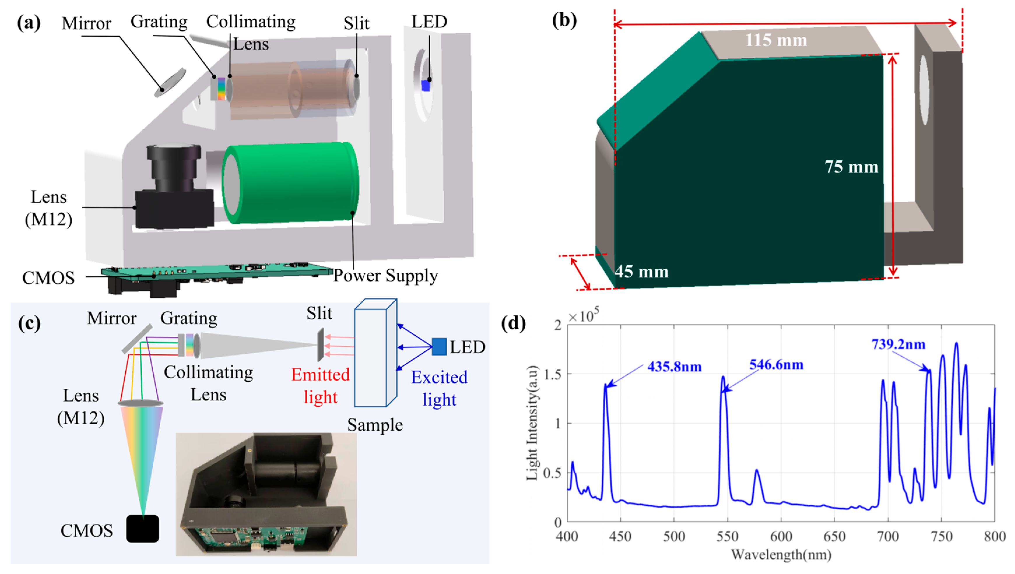
To reduce the size of the spectrometer, this study employed a transmission grating as the dispersive element to construct a compact spectral detection module. As illustrated in Figure 1, the spectrometer system was designed with overall dimensions of 105 mm × 75 mm × 45 mm (Figure 1b). The three-dimensional model (Figure 1a) details the arrangement of its primary components, which include a slit, an achromatic lens, the transmission grating, an imaging lens, an LED, a CMOS sensor, the power supply, and a control board. In a classical spectrometer, the slit is the key component to provide spectral resolution and is the entrance pupil of the spectrometer. The smaller the width of the spectrometer slit, the better its spectral resolution. For underwater spectral detection, a spectrometer resolution of about 5 nm is sufficient. Therefore, we chose a 50-micron slit, and the spectral resolution of the entire system is 8 nm. An industrial CMOS camera AR0130, characterized by its high operational stability across a wide temperature range, was utilized to collect the spectral signals. The goal of this work is to construct a miniaturized spectrometer, so the dimensions of the optical components in the spectrometer are customized. The slit has a diameter of 12 mm, and the diameter of the doublet lens behind the slit is 11 mm, with a focal length of 45 mm. Doublet lenses offer better chromatic aberration correction than single lenses. In this work, we used a transmission grating with 300 line pairs/mm whose blaze wavelength is approximately 500 nm. Preceding the slit, a 45 mm focal length achromatic lens is used to gather the transmitted light from the water sample through a 5 mm thick glass window. This window thickness is sufficient to withstand water pressure at a depth of 50 m, and the 45 mm focal length achromatic lens ensures efficient collection of optical signals from the water sample, while also maintaining high spectral resolution. In order to reduce the size, the system uses a silver-coated mirror to fold the optical path. The diameter of the silver-coated mirror is 20 mm. At the same time, the CMOS sensor is customized as a rectangular structure, and its longer side is parallel to the light splitting path. The sensitive wavelength of AR0130 CMOS sensor (1280 × 960 resolution, 3.75 μm Pixel Size, 8-bit output) is 400–1000 nm. In front of the CMOS sensor, there is an M12 lens with a focal length of 50 mm. The CMOS sensor and the STM32 microcontroller transmit data via the DCMI interface. The microcontroller’s serial port can also control the exposure time and gain of the CMOS sensor. Details of CMOS sensors can be found in Reference [38]. In this way, the compactness of the system can be better guaranteed. We used this system to obtain the spectrum of a standard mercury argon lamp, whose peak wavelength was consistent with the wavelength of the standard light source.

Because of the high efficiency of spectral detection, we selected a low-power LED. For scenarios involving weaker signals, high-power LEDs, also available in compact structures, could be chosen, further underscoring the significant potential of LEDs in underwater detection. A full-spectrum LED (emission range: 400 nm–800 nm) was selected to illuminate the water sample. This LED can be driven by a 3.3 V supply, eliminating the need for complex linear or switching power supplies, and exhibited good light intensity stability even at this standard voltage, adequate for water body spectral detection. The assembled system underwent pressure testing and was confirmed to operate normally at a depth of 50 m without leakage. The CMOS camera consumes 500 mA at 12 V, acquiring spectral signals with a high signal-to-noise ratio at this voltage.

To reduce power consumption during extended underwater operation, the system adopts a sleep strategy based on the Stop mode. This allows the device to enter a low-power state during periods of communication inactivity or in the absence of control commands, with the CPU and main system clock disabled while UART wake-up capability remains active. In this configuration, the system can be reactivated via a Bluetooth command transmitted through the UART interface. Static current is lowered from 30–40 mA to approximately 300–600 μA, helping to extend battery life. To balance responsiveness and energy efficiency, the system includes communication timeout detection and a minimum sleep duration threshold to avoid unnecessary mode transitions. This approach is suitable for low-duty-cycle, energy-aware underwater sensing tasks, providing consistent support for spectral data acquisition.

We also evaluated the system’s dark noise, spectral resolution, and repeatability. It is noteworthy that although the industrial camera has an 8-bit depth, by leveraging the low distortion characteristics of the imaging spectrometer, the two-dimensional spectral image captured by the CMOS can be converted into one-dimensional spectral data. Without requiring image correction, the resulting dynamic range of the data is between 0 and 255. A detection system with a high dynamic range provides high-quality data for subsequent quantitative analysis.

2.2. Characterization of the Full-Spectrum LED Light Source and Its Suitability for the Underwater Spectral Detection System

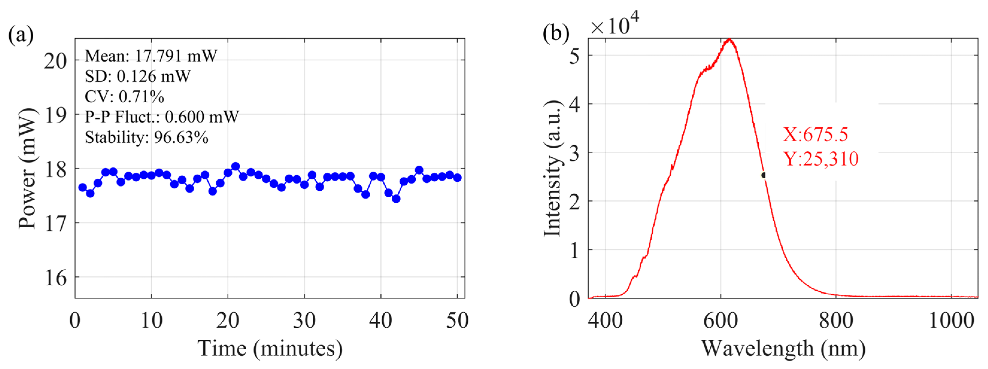
To assess the suitability of the selected full-spectrum light-emitting diode (LED) as the light source for the underwater spectral detection system, particularly for the estimation of total phosphorus (TP) concentration in water, its key operational characteristics were evaluated. The temporal stability of the LED’s power output was monitored over a 50-min duration, with measurements taken at 1-min intervals, as depicted in Figure 2a. The LED demonstrated robust stability, exhibiting a mean power output of 17.791 mW. Fluctuations were minimal, characterized by a standard deviation of 0.126 mW and a coefficient of variation (CV) of only 0.71%. The peak-to-peak power fluctuation observed during the measurement period was 0.050 mW, corresponding to a relative stability of 96.63%, which indicates consistent illumination suitable for precise and in situ measurements of parameters like total phosphorus in wide-area water resource monitoring. The emission spectrum of the LED, presented in Figure 2b, reveals a primary emission peak centered at approximately 614 nm with spectral width spanning from 450 nm to 800 nm. This broad and continuous spectral output, covering the visible to near-infrared range, confirms its spectral properties are appropriate for the effective detection of total phosphorus and other biochemical indicators in underwater environments. These results confirm the full-spectrum LED’s high stability and suitable spectral properties for its intended use in the compact underwater spectral detection system developed in this study, demonstrating the feasibility of future in situ, high-speed monitoring of aquatic biochemical indicators.

2.3. Sample Preparation and Experimental Measurement

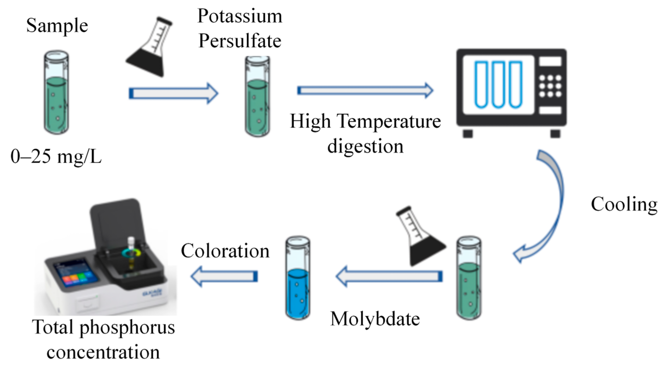
In order to verify the effectiveness of the system, we choose standard measuring instruments as the gold standard. At the same time, water samples with different concentrations were constructed in this work for modeling and testing. The water samples for testing were collected from Dongpo Lake at Hainan University. Prior to spectral measurement, the original water samples were diluted with deionized water to prepare 12 different total phosphorus (TP) concentration gradients. For each concentration, samples were placed in a sealed sampling chamber, and their absorption spectral data were captured using the underwater spectrometer. A total of 120 spectral datasets were obtained. Concurrently, to obtain precise standard values for the TP content of each diluted sample, measurements were performed using a multi-parameter water quality analyzer (Model: GL930, Brand: GLKRUI), following the ammonium molybdate spectrophotometric method. These measurements from the GL930 analyzer served as the gold standard or ‘true values’ for the total phosphorus concentration, which were subsequently used to train and validate the predictive models developed in this study. This procedure involved digesting the water samples under high temperature and pressure to convert all forms of phosphorus into orthophosphate. Subsequently, the orthophosphate reacted with molybdate reagent and was developed with a reducing agent for colorimetric determination. Finally, the absorbance was measured at a specific wavelength using the instrument’s photometer and converted to TP concentration. To ensure the reliability of the standard values, each concentration group was measured 10 times. The experimental workflow is illustrated in Figure 3.

2.4. Spectral Data Pre-Processing

Raw spectral data acquired by the system can exhibit characteristics such as high dimensionality, band redundancy, and the presence of instrument noise. Therefore, appropriate pre-processing steps are essential to mitigate these effects, remove artifacts, and enhance the quality of the data for subsequent quantitative analysis.

Firstly, the collected raw hyperspectral data $I_{raw0}$ from the water samples underwent normalization. In this system, the LED light passes through L = 1.67 cm water medium before entering the spectrometer slit and being detected. Since the water absorption coefficient varies greatly in the visible-near-infrared spectrum, the difference in water absorption ${\mu }_a\left(\mathsf{\lambda }\right)$ will affect the spectral detection. Therefore, after obtaining the original spectrum, this paper uses the Beer–Lambert formula to correct for water absorption by $I_{raw}=I_{raw0}/exp\left({\mu }_a\right(\mathsf{\lambda }\left)\mathrm{L}\right)$.

This crucial step aimed to correct for variations due to dark current and any non-uniform spectral response originating from the illumination system or detector. The normalization procedure utilized a standard white reference panel spectrum $I_{white}$ and a dark spectrum $I_{dark}$, which was captured with the LED light source turned off. The raw spectral data were converted into normalized reflectance $I_{ref}$ using the following equation:

$$I_{ref}={\displaystyle \frac{I_{raw}-I_{dark}}{I_{white}-I_{dark}}}$$

(1)

Secondly, even after normalization, the reflectance spectra $I_{ref}$ can be affected by residual instrumental and environmental noise, which can degrade data quality and impact analytical outcomes. To address this, a smoothing procedure was applied to the normalized reflectance data. In this study, the Savitzky–Golay smoothing algorithm was employed. This algorithm fits a polynomial function to data points within a defined moving window and uses the value of the fitted polynomial at the center of the window as the new, smoothed data point. The Savitzky–Golay method is effective in reducing random errors and high-frequency fluctuations while generally preserving the essential shape, width, and higher-order derivative information of the underlying spectral signals.

The pre-processed spectra resulting from these preprocessing steps (i.e., the smoothed normalized reflectance, $I_{ref}$ were then used as the primary input for the various machine learning models developed for total phosphorus quantification, as detailed in Section 3. For clarity and consistency with the descriptions in Section 3, these pre-processed spectra are subsequently referred to as ‘absorption spectra’ within the context of the modeling work presented in this paper.

3. Results

3.1. Quantitative Inversion of Total Phosphorus Concentration Using an Artificial Neural Network

For the quantitative inversion of total phosphorus (TP) concentration in water samples, this study employed an Artificial Neural Network (ANN) model. ANNs are powerful machine learning models capable of learning complex non-linear relationships between input features and target variables.

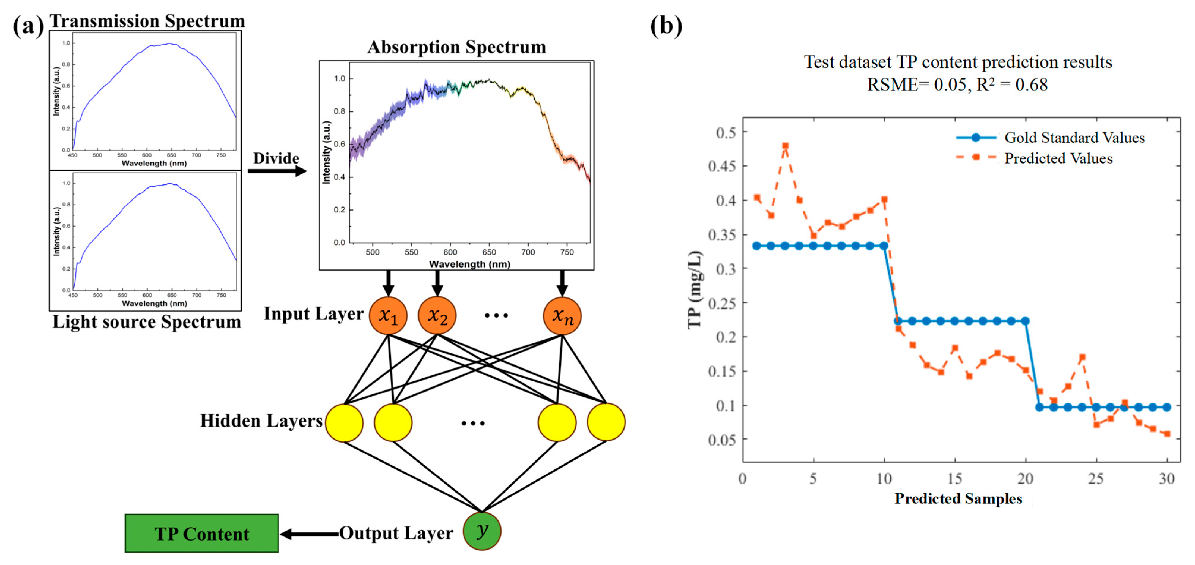
The input features for the ANN were derived from pre-processed hyperspectral data. Following initial data pre-processing steps, including normalization and Savitzky–Golay smoothing (as previously described or in Section 2.4), “absorption spectra” were calculated. This was achieved by dividing the processed water quality spectra by the corresponding light source spectra for each sample. These derived absorption spectra, along with the laboratory-measured TP concentrations, formed the dataset for model development. The experiment included water samples with varying TP concentrations; for instance, twelve of the samples, whose original hyperspectral data were subsequently processed into absorption spectra, had TP concentrations of 0.51, 0.44, 0.33, 0.27, 0.22, 0.189, 0.147, 0.119, 0.097, 0.078, 0.07, and 0.053 mg/L.

The dataset, consisting of 12 distinct concentration groups, was partitioned to ensure a rigorous and unbiased evaluation of the models. Specifically, nine of these concentration groups were randomly selected to form the training set, which was used for model learning. The remaining three concentration groups were designated as the testing set for independent performance evaluation. Crucially, the data from this testing set were not used at any stage of the model training process. Input data were organized as a matrix where rows represented samples and columns represented spectral features (bands). An ANN with a specific architecture was designed, featuring an input layer, two hidden layers with 10 and 5 neurons, respectively, and an output layer predicting TP concentration. To mitigate the impact of varying scales among different spectral features and improve training stability, the input absorption spectra data underwent standardization before being introduced to the network. To provide a comprehensive evaluation, we assessed model performance using three key metrics: the coefficient of determination (R²) to measure the proportion of variance explained, the root means square error (RMSE) to quantify the magnitude of prediction errors, and the mean bias error (Bias) to identify any systematic tendency for over- or under-estimation.

The ANN was trained by iteratively adjusting its internal parameters (weights and biases) to minimize the discrepancy between its predictions and the actual TP values in the training data. The predictive performance of the trained ANN model was rigorously assessed on the unseen testing set. The model yielded a coefficient of determination (R²) of 0.68, a root mean square error (RMSE) of 0.060 mg/L, and a Bias of −0.006 mg/L, indicating a slight tendency to underestimate the TP concentration. Figure 4a provides a schematic overview of the entire process, including the derivation of absorption spectra from water quality and light source spectra, and the subsequent input into the defined ANN architecture. A comparison between the TP concentrations predicted by the ANN model and the gold standard values (measured by the GL930 analyzer) for the test samples is presented in Figure 4b. This scatterplot directly compares the system’s performance with that of the gold standard instrument on the test data.

3.2. TP Concentration Prediction Performance of Machine Learning Algorithms

Among the methods evaluated, Gaussian Process Regression (GPR) was investigated. GPR, a non-parametric machine learning technique grounded in Bayesian theory, defines a prior Gaussian process over functions and calculates the posterior distribution based on observed data to achieve regression prediction. The experimental data comprised the same pre-processed hyperspectral absorption spectra (derived from transmittance data as described in Section 3.1) and corresponding laboratory-measured TP concentrations. These absorption spectra served as input features for the model, with TP concentration as the prediction target. The dataset was partitioned into training and testing sets using the same splits employed for the ANN, with the majority of samples utilized for model training and the remainder reserved for rigorous performance validation. Input data were structured in a [number of samples × number of features (bands)] format. The GPR model was implemented using the fit function in MATLAB, employing a constant basis function and a squared exponential kernel function to construct the covariance matrix. To mitigate the influence of varying scales among different spectral features, the input data underwent standardization pre-processing. During the training phase, kernel function hyperparameters were optimized using maximum likelihood estimation.

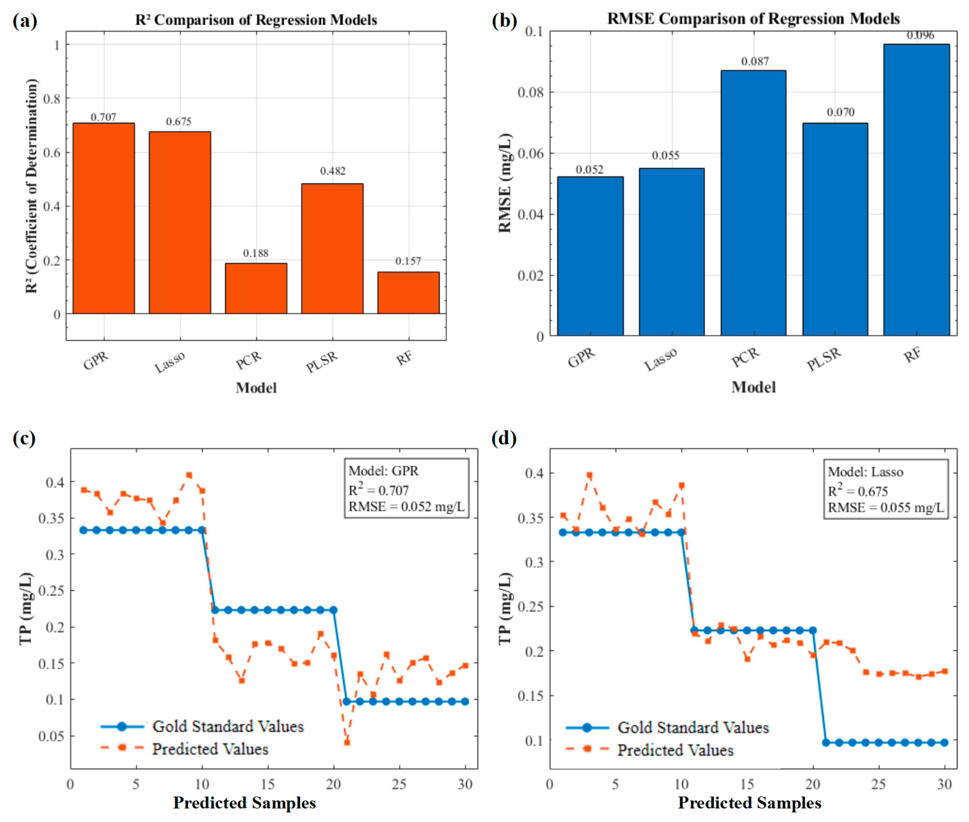
The GPR model demonstrated significantly improved predictive capability on the test set, achieving a coefficient of determination (R²) of 0.7065 and a root mean square error (RMSE) of 0.0522 mg/L. Furthermore, it exhibited a small positive Bias of 0.0057 mg/L, indicating a very slight tendency to overestimate the TP concentration. A comparison between the TP concentrations predicted by the GPR model and the actual measured values is illustrated in Figure 5c. To further assess the GPR model’s robustness and highlight its advantages for this TP inversion task, its performance was systematically compared with several other established regression algorithms. These included Random Forest (RF), Partial Least Squares Regression (PLSR), Principal Component Regression (PCR), and Lasso regression. All models were trained and tested on the identical data partitions and pre-processed spectral data. For the Partial Least Squares Regression (PLSR) and Principal Component Regression (PCR) models, the optimal number of latent variables (components), a critical hyperparameter, was determined using a rigorous 10-fold cross-validation procedure on the training set. We evaluated a range of components from 1 to 20 and selected the number that minimized the root mean square error of cross-validation. This data-driven approach ensures that each model was tuned to its optimal capacity for a fair and robust comparison.

The comparative analysis, with R² values summarized in Figure 5a and RMSE values in Figure 5b, revealed that the GPR model exhibited superior performance. Lasso regression achieved the second-best results, with an R² of 0.6752 and an RMSE of 0.0550 mg/L; its Bias was 0.0331 mg/L, also showing a tendency to overestimate the concentration. PLSR demonstrated moderate efficacy (R² = 0.4786, RMSE = 0.0696 mg/L, Bias = 0.0192 mg/L). In contrast, both RF (R² = 0.0836, RMSE = 0.0923 mg/L, Bias = 0.0303 mg/L) and PCR (R² = 0.1883, RMSE = 0.0869 mg/L, Bias = 0.0272 mg/L) showed significantly lower predictive accuracy on this dataset. The superior performance of GPR in this context can be attributed to several factors. Its non-parametric nature allows it to flexibly model complex, non-linear relationships within the hyperspectral data without pre-specifying the functional form. The Bayesian framework provides a principled approach to uncertainty quantification and hyperparameter optimization, enhancing robustness, particularly with potentially limited datasets. The squared exponential kernel is adept at capturing smooth functions, which may characterize the relationship between the processed spectral features and TP concentration. Lasso regression also performed commendably, largely due to its inherent feature selection capability through L1 regularization. Hyperspectral data are often high-dimensional and exhibit multicollinearity. Lasso’s ability to shrink some coefficients to zero effectively selects a subset of the most relevant spectral bands. This reduces model complexity, mitigates overfitting, and can improve generalization, especially when many features are noisy or redundant.

These findings underscore the enhanced capability of the GPR model, closely followed by Lasso regression, in accurately quantifying TP concentration from hyperspectral data. The Bias analysis provides further confirmation: while all models exhibited a positive Bias, indicating a tendency to overestimate TP concentration, GPR’s systematic error was the lowest. Combining the lowest error magnitude (RMSE) with the least systematic bias solidifies its standing as the most reliable and suitable model for this application.

In contrast, the traditional chemometric models—PLSR and particularly PCR—exhibited significantly poorer performance even after optimization. This underperformance highlights a fundamental limitation of applying linear methods to what is evidently a complex, non-linear relationship. PCR’s low accuracy is attributable to its modeling strategy, which selects principal components to capture maximum variance in the spectral data (X) without regard for their correlation to the TP concentration (Y). Consequently, it risks retaining noise-heavy components while discarding lower-variance components crucial for prediction. While PLSR performed better by selecting latent variables based on covariance, its inherent linearity still constrained its predictive power. The clear inadequacy of these optimized linear models strongly justifies the application of more advanced, non-linear approaches like GPR for this task.

3.3. Total Phosphorus Prediction Using a Convolutional Neural Network

However, the performance of GPR models is highly dependent on the choice of kernel function, and their feature extraction capabilities may be limited when dealing with high-dimensional, complex non-linear spectral data. To further enhance prediction accuracy and leverage the advantages of deep learning models in automatic feature extraction and complex pattern recognition, this study subsequently constructed and optimized a Convolutional Neural Network (CNN) regression model.

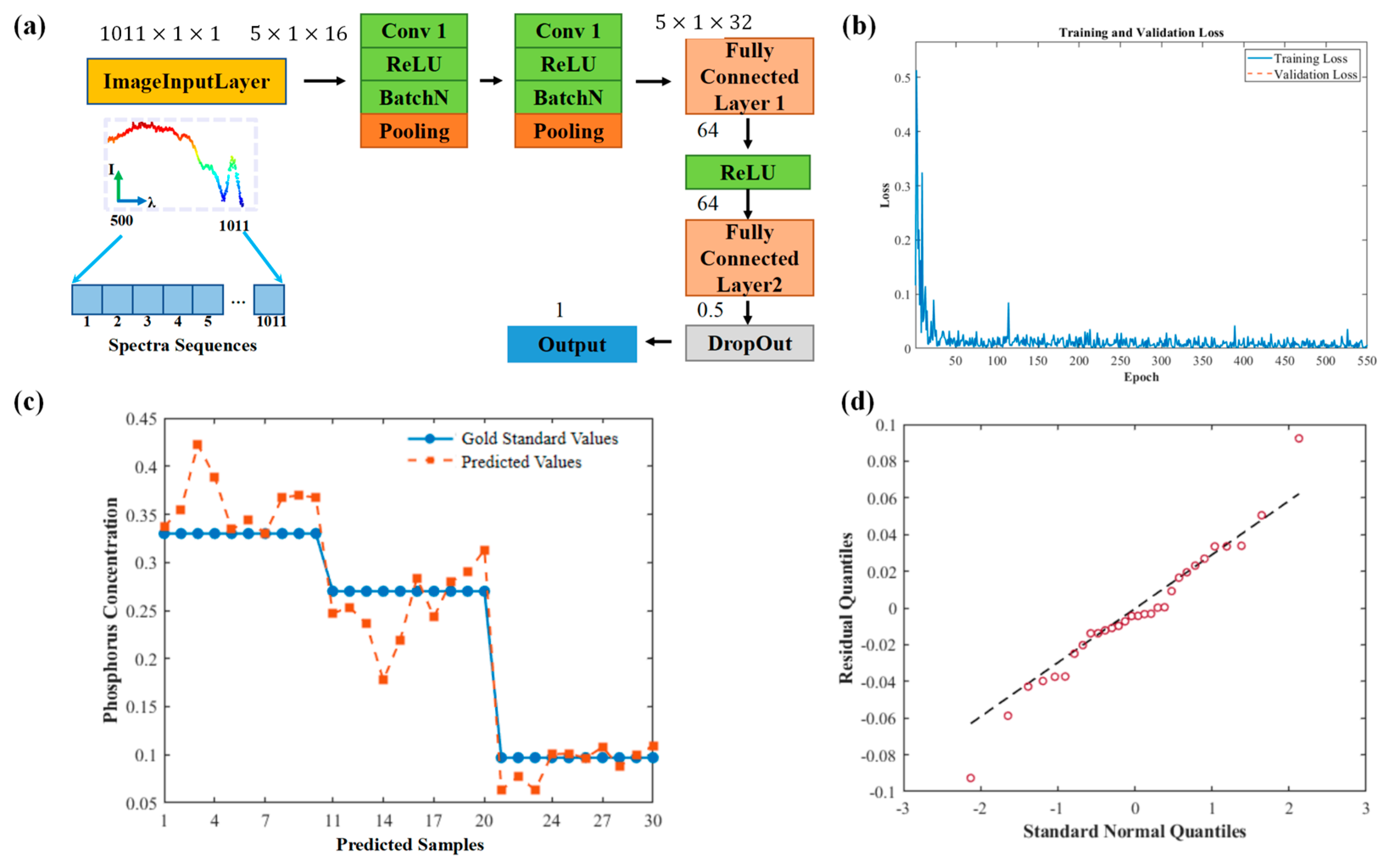
The CNN model, the architecture of which is depicted in Figure 6a, was specifically designed to process one-dimensional absorption spectral data, aiming to directly learn discriminative features from the raw spectra, thereby overcoming the limitations of manual feature engineering. Its input is a single-channel spectral sequence (dimension 1011 × 1), and the output is a scalar value representing the phosphorus concentration. The network architecture was designed considering the characteristics of spectral data: after the input layer receives the spectral signal, the first one-dimensional convolutional layer (configured with 16 filters of size 1 × 5, using a ‘same’ padding strategy) extracts local spectral features. One-dimensional convolution was chosen as spectral data are inherently one-dimensional sequences; the 1 × 5 filter size aims to capture local correlations between adjacent bands (such as the edges or slopes of absorption peaks), while ‘same’ padding ensures that the feature map size remains unchanged, preventing the loss of edge information. This is followed by Batch Normalization to accelerate training convergence, improve model stability, and provide a degree of regularization. Subsequently, a ReLU non-linear activation function is applied to introduce non-linear expressive power, enabling the network to learn more complex functional relationships efficiently. This is followed by a 1 × 2 max-pooling layer, which achieves feature dimensionality reduction by selecting the maximum value in local regions, thereby reducing computational load while retaining the most salient features and imparting some invariance to minor spectral shifts. The second convolutional layer (configured with 32 filters of size 1 × 5) further mines higher-order, more abstract spectral patterns; the number of filters was increased (from 16 to 32) to enable the network to learn a richer set of feature representations, accompanied by the same batch normalization, ReLU activation, and 1 × 2 max-pooling operations. The feature map, after pooling, is flattened to convert the two-dimensional feature map into a one-dimensional vector, suitable for input to fully connected layers. It is then fed into a fully connected layer containing 64 nodes, which integrates and recombines the previously extracted distributed features, further learning non-linear combinations between them, also using a ReLU activation function. To effectively mitigate potential overfitting on the limited dataset, a dropout regularization technique with a rate of 50% was introduced. Finally, a single-node fully connected layer (with linear activation) outputs the predicted total phosphorus concentration value, directly corresponding to the regression task’s target. Compared to GPR, the main advantages of the CNN lie in its end-to-end learning capability and hierarchical feature extraction mechanism. It can automatically learn effective features related to TP concentration from raw spectral data without requiring predefined complex feature engineering steps. Its multi-layer structure allows for hierarchical abstraction from low-level local spectral details (e.g., absorption intensity at specific wavelengths) to high-level composite features (e.g., relative relationships of multiple absorption bands), potentially capturing complex spectral-concentration mapping relationships that GPR models with fixed kernel functions might struggle to identify.

The CNN model was trained using the Adam optimizer for a total of 250 epochs, with an initial learning rate set to 1 × 10⁻³ and a batch size of 16. To monitor the training process and make timely adjustments, model performance was evaluated every 10 epochs on a validation set containing samples with specific concentrations (0.33, 0.27, 0.097 mg/L). The learning progression, including training and validation loss curves, is presented in Figure 6b, which helps in assessing convergence and identifying potential overfitting. All model construction, training, and evaluation were performed within the MATLAB 2021a Deep Learning framework. GPU acceleration was not enabled for this experiment, and the complete training process for the CNN model took approximately 2 min.

Through this detailed structural design and parameter optimization, the CNN model demonstrated a significant performance improvement. As shown in Figure 6c, which compares the predicted and actual values on the test set, the model achieved a coefficient of determination (R²) of 0.87 and a root mean square error (RMSE) reduced to 0.03 mg/L. The calculated mean bias error (Bias) was −0.0208 mg/L, indicating a slight systematic tendency to underestimate the TP concentration. This indicates its higher accuracy and robustness in the quantitative inversion of total phosphorus concentration in water bodies. Furthermore, a Quantile–Quantile (Q-Q) plot of the model residuals was generated to assess their normality (Figure 6d). The Q-Q plot demonstrates that the residual quantiles align closely with the theoretical quantiles of a standard normal distribution, indicating a relatively uniform distribution of residuals that approximates normality. This supports the statistical validity of the model’s error structure and the reliability of the aforementioned performance metrics.

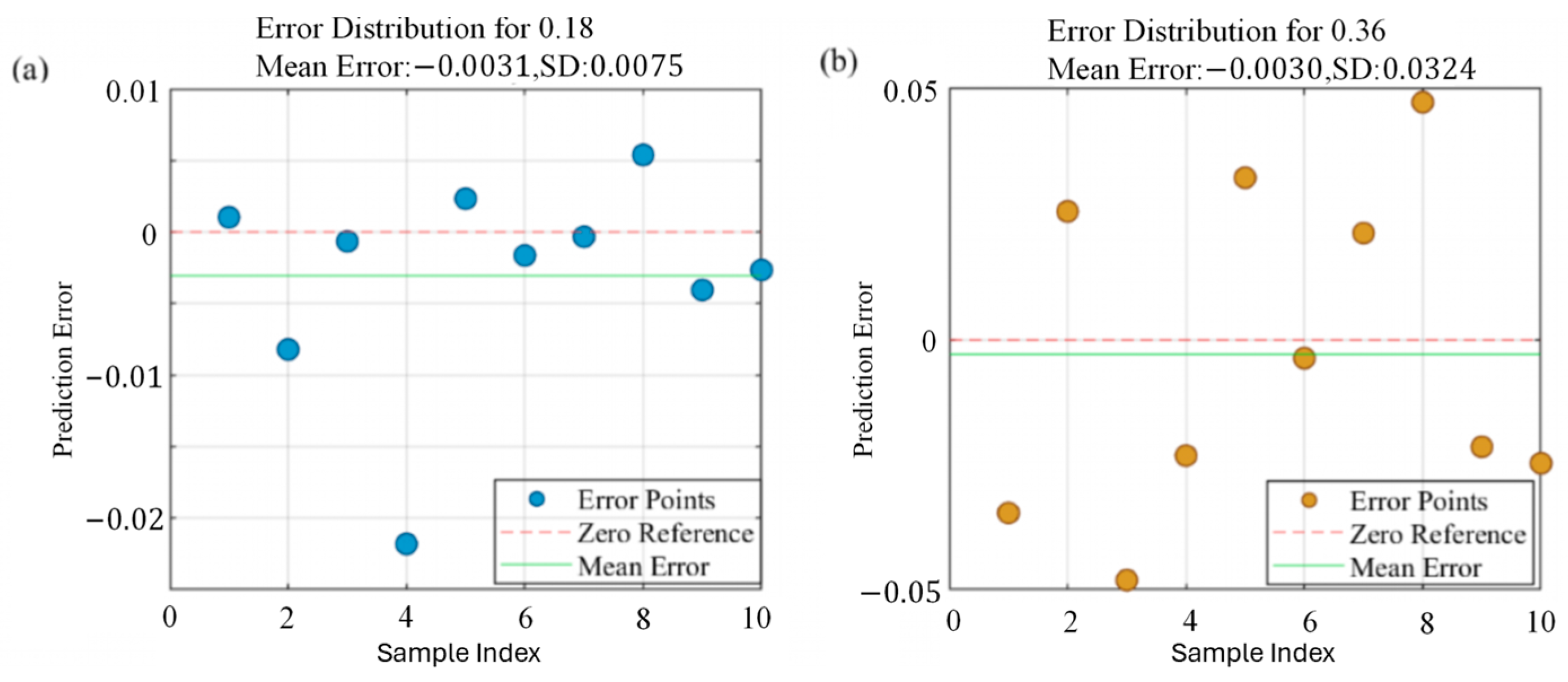
To provide a final, more rigorous test of the model’s practical generalization, specifically its capacity to interpolate between the discrete concentration levels used in training, an additional validation was conducted. We used real water samples with TP concentrations of 0.14 mg/L and 0.32 mg/L, which represent intermediate values not present in the original 12-group dataset. As shown in Figure 7, the model performed strongly, with mean relative errors of 3.43% and 8.82%, respectively. This result confirms the model’s robustness and underscores its suitability for real-world deployment where it will encounter a continuous range of concentrations.

Additional experiments were conducted to verify the rationality of the selected 400–800 nm spectral range by comparing the predictive performance of a model trained on the full band versus one trained on a truncated 500–800 nm band.

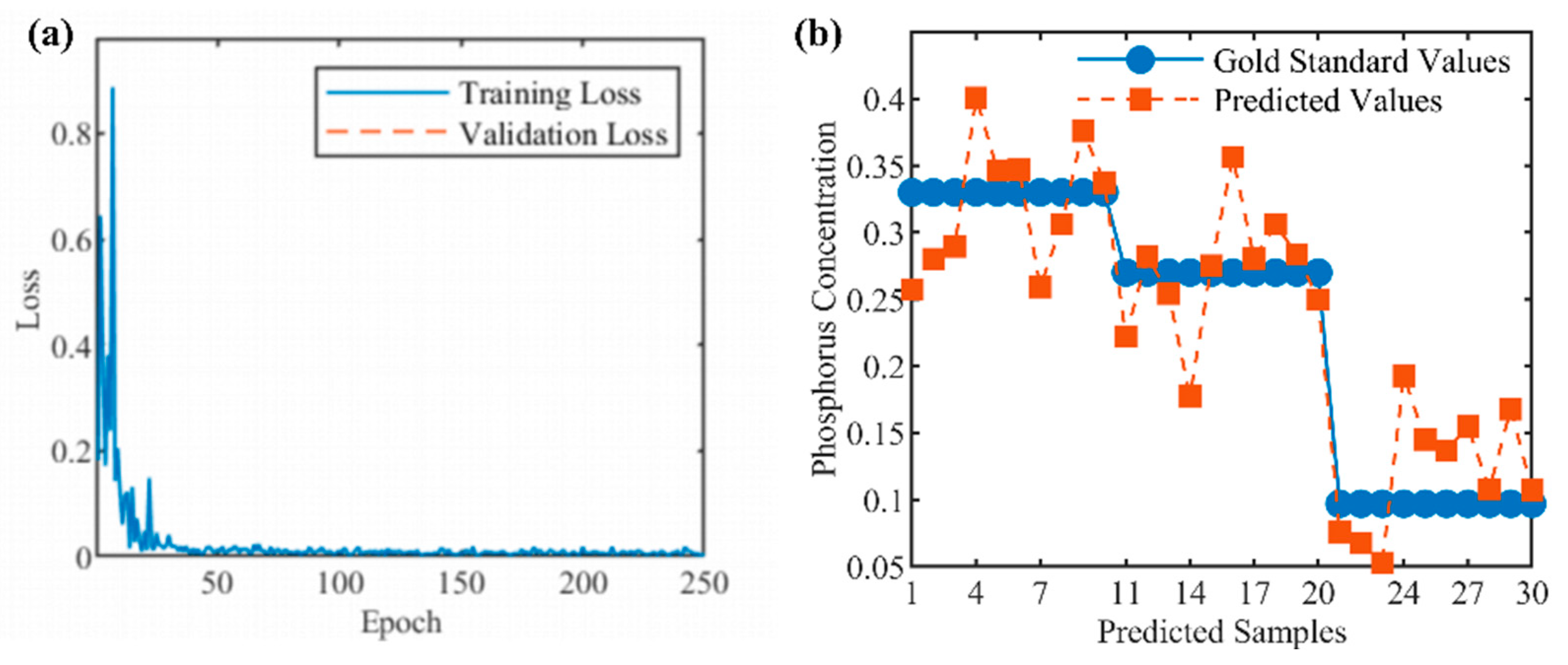
The 2D-CNN model was constructed using reflection spectrum data from the 500–800 nm band. As shown in Figure 8a, the training and validation losses showed a stable decrease and eventually converged, indicating that the model training was effective and without significant overfitting. Figure 8b shows the model’s predictive performance on the test set. The resulting accuracy metrics (R² = 0.72, RMSE = 0.048 mg/L) indicated that there was still room for improvement when compared to the full-band model (R² = 0.87, RMSE = 0.03 mg/L). This comparison demonstrates that although the 500–800 nm band model has basic usable performance, the full-band model exhibits superior comprehensive performance in both prediction accuracy and error distribution control.

4. Conclusions

This study successfully details the development, characterization, and application of a compact, full-spectrum LED-driven underwater spectral detection system designed for quantitative analysis. The custom-engineered system, incorporating a transmission grating spectrometer and a robust housing, demonstrated reliable operation, including stability at a 50-m depth, and the capability to acquire high-quality hyperspectral data (e.g., effectively utilized in the 400–800 nm range after pre-processing) suitable for complex chemical analysis. A primary application focused on the quantitative determination of total phosphorus (TP) concentration in water samples. The acquired spectral data, subjected to normalization and Savitzky–Golay smoothing, served as input for various machine learning models. Initial investigations with an Artificial Neural Network (ANN) provided a baseline performance (R² = 0.68, RMSE = 0.060 mg/L, Bias = −0.006 mg/L). Subsequent evaluation of several established regression algorithms revealed that Gaussian Process Regression (GPR) offered significantly improved predictive accuracy (R² = 0.7065, RMSE = 0.0522 mg/L, Bias = 0.0057 mg/L), outperforming Random Forest, PLSR, PCR, and Lasso regression in this specific application. To further advance predictive performance and leverage automated feature extraction, a one-dimensional Convolutional Neural Network (CNN) was specifically designed and optimized for TP quantification from the spectral data. The CNN model demonstrated markedly superior results, achieving an excellent coefficient of determination (R²) of 0.87 and a low root mean square error (RMSE) of 0.03 mg/L, and a bias of −0.0208 mg/L on the test set. This result highlights the CNN’s superior ability to extract complex spectral patterns, enabling more accurate and robust predictions.

Using diluted samples from real lake water, we prepared 12 concentration levels, which are sufficient for early warning monitoring. We used regression analysis, and because the 12 concentrations are discrete, the final regression analysis results present a categorical outcome. However, this method, in essence, utilizes regression analysis, and it is sufficient for monitoring and early warning of abnormal total phosphorus levels in water.

In the research on miniaturization of spectrometers, current researchers mainly focus on the miniaturization of spectrometers themselves. However, in many applications, light sources are also necessary. Compact and broad-spectrum LED light sources can significantly reduce the size and power consumption of the entire system, improving portability and integration. As far as we know, LEDs with spectral bands ranging from 350 nm to 1000 nm are already being developed. This wideband, miniaturized LED light source is highly valuable for the miniaturization of spectrometers. The findings underscore the considerable potential of combining compact, LED-based underwater spectral sensing technology with advanced deep learning models like CNNs for effective, rapid, and precise in situ monitoring of crucial biochemical parameters such as total phosphorus. This research paves the way for the development of more portable, efficient, and intelligent underwater spectral systems, holding promise for diverse applications in water resource management, environmental protection, and real-time aquatic ecosystem assessment.