Neural Network Robustness Analysis Using Sensor Simulations for a Graphene-Based Semiconductor Gas Sensor ^†

Abstract

Despite their advantages regarding production costs and flexibility, chemiresistive gas sensors often show drawbacks in reproducibility, signal drift and ageing. As pattern recognition algorithms, such as neural networks, are operating on top of raw sensor signals, assessing the impact of these technological drawbacks on the prediction performance is essential for ensuring a suitable measuring accuracy. In this work, we propose a characterization scheme to analyze the robustness of different machine learning models for a chemiresistive gas sensor based on a sensor simulation model. Our investigations are structured into four separate studies: in three studies, the impact of different sensor instabilities on the concentration prediction performance of the algorithms is investigated, including sensor-to-sensor variations, sensor drift and sensor ageing. In a further study, the explainability of the machine learning models is analyzed by applying a state-of-the-art feature ranking method called SHAP. Our results show the feasibility of model-based algorithm testing and substantiate the need for the thorough characterization of chemiresistive sensor algorithms before sensor deployment in order to ensure robust measurement performance.

1. Introduction

Chemiresistive gas sensors are important technologies for environmental monitoring and other application fields since they combine advantages in their cost of production with their flexibility [1]. In its basic form, such a sensor device consists of a sensing layer, which molecules in the air can adsorb onto or desorb from. Adsorption and desorption processes have a direct impact on the electrical properties of the sensing layer, such as its resistivity/conductance [2]. These properties are measured and combined with suitable pattern recognition algorithms in order to translate them into either a classification guess or a concentration estimate [3].

The development process of such sensors typically involves the thorough characterization of the sensor material and the analysis of its hardware components. The characterization of the functional materials can involve spectroscopic techniques [4,5], such as X-Ray Diffraction, as demonstrated for a tin-oxide material by Kim et al. [6], or Raman spectroscopy, such as that investigated for a graphene-based material by Travan et al. [7]. Apart from the material properties themselves, other components of the sensor are also analyzed. As chemiresistive gas sensors mostly include microheaters [8], there has been a large effort in characterizing the heating properties, such as the temperature distribution on the material, by means of FEM, for example [9,10]. The results obtained by the described characterization procedures can help to develop models for the studied sensor. This is usually achieved by fitting experimental measurements to the model equations, taking the material-specific effects derived from the characterization into consideration [11,12,13,14].

Despite the availability of a number of techniques for the characterization of hardware components, only a few studies on such techniques have been proposed regarding focusing on the characterization of the algorithms responsible for gas prediction. Moreover, the available studies that provide an analysis of algorithm characteristics, such as their robustness to different sensor instabilities, tend to focus on standardized techniques, such as Principal Component Analysis (PCA) or Linear Discriminant Analysis (LDA) [15,16]. The above-mentioned methods are the standard choice when it comes to proving and assessing the separability performance of new sensing materials [17,18,19,20]. Nevertheless, algorithms for chemiresistive gas sensors have progressed over the years and neural networks have become more common in the field of environmental monitoring [21,22,23,24]. As a consequence, a literature gap has arisen on techniques to assess and explain the validity of these more complex and less transparent models in terms of their robustness.

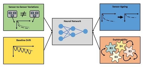
In this work, we aim at characterizing smart chemiresistive gas sensors from a new perspective. Instead of analyzing the sensor material or its hardware, we thoroughly characterize the algorithms operating on top of the sensors. The main focus of our investigations lies on the explainability of these algorithms, as well as their robustness to the different instabilities that prototypical technologies typically entail. The goal is to provide a full evaluation scheme for different algorithm types and for chemiresistive gas sensors by adopting a system-level simulator previously developed for the investigated sensor device. Our main contributions are:

• The investigation of a state-of-the-art feature ranking method and its usefulness to make neural network algorithms for chemiresistive gas sensors explainable.
• The study and the quantification of the impact of sensor-to-sensor variations at the production stage on the performance of a set of different machine learning algorithms.
• An analysis of the performance degradation of different prediction algorithms in the presence of multiplicative and additive baseline drift.
• An examination of the effect of chemiresistive sensor ageing and its impact on algorithm accuracy.

The experimental evidence of our contributions is structured into four different studies. Each of the studies contains an additional overview of the related work in the specific area in the Materials and Methods section. The studies share the same data configuration in terms of concentration profiles, which is provided by a simulation model of a graphene-based chemiresistive gas sensor that we developed in previous research [14,25]. Furthermore, the techniques that we present throughout this paper are designed to be model-agnostic, which means that they are also applicable for other pattern recognition algorithms, which are not part of our study setup.

The structure of our paper is as follows: In Section 2, we introduce the methodology of our investigations, which includes the choice of the machine learning models, the simulation data setup and the evaluation metrics. Moreover, the feature ranking method, SHAP, for the explainable AI study is introduced, as well as the simulation methods for the sensor instability experiments for the three remaining studies, as illustrated in Figure 1. Section 3 presents the results and discussion of the conducted studies. The conclusions are then provided in Section 4.

2. Materials and Methods

This section aims to provide an overview of the methodology of the different studies. First, the general data setup, the machine learning models and the error metrics are presented. Subsequently, SHAP, a feature ranking technique used for machine learning model explainability, is introduced. Afterwards, the different instability scenarios simulated for the robustness evaluation are described.

2.1. Regression Models Based on Sensor Simulations

2.1.1. Machine Learning Models

The prediction of concentration levels or gas types based on chemiresistive sensor measurements relies on regression algorithms. Throughout the last few decades, a variety of different machine learning techniques have been studied and applied for such a prediction task [26]. Frequently used techniques include k-NN Regression, Support Vector Machines/Regression and (Artificial) Neural Network models. The latter methods describe a class of algorithmic structures, which consist of neurons and edges, intended to approximate decision/regression functions. This is achieved by fitting the numerous parameters of the neural networks to the regression task by means of the backpropagation algorithm.

The simplest implementation of a neural network is a feed-forward neural network or multilayer perceptron (MLP), which has been extensively used for gas sensing purposes [21,22,27]. It consists of an input layer, a varying number of hidden layers and an output layer. Each layer consists of a varying number of neurons, which are interconnected with edges from layer-to-layer with different weights. The input data are forwarded through the network structure and the regression or classification output is generated in the output layer. For gas sensing applications, the output describes a gas classification or a concentration estimate.

Other frequently used neural network architectures for gas sensing are the so-called recurrent neural networks (RNNs) [28,29]. RNNs are designed to process time-series data by introducing neuron connections between time steps. To avoid unwanted effects, such as the vanishing gradient problem, Long-Short-Term Memory (LSTM) cells or Gated Recurrent Units (GRUs) are attractive alternatives for the neurons’ implementation.

In this work, four different regression algorithms have been considered for the regression task and compared throughout the proposed studies:

• SVR: Support Vector Regression
• MLP: Multilayer Perceptron
• GRU: RNN using GRU cells
• LSTM: RNN using LSTM cells

In the literature, all four model types appear to be effective for the task of gas concentration estimation and vary in different characteristics, such as the complexity and input data configuration. SVR and MLP only take the current data sample as input data, whereas the GRU and LSTM approaches process a temporal history of 25 data samples for one prediction. Moreover, the SVR approach is considerably more compact in terms of computing complexity and memory footprint than the MLP and even more so than the GRU or LSTM models. The three neural network approaches all have one hidden layer containing 50 neurons. During training, early stopping and a learning rate scheduler have been used as callbacks. The root mean square error was used as training loss.

2.1.2. Data Configuration

In this part, an overview of the different datasets that have been used for the model training and the performance evaluation is given. The data were generated by using a stochastic sensor model that was developed for a graphene-based chemiresistive gas sensor in prior research [14,25]. The simulation technique requires the concentration profile and the temperature modulation as an input and generates the response for three different sensor functionalizations as an output. Additional parameters that influence the measurement properties of the sensor array can additionally be altered from the calibrated parameters in order to simulate deviations from the normal sensor behavior, such as the sensitivity.

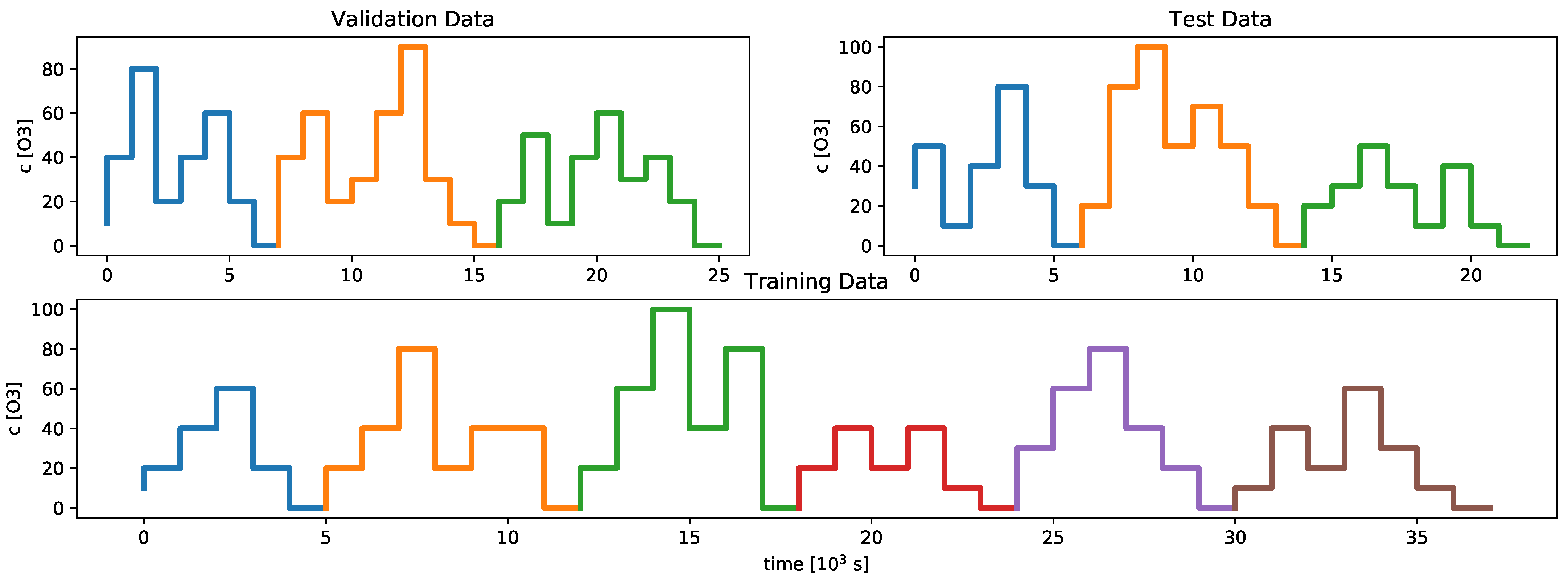
Throughout our studies, three different ozone concentration profiles were simulated for training, validation and testing. These concentration profiles are divided into differently shaped subprofiles. In order to create the dataset, several sequences of these subprofiles have been created and simulated. The different subprofiles for the training, validation and test dataset are shown in Figure 2. The reason for generating several permutations of these subprofiles is to prevent models from overfitting and to decrease drift-related effects due to slow recovery as well.

In terms of feature engineering, different types of input data have been used. The raw signals from three different simulated sensor materials with different functionalization and pulsed temperature modulation between two temperatures ($T_{low}$ = 65 °C, $T_{high}$ = 135 °C) have been preprocessed by removing the high-temperature signals and averaging the remaining signal over a certain time scale. Each data point represents 20 s of measurements. Furthermore, the three derivatives of the sensor signals have been calculated and used as an input. Additionally, so-called energy vectors have been calculated and used as an input as well [30,31]. These data points represent the energy between every combinatorial subset of two sensor signals. One sample of the energy vector $E_{ij}$ between the i-th and j-th sensor signal is defined by the following equation:

$$E_{ij}={\int }_{t_0}^{t_1}{s}_1\left(t\right)s_2\left(t\right)dt$$

(1)

Here, $s_1\left(t\right)$ and $s_2\left(t\right)$ describe the two sensor resistance signals. In our measurements, the energy vectors are calculated as a discrete sum over several measurement samples. As a feature, energy vectors can additionally stabilize the input data, since they take the history of the measurements, to some degree, into account. This information is especially useful for non-recurrent approaches, such as the MLP or the SVR algorithm.

Overall, the dataset, which was used for the robustness evaluation, contained 11,391 samples for the training set, 3444 samples for the validation set and 3444 samples for the test set. Examples for the data that were used in the different studies are depicted in the supplementary material.

2.1.3. Performance Metrics

Another substantial point in the evaluation process of machine learning models is the choice of metrics to compare the performance of a regression algorithm. These metrics usually map different aspects of the algorithm performance on a scalar value and are more sensitive to certain aspects of the performance than to others. Therefore, we decided to calculate an array of different metrics in order to obtain a detailed picture of the machine learning model performance.

Two metrics that are very commonly used for such purposes are the mean absolute error (MAE) and the root mean square error (RMSE).

$$\mathrm{MAE}=\frac{1}{N}\sum _{i=1}^N|y_i-{\widehat{y}}_i|$$

(2)

$$\mathrm{RMSE}=\sqrt{\frac{1}{N}{\displaystyle \sum _{i=1}^N}{\left(y_i-{\widehat{y}}_i\right)}^2}$$

(3)

These metrics penalize deviations from the ground truth without additional weights. The RMSE metric, however, is more sensitive to larger deviations and therefore also to outliers.

Furthermore, the $R^2$ score, also known as the coefficient of determination, was used as a metric.

$$R^2=1-\frac{{\sum }_{i=0}^N{\left(y_i-{\widehat{y}}_i\right)}^2}{{\sum }_{i=0}^N{\left(y_i-\overline{y}\right)}^2}$$

(4)

As a fourth performance indicator, a relative error metric was used. Specifically, the mean absolute percentage error has been implemented.

$$\mathrm{MAPE}=\frac{100}{N}\sum _{i=0}^N\frac{|y_i-{\widehat{y}}_i|}{y_i}$$

(5)

Due to its definition, the MAPE metric places an emphasis on the errors in the low-concentration domain, since the denominator has a higher impact on the overall error value for small gas concentrations.

2.2. Shapley Value-Based Feature Ranking for Environmental Sensor Algorithms

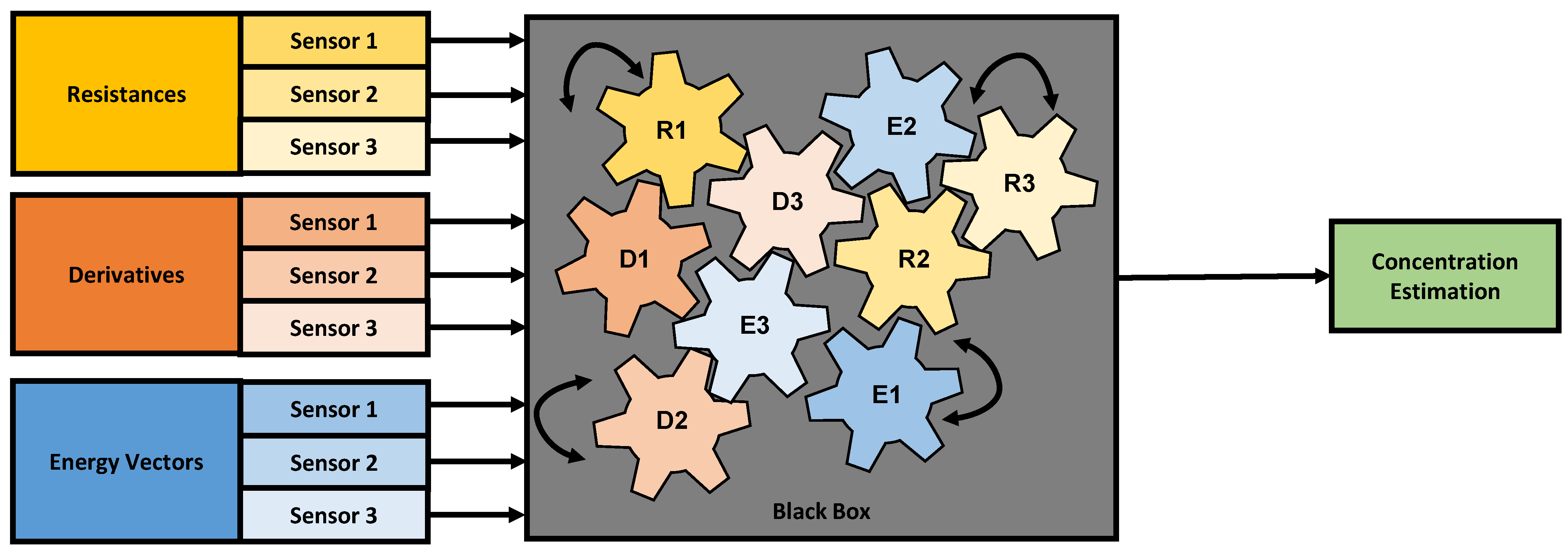
Machine learning models, especially neural networks, are capable of combining different types of features in a nonlinear manner to form a classification guess or a prediction. However, the inner reasoning inside of such algorithms is often not comprehensible for the user and the algorithm is perceived as a “black box” [32,33] (as illustrated in Figure 3), which makes technologies relying on such algorithms prone to undesired effects that cannot be determined in the algorithm production stage.

Therefore, explainability methods are necessary to be able to analyze the working principle of the algorithms. For environmental sensors, these considerations apply as well, especially when instabilities in the sensor behavior are likely to occur and are not covered in the training data set.

As far as algorithms for chemiresistive gas sensors are concerned, there have been only few studies trying to tackle the problem of missing explainability. We observe that feature ranking techniques are often used for choosing, enhancing or engineering features. Hayasaka et al. developed a graphene field-effect transistor sensor, which runs a feed-forward neural network architecture for the classification of different vapors. In their work, they used an ANOVA F-test to rank the different sensor features with regard to their importance. They concluded that the electron field-effect mobility was the feature providing the most important information [34]. A second method involving a statistical test for feature ranking was used by Leggieri et al., performing a ${\chi }^2$ statistical test on their electronic nose input features [35]. Liu et al. used a feature ranking method for filtering out redundancies in the sensor features [36]. Zhan et al. used a signal-to-noise ratio (SNR) method for feature selection for the classification of herbal medicines [37].

In this paper, we resort to a state-of-the-art method to derive the importance of different features on the prediction of gas sensor algorithms. The method that we used for our feature ranking investigations is called SHAP, which was developed by Lundberg et al. [38] and is derived from game theory. Differently from ANOVA, this technique attempts to interpret locally and on an algorithm level how each input feature of a machine learning model contributes to the algorithm’s prediction. In order to quantify the contribution of a feature to the overall prediction, SHAP values need to be calculated by combining features of LIME [39] and the general Shapley values [40]. In order to explain a complex model, SHAP aims to approximate the model locally for an input feature by a linear explanation model g, which describes a linear function with respect to the presence of different subsets of the M features summarized by a so-called coalition vector $z^{\prime }\in {\{0,1\}}^M$ [41]. The feature-specific weights of the linear explanation model ${\varphi }_j$ describe the impact of the j-th feature on the local prediction.

$$g\left(z^{\prime }\right)={\varphi }_0+\sum _{j=1}^M{\varphi }_j{z}_j^{\prime }$$

(6)

The calculation of the feature attributions ${\varphi }_i$ through SHAP for each prediction sample to explain the concrete prediction value is then used to visualize and quantify the importance of each individual feature of the algorithm.

2.3. Simulation of Different Sensor Instabilities

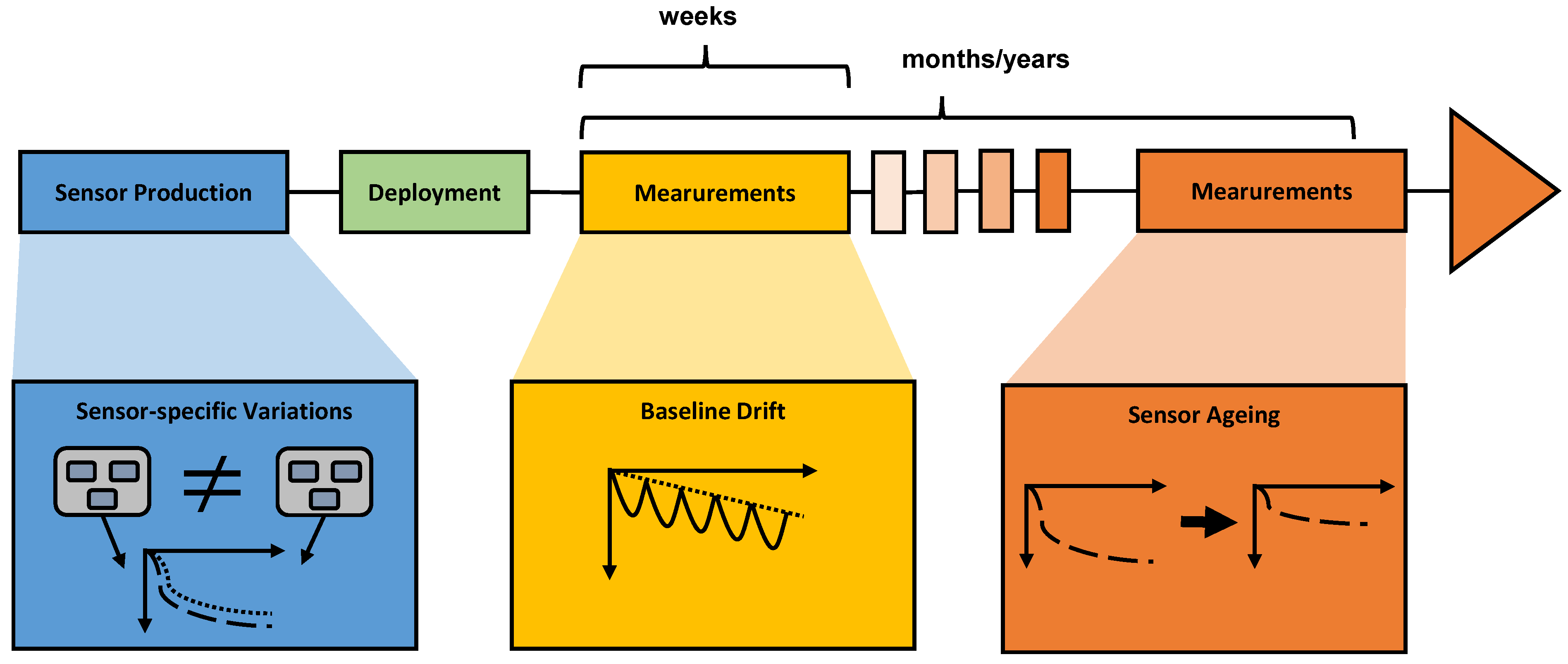
This section focuses on the different simulation techniques and objectives that are to be studied in terms of algorithm robustness. The section on device-specific variations focuses on effects that occur during sensor production and pre-treatment. The part on sensor drift emphasizes the impact of a medium-term effect on the sensor performance. Subsequently, long-term effects are described in the section on sensor ageing.

2.3.1. Sensor-to-Sensor Variations

Reproducibility is an important aspect in the fabrication of chemiresistive gas sensors. In the production process of such devices, it occurs that similarly processed sensors, even from the same batch, show slightly different physical characteristics in their measurement properties when measured in similar conditions [42]. This means that different sensor devices of the same type can show a different reaction, when they are exposed to the exact same concentration profile. In other terms, the sensors produce different signals for the same gas concentrations.

This represents a problem for the development of gas sensor algorithms. The machine learning models that are deployed on new sensor devices are trained on measurements recorded from a small batch of devices or even a single device. When deploying such an algorithm on a new device showing different measurement characteristics, the performance in terms of gas prediction might diminish.

The field in which methods to compensate for such effects are studied is called “Calibration Transfer”. Here, algorithms are investigated that map the signals obtained by slave devices (new sensors, which were not part of the measurement calibration process) to a master device. Different algorithmic techniques were studied by researchers in terms of their performance to achieve calibration transfer for different devices [43,44,45,46,47].

In terms of evaluating the impact of sensor-to-sensor variations on the prediction performance of chemiresistive gas sensors, few studies have been published. Bruins et al. investigated the changes in sensor data heterogeneity, if sensors show temperature shifts compared to each other. Throughout their studies, they conclude that strict temperature control is necessary for chemiresisitve sensor reproducibility and that temperature in general has a rather strong effect on the data heterogeneity compared to morphological variances [48].

In order to study the impact of such sensor-to-sensor variations, we performed different simulations. In the proposed study, we investigated the effect of different sensitivities on the sensor surface and their impact on the algorithm performance. One of the model parameters of our sensor simulation model [14] is the so-called splitting factor. It describes the ratio between sites associated with higher and lower energies on the sensor surface. This ratio can be either influenced by the concrete production process of the sensor material or by the pre-treatment of the material performed on the sensor before release. Variations in these processes ultimately alter the sensor sensitivity.

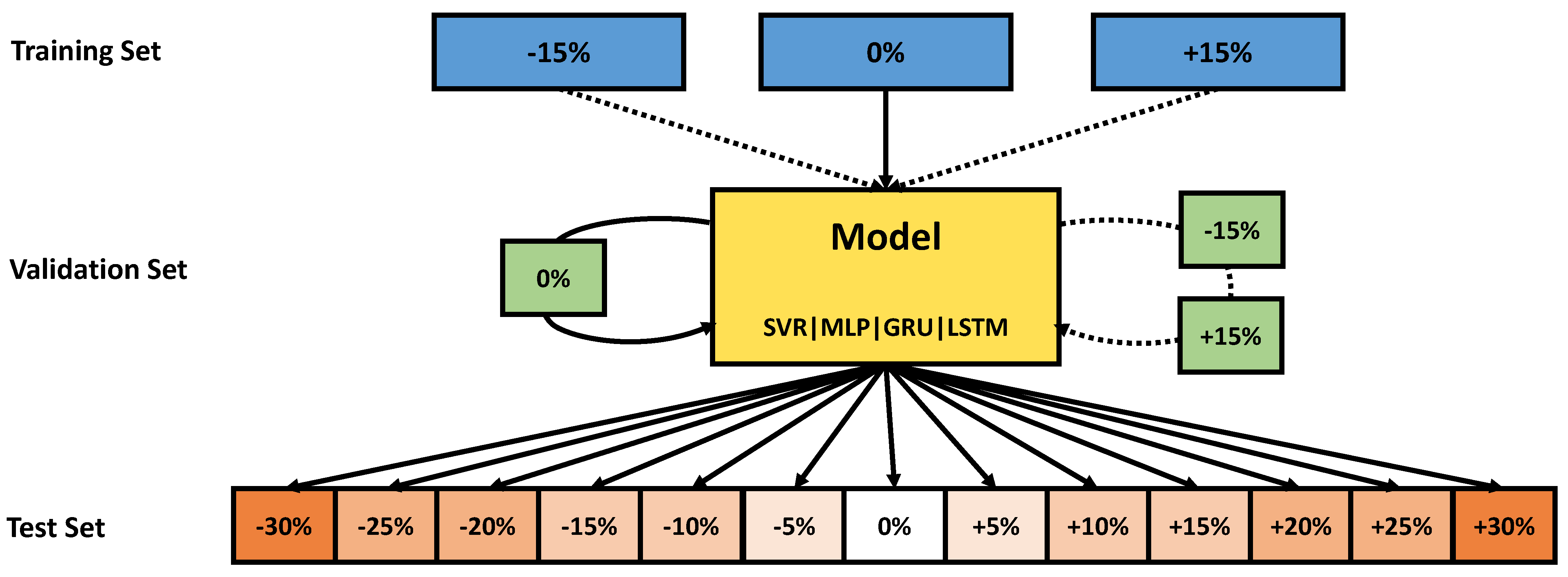
In our study, we were therefore altering the splitting factor in order to simulate the differences in production and pre-treatment and analyze them in terms of their algorithm performance impact. The test set concentration profile was hence simulated with deviations from the standard parameter between −30% and $+30\%$ in $5\%$ steps.

In a second step, we investigated whether additional variation in the training data can increase the robustness of the regression models. To this end, we augmented the training set with additional sensor data simulated with parameter deviations of $-15\%$ and $+15\%$. The model was then tested on the test sets of the previous experiment. An overview of the different data configurations of the experiments is shown in Figure 4.

2.3.2. Sensor Drift

In our second study, we analyze the impact of different additive and multiplicative drift states on the sensor algorithm performance. In the literature, Llobet et al. studied the impact of drift and other effects on the sensor measurement features, resorting to a PCA plot for different gas mixtures. The data were obtained by a simulation tool based on PSpice, which was presented in their paper [49]. Brahim-Belhouari et al. evaluated the classification performance of a tin-oxide sensor using a Gaussian mixture model with respect to the additive sensor drift behavior. They found a strong decay in sensor accuracy due to drift and could partially compensate for the accuracy loss by retraining the model, which enhanced the robustness of the algorithm [50]. In another work, Vergara et al. proposed a classifier ensemble technique for drift compensation. In their work, they analyzed the classification performance decay for different classifiers over the course of 36 months without drift compensation. They found that the application of ensemble classifiers for drift compensation can significantly reduce the accuracy decay caused by sensor drift [51].

To carry out our analysis, we altered the original test data signals by applying additive and multiplicative drift of different levels onto the signal. Furthermore, the simulation of the original training, validation and test set was different compared to the other studies. For the dataset of the drift study, a long concentration pulse has been simulated, followed by a short period of time without a gas present, before the actual concentration profiles were simulated. At the beginning of the actual concentration profile, a recalibration of the sensor signals has been performed. This is done in order to reduce the initial drift of the sensor in the dataset and hence obtain a more stable sensor signal, so that the impact of different drift levels can be analyzed without interference of other drift effects.

In order to create a test set with different levels of drift, a definition of the levels for the additive drift is necessary in order to quantify the amount of drift relative to the sensor signal. Since the simulation output signals describe already the relative resistance calibrated to zero, a measure has to be defined, which is relative to the signal itself, in order to measure the magnitude of the additive drift. Therefore, we take the difference between the minimum and the maximum resistance of the training dataset for each sensor as the span of values used for training and apply ratios of this value span to the baseline drift.

$${\mathbf{d}}_{drift}=\underset{i}{min}\left\{{\mathbf{R}}_{i,train}\right\}-\underset{i}{max}\left\{{\mathbf{R}}_{i,train}\right\}$$

(7)

Here, $\mathbf{R}$ describes a vector of the three sensor signals and ${\mathbf{d}}_{drift}$ a vector of three value spans of the signals.

For the multiplicative drift, the signals, which were already calibrated to a baseline around zero, were multiplied with different multiplicative drift values. This influences the value span of the different test measurements and hence produces a multiplicative drift of the sensor signals.

The regression models were trained on the undrifted training set and validation set and then evaluated on the test sets with the different levels of additive and multiplicative drift.

2.3.3. Sensor Ageing

The ageing process of a chemirestive sensor over its lifetime can lead to different effects. In our third study, the ageing process characterized by sensitivity loss is simulated and analyzed. In the literature, Fernandez et al. investigated different sensor damage types and quantified their impact in terms of performance degradation with the mean Fisher score. They concluded that sensor ageing had a significant negative impact on the sensor performance, also in comparison to the other damage types [16]. In another investigation, Skariah et al. studied the impact of ageing of a Mg-doped tin-oxide gas sensor. They could measure a significant decay in the sensor’s response to the target gas of up to $50\%$ in 96 months [52].

In order to quantify the performance loss of the algorithms due to sensor ageing for our algorithm setup, the test profile was simulated multiple times, with different adsorption sites on the modeled sensor surface continuously covered. Throughout the simulation, these adsorption sites were treated as adsorbed and no new molecules were able to adsorb onto these sites, resulting in lower sensitivity. The simulated sensor signal was recalibrated in the beginning of the simulation, assuming that the simulation process starts after cleaning the still responsive parts of the sensor surface.

The fraction of adsorption sites that were put on hold describes the ageing state in the simulation procedure. The fraction was iterated between 0 and 0.9 in steps of 0.1, where 0.9 represents a sensor, where $90\%$ of the originally available adsorption sites are continuously adsorbed and non-responsive to new gas molecules. The regression models were trained on the respective profiles without sensor ageing and then tested on the test profile simulated with the different ageing states.

3. Results and Discussion

In this part, the different results of the previously described experiments are presented and discussed. First, the regression performance and explainability of the model without instability effects is shown. Subsequently, the different robustness studies are illustrated.

3.1. Regression Performance and Model Explainability

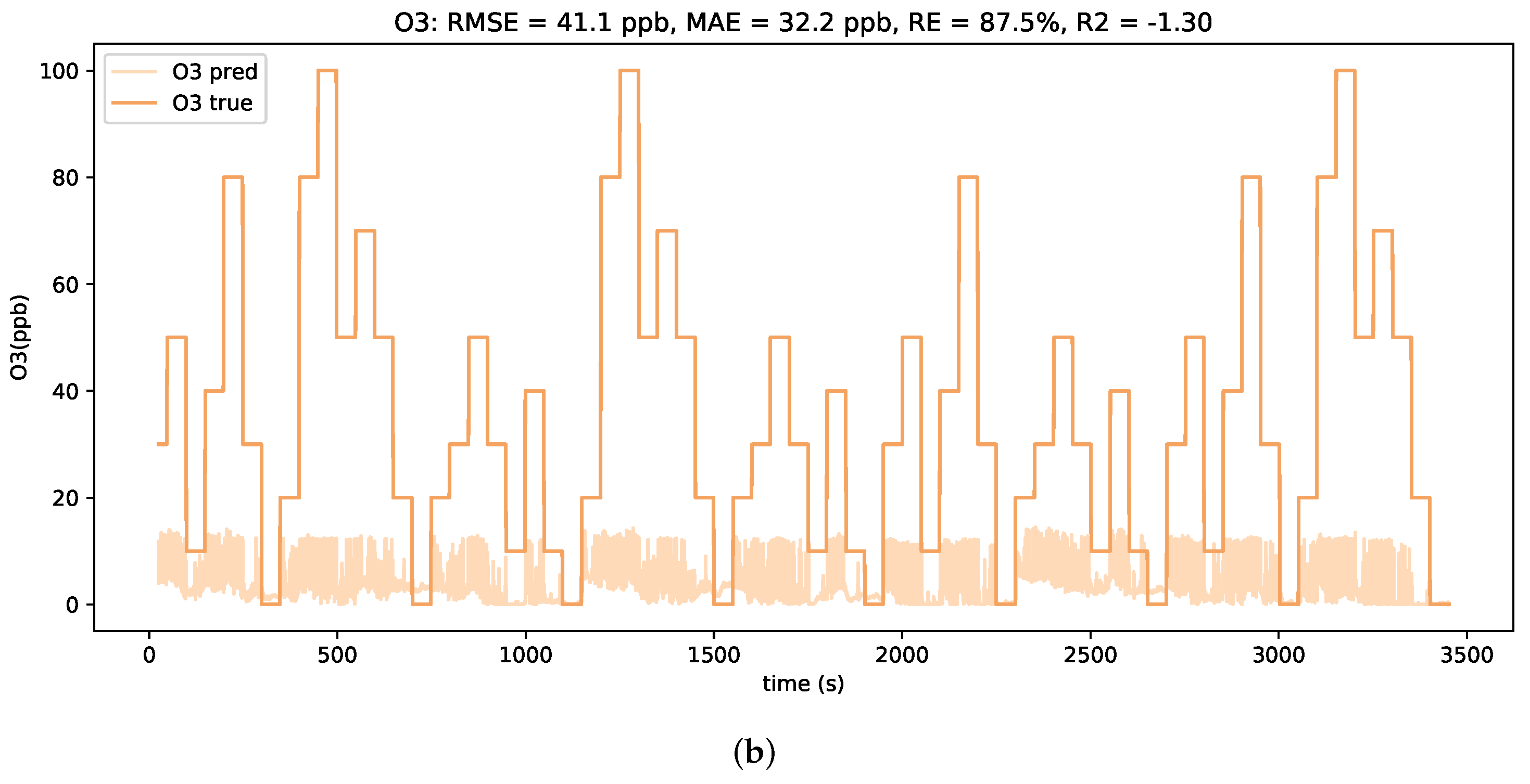
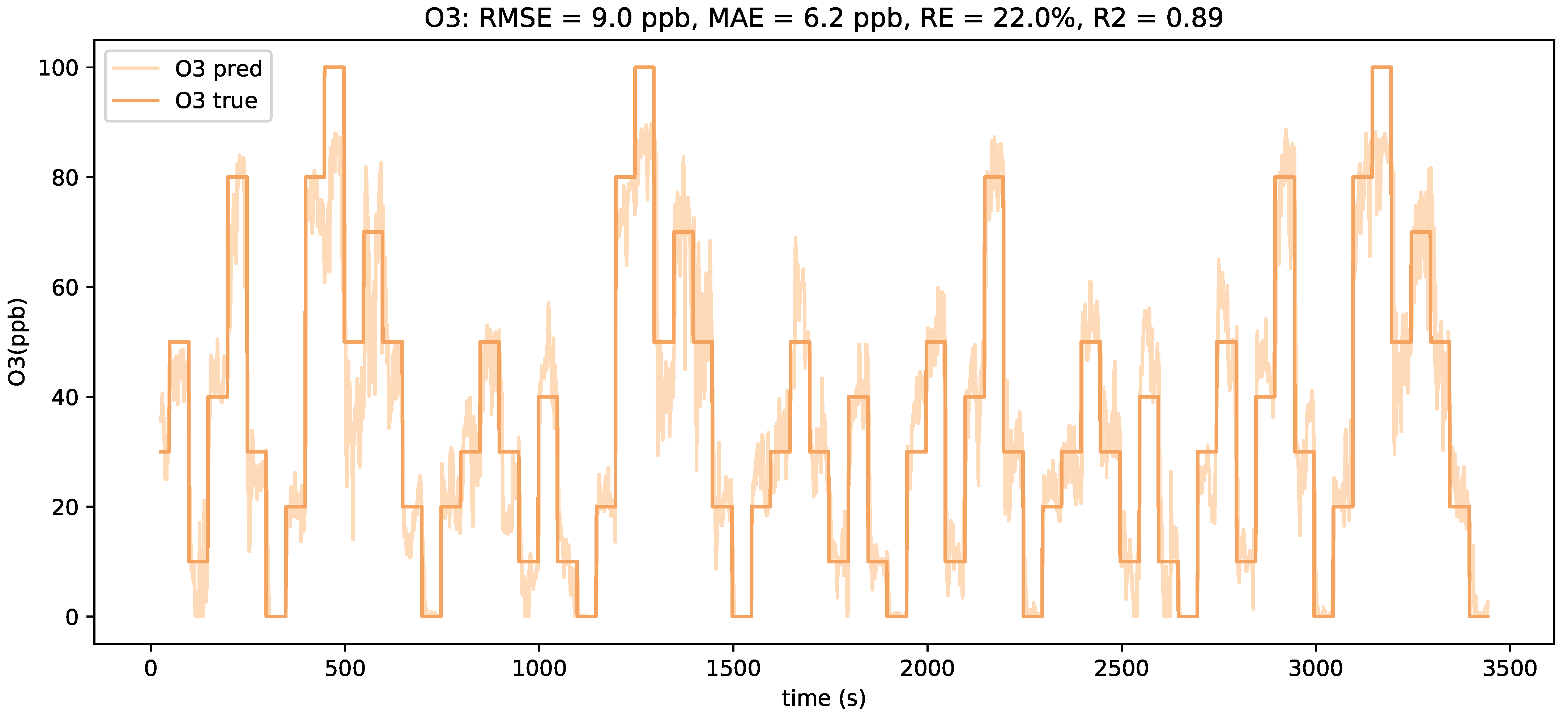
The different regression models were trained by making use of the training and validation set. Figure 5 shows the predictions of the LSTM model compared to the ground truth of the ozone concentration. Despite the predictions showing some noisy behavior, the overall concentration estimates are in good alignment with the real concentrations.

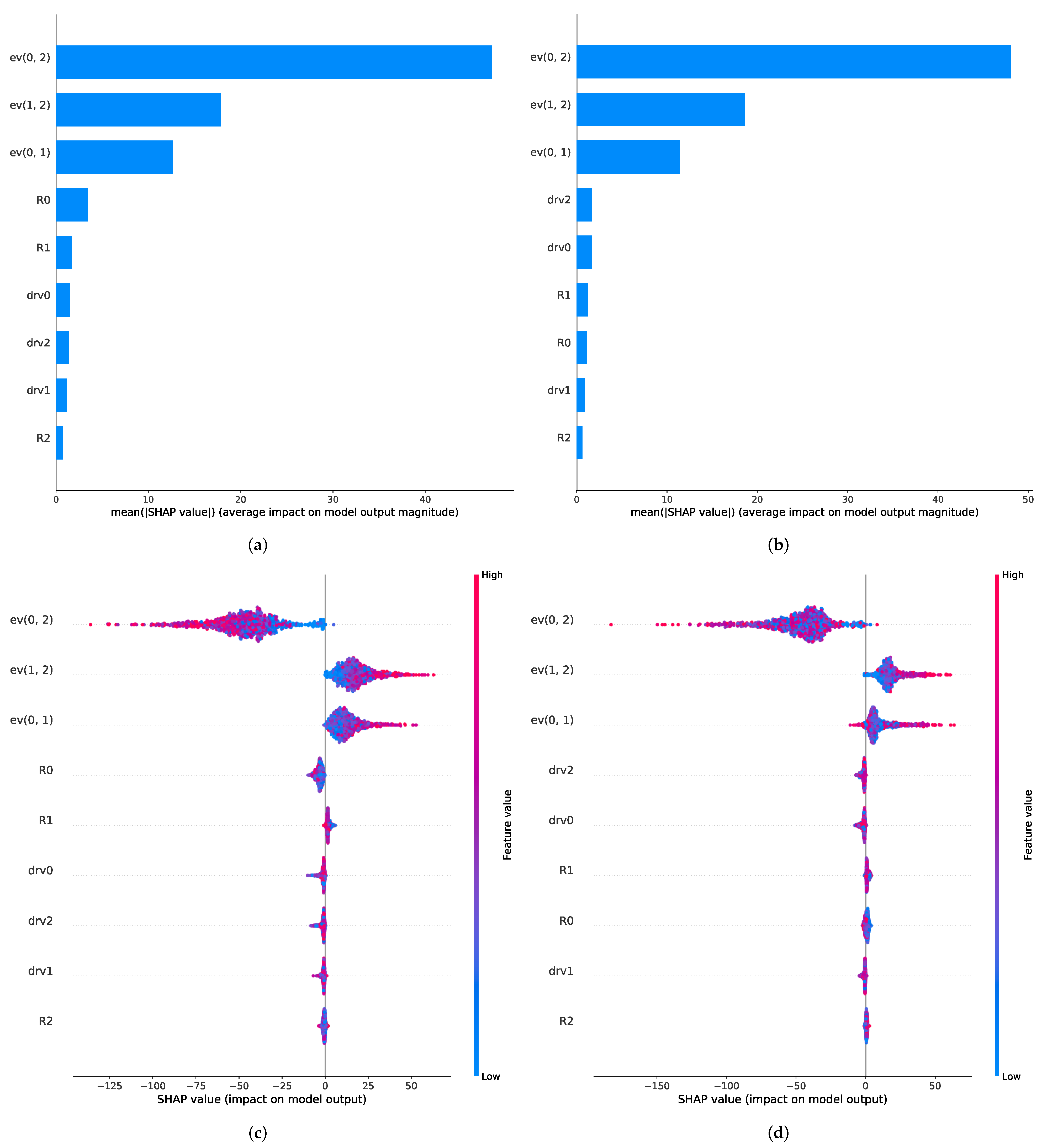
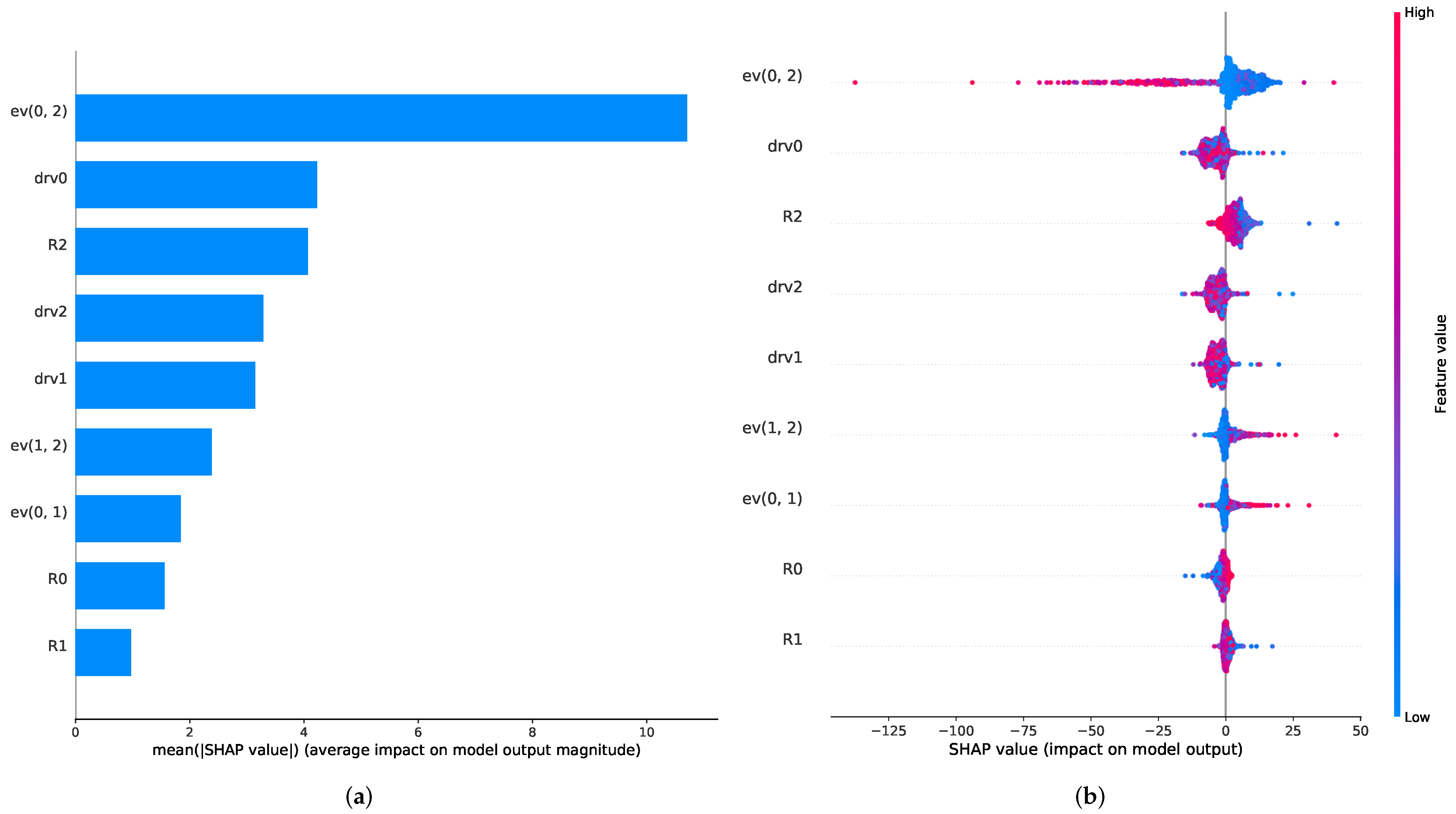
The results of the Shapley-value-based feature importance analysis are shown in Figure 6. It can be observed that for both RNN approaches, the energy vector features seem to have the main share in the gas estimation procedure as all three of the energy vectors rank the highest for the GRU and the LSTM model. After this, the relative resistance of the first and second sensor (R0 and R1, for the LSTM) and the derivatives of the first and third sensor (drv0 and drv2, for the GRU) play a minor part in the prediction process.

A more detailed analysis of the model output impact depicted in Figure 6c,d shows that the different energy vectors seem to influence the regression outcome in opposite ways. The energy vector of the first and third signal (ev(0, 2)) has a negative impact on the concentration prediction, whereas the other two energy vectors have a positive impact. This suggests that ev(0, 2) is used for the baseline drift compensation of the absolute sensor features, since it lowers the prediction, especially for high energy feature values. It has to be added that a negative impact of the energy vector for high values is needed for drift compensation, since a downwards drift in the resistance signal leads to an upwards drift in the energy vector signal. The other two energy vectors tend to increase the concentration prediction value for high energy vector values, which suggests that they recognize relative changes in the drifting sensor signals.

We note that the focus on one feature group is an important characteristic to monitor during sensor algorithm development. A non-diversification of features can have an impact on the performance of the algorithms in the presence of additional effects, such as sensor instabilities, which might be specifically affecting the corresponding feature group. Finally, we observe that, for each new setup or change to the sensor implementation, a similar analysis should be repeated since the value of different features and hence the observed dependencies are highly dependent on the specific technology characteristics.

3.2. Sensor-to-Sensor Variations

The section on sensor-to-sensor variations is structured into two subsections. In Section 1, the study on the impact of sensitivity changes is shown. Subsequently, the change in sensor performance by augmenting the training dataset with data containing such variations is analyzed.

3.2.1. Sensitivity Variations

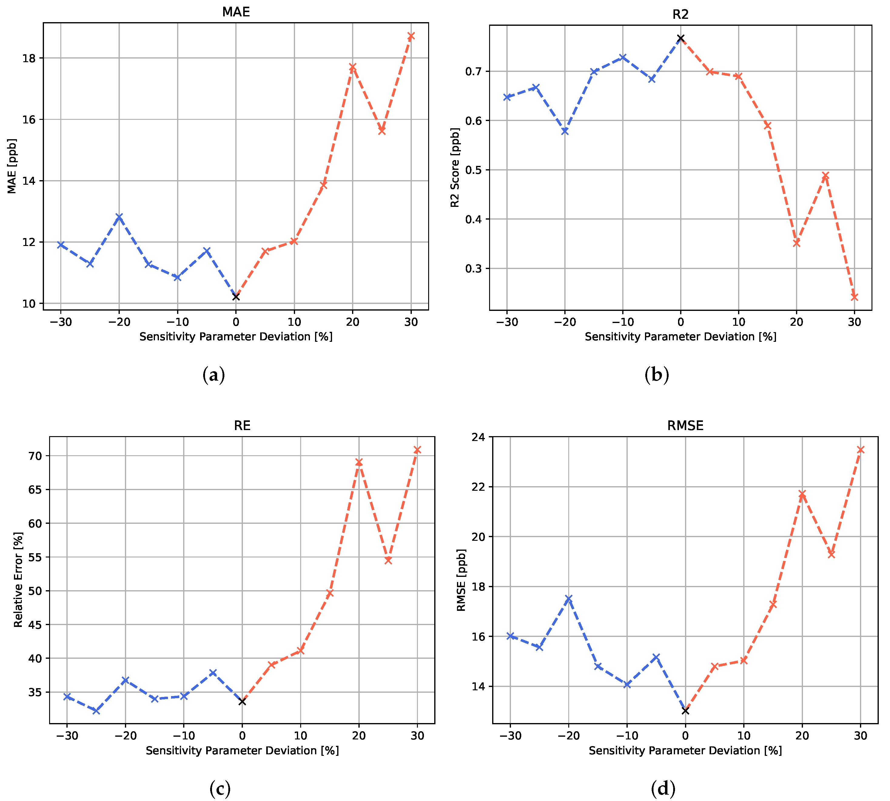
For the study on sensitivity variation, machine learning models, which were trained and validated on the standard sensitivity parameter, have been tested on the same test concentration profile simulated with a set of different sensitivity variations. The results are shown in both Figure 7 for the MLP variation and

Table 1. Comparison of the mean absolute error for different variations in the sensitivity parameter with respect to the regression algorithm.

Alg.	−30%	−25%	−20%	−15%	−10%	−5%	0%	+5%	+10%	+15%	+20%	+25%	+30%
SVR	12.1	11.55	12.98	11.26	11.07	11.53	10.59	11.9	12.11	12.84	16.64	14.74	17.37
MLP	11.9	11.29	12.82	11.27	10.85	11.71	10.21	11.7	12.03	13.85	17.72	15.61	18.73
GRU	6.22	6.41	7.48	6.53	6.28	6.34	6.43	6.06	6.17	6.09	7.32	6.82	7.01
LSTM	6.67	6.66	7.02	6.67	6.18	6.55	6.15	6.15	6.29	6.16	7.45	6.61	6.99

for all algorithms.

In Figure 7, it can be seen that, for the MLP algorithm, the variation in the sensitivity parameter has a noticeable effect on the algorithm’s prediction performance. Moreover, when analyzing the different error metrics, the data suggest that the positive and negative deviations from the original sensitivity parameter lead to a performance degradation. A negative deviation seems to lower the prediction accuracy in the higher concentration range, since the relative error appears to be rather stable, while the RMSE shows an increase for negative parameter deviations. The positive sensitivity parameter deviations are shown to have a strong impact on all error metrics. In the simulation, a positive deviation from the sensitivity parameter is connected to a stronger drift behavior. This signal behavior seems to have a stronger effect on the model performance than the enhanced relative sensitivity associated with the negative sensitivity parameter variations.

For the recurrent neural networks, the negative deviations of the temperature parameters seem to have statistically no noticeable negative effect on the prediction performance. For both recurrent architectures, a small increase in the MAE can be seen for positive parameter changes. A reason for this difference towards the other algorithms might be that the focus of the recurrent algorithms on the historical development of the feature values might make them less prone to the lower drift and higher sensitivity characteristics of the negative parameter deviations.

3.2.2. Robustness for Augmented Training Profiles

In an additional experiment, we took the algorithm robustness analysis one step further by investigating whether a more diverse dataset would be capable of increasing the stability of the algorithm to the sensor-to-sensor deviations. By training with both the original training data and the same data with $-15\%$ and $+15\%$ sensitivity parameter deviation, we performed the same analysis as in the previous section. 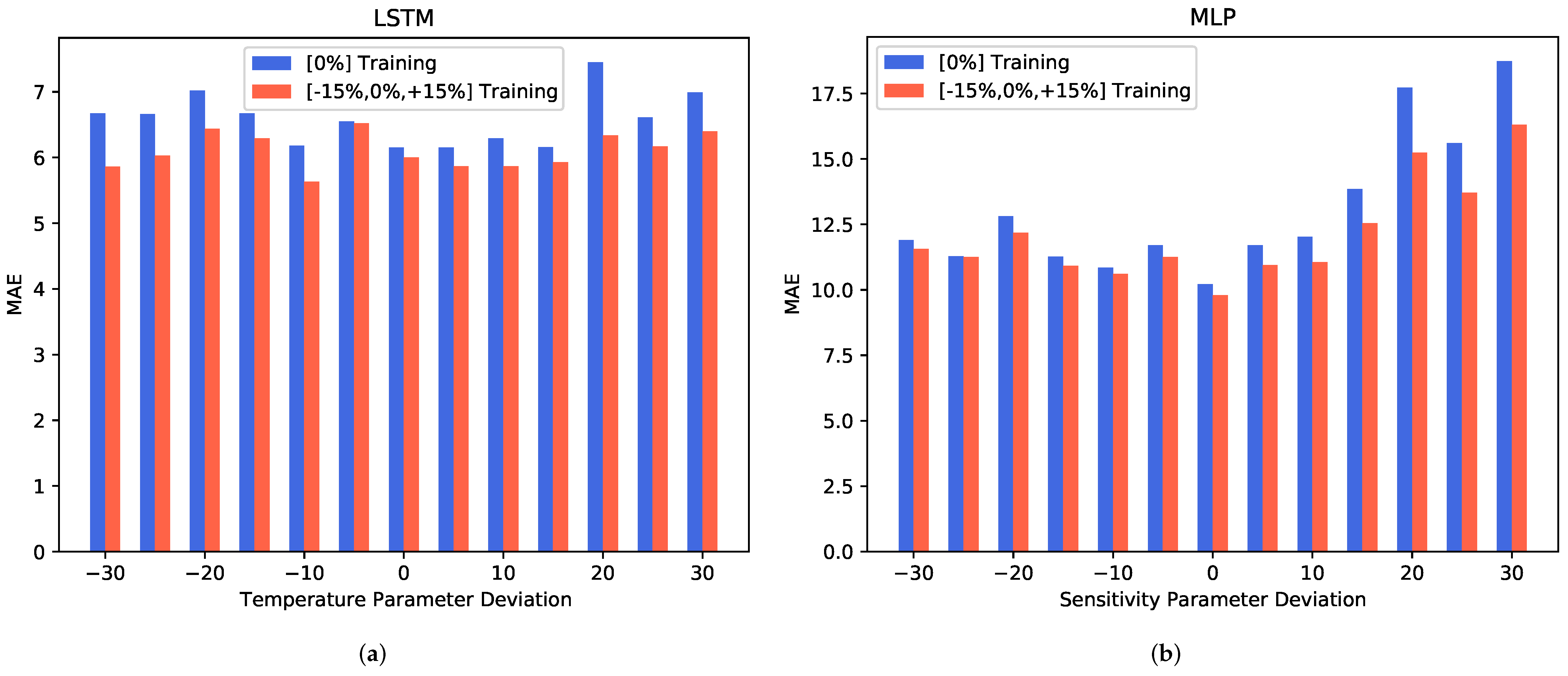A comparison between the original results and the results from this more diverse training data case is shown in Figure 8.

It can be observed that training with a diverse dataset has a positive impact on the prediction performance. For the LSTM model shown in Figure 8a, a decrease in the MAE can be seen on both extremes of the parameter deviation scale. The MLP model, which is depicted in Figure 8b, shows a much stronger increase in the prediction performance for the positive sensitivity parameter deviation levels.

Overall, our data show that a diversification of the training dataset can improve, to some extent, the prediction performance in the presence of sensor-to-sensor variations linked to the sensitivity. Depending on the algorithm, the improvement might be limited to certain types of sensitivity changes.

3.3. Drift Effects

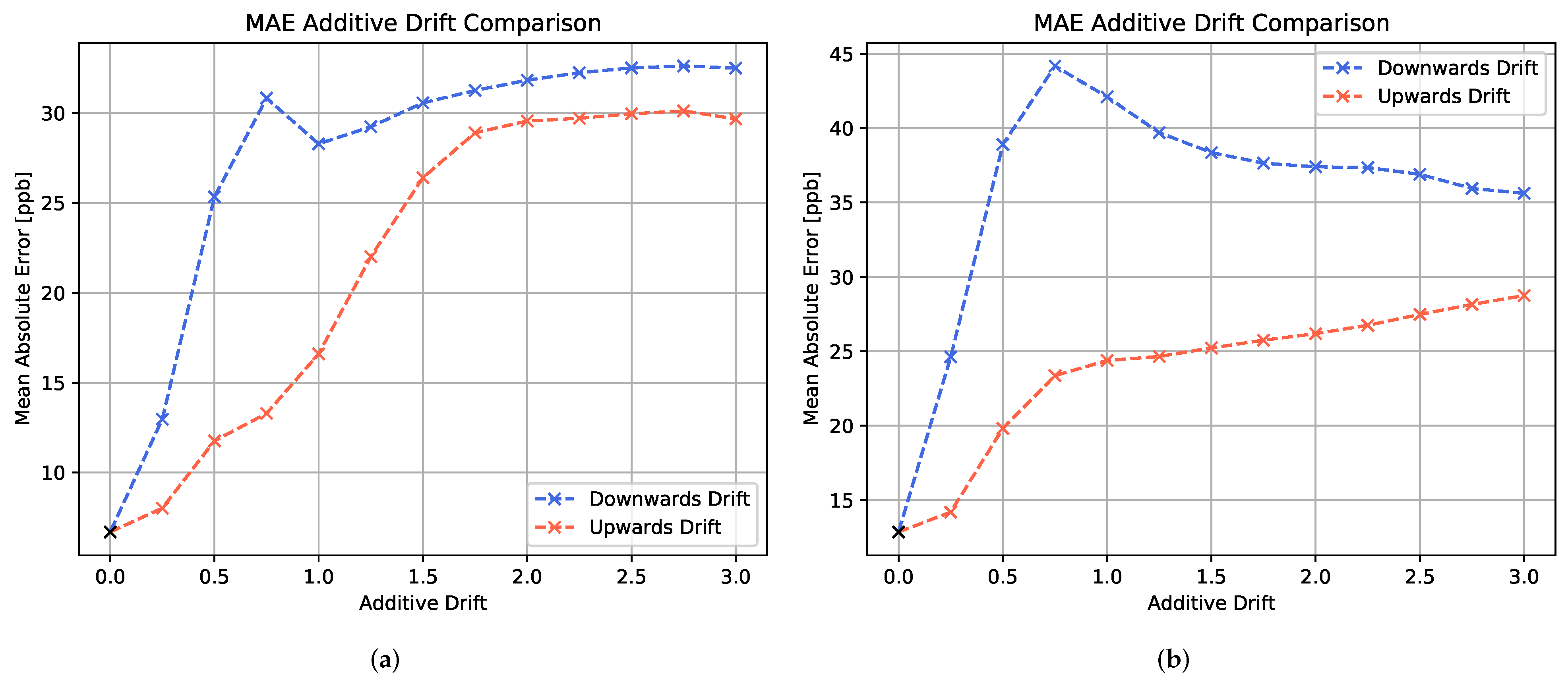
In this section, we wish to review the experiments on additive and multiplicative drift and their influence on the gas prediction performance. Figure 9 shows the mean absolute errors for (a) the LSTM model and (b) the MLP model with respect to different levels of additive drift. For both models, a strong decay in prediction performance is observed in the presence of additive drift. The downwards drift leads to a considerably faster increase in MAE than the upwards drift.

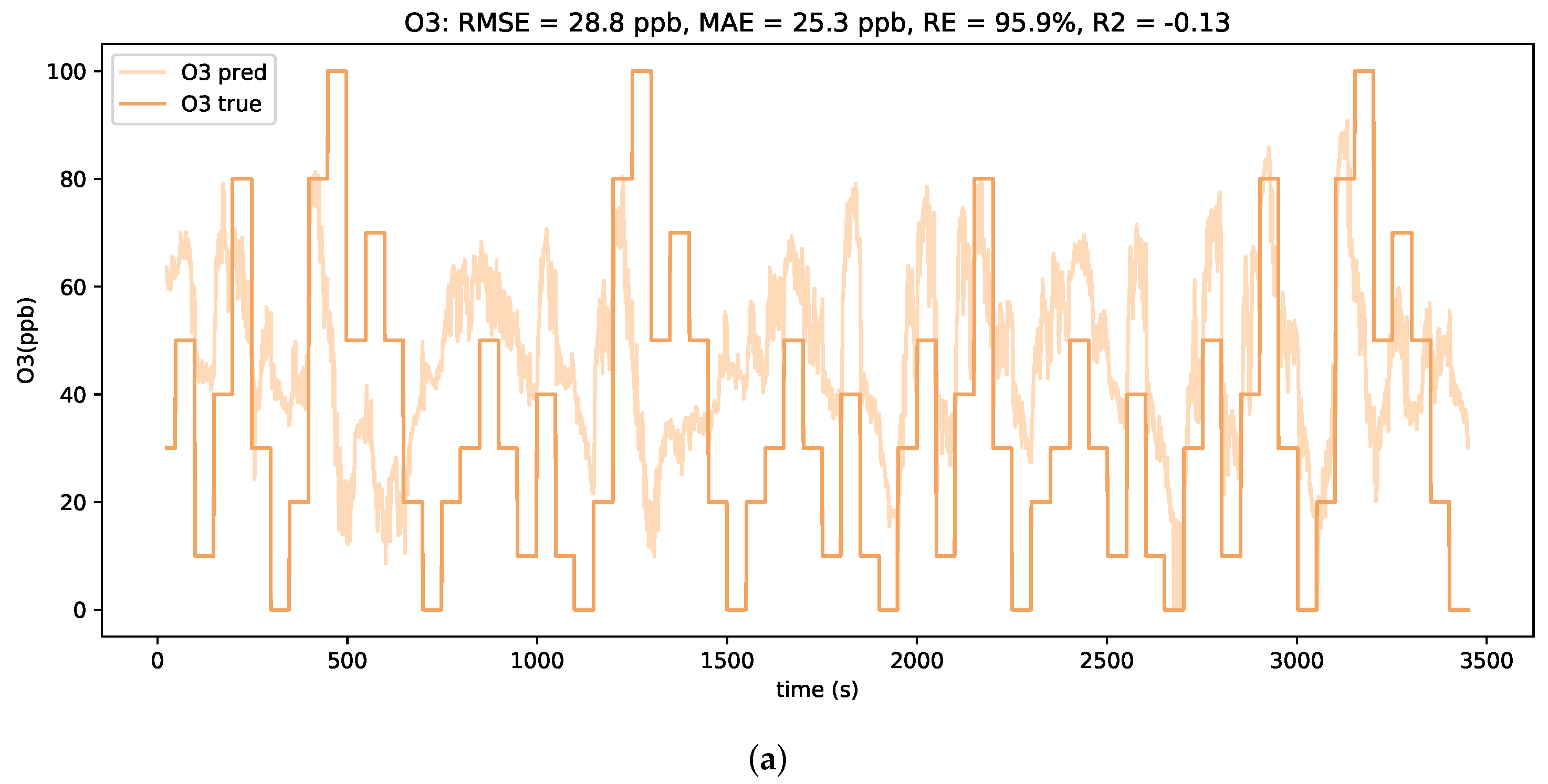
It is noted that a peak occurs in the MAE curve at around 75% of additive downwards drift. When comparing the concentration estimation plots for test profiles with lower levels and higher levels of downwards drift, as depicted in Figure 10, clear differences in the prediction behavior are observed. For smaller downwards shifts of the signals, the LSTM model tends to severely overestimate the low concentrations. However, a general alignment with relative concentration changes is still visible. In contrast, for larger downwards shifts of the signals, the LSTM model only predicts in a considerably small concentration range. It is assumed that such strong shifts in absolute signal values are beyond the scope of the trained neural network model and hence lead to unfeasible predictions.

The effect that the upwards drift appears to have a smaller, but still noticeable, impact on the sensing performance might be explained by analyzing the feature importance, as illustrated in Figure 11. This shows that, similarly to the previous model for the sensitivity analysis, the main contributor to the concentration prediction is the energy vector between the first and the third sensor. Additionally, the derivatives are observed to play a stronger role in the prediction as well as the resistance value of the third sensor. During the upwards drift experiment, the energy vectors change less in their absolute values compared to the downwards drift experiment. This means that the state of overestimation observed at low levels of downwards drift is only reached at moderate levels of upwards drift. This might explain the slower decay behavior for the upwards drift experiment.

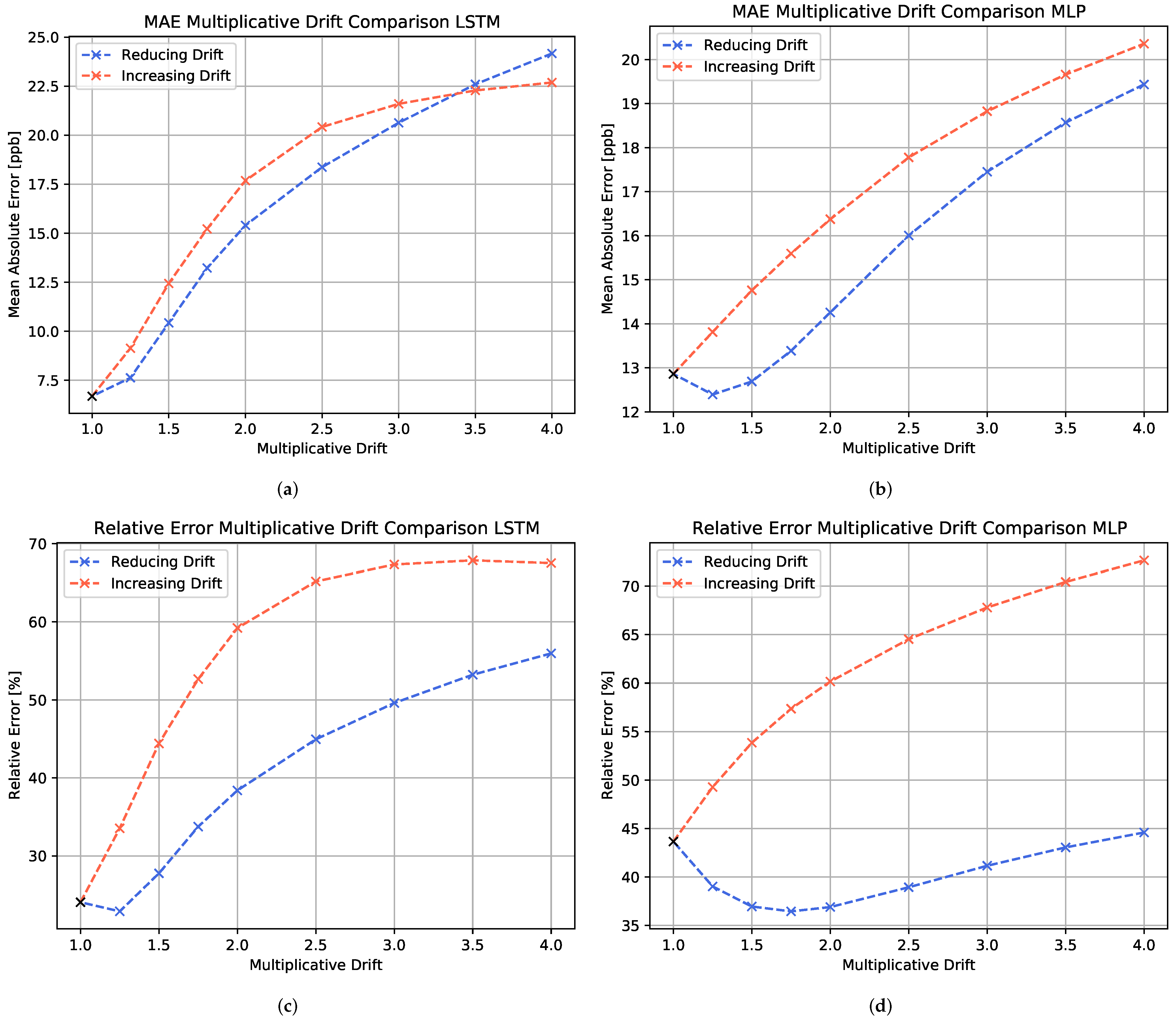
The evaluation of the performance loss due to multiplicative drift is shown in Figure 12. It is observed that the performance decay of the two different multiplicative drift directions is dependent on the evaluation metric. Overall, for both the LSTM model and the MLP model, the increasing drift seems to have a stronger impact on the model performance than the reducing drift. Only for high levels of multiplicative drift, the MAE of the reducing drift surpasses the increasing drift error. This means that the concentration overestimation due to increasing drift seems to worsen the prediction accuracy more severely than a slight underestimation.

For the MLP, the relative error shows even better performance values at moderate reducing drift values than the non-drifting case, whereas the MAE shows an upwards trend at these drift levels. This is due to a concentration overestimation of the MLP with respect to lower concentrations observed for the non-drifting test set. In this case, the reducing drift enhances the prediction accuracy for the lower concentration domains, while it leads to an underestimation of the higher concentration regions at advanced drift levels.

3.4. Sensor Ageing

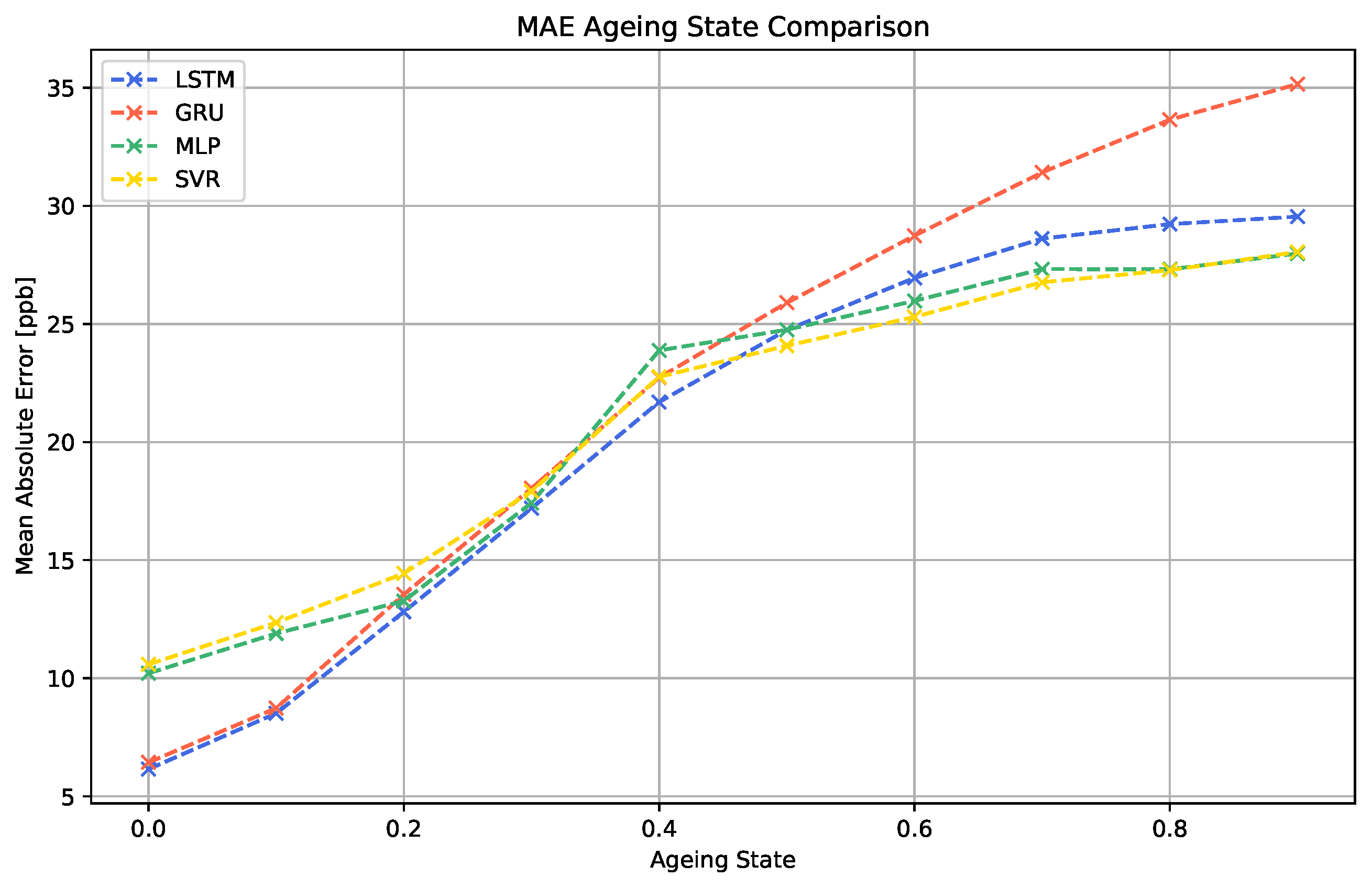
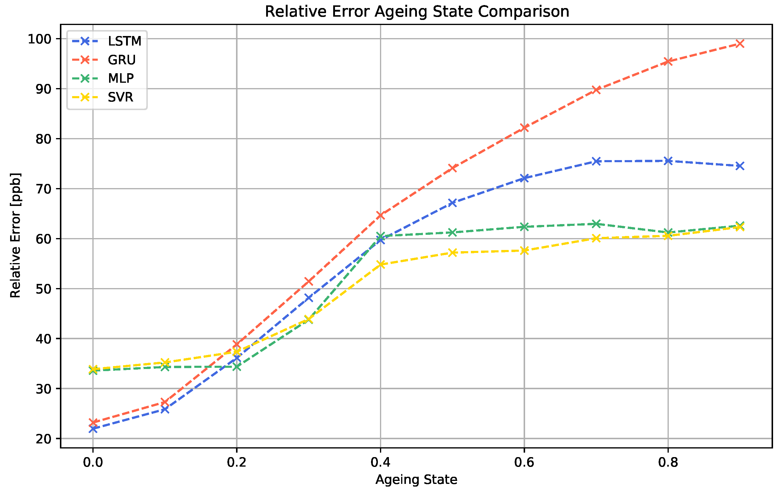
In a final study, the impact of sensor ageing on the performance of the different machine learning algorithms was investigated. The results of the simulated scenario are shown in Figure 13 and Figure 14.

The data show that the continuous ageing process clearly decreases the performance of all machine learning models. For all cases, the performance decay process starts quickly at 0.1. For the LSTM, MLP and SVR algorithms, the increase in the MAE becomes slower and finally saturates for higher ageing values above 0.6. The GRU algorithm does not show this saturation behavior.

Furthermore, it is noticeable that the two best-performing models for the sensor data without ageing effects, LSTM and GRU, generate considerably worse results for sensor signals showing advanced levels of sensor ageing than the MLP and SVR models. Since this effect is visible to both RNN models, this indicates that this property is linked to the recurrent nature of the models.

Our experiments show that, in terms of long-term stability, also models performing moderately under normal circumstances can show higher robustness to certain instabilities. In contrast, the more complex RNN approaches, even though better adaptable to the regression task, might need additional ageing compensation techniques in order to increase their robustness.

4. Conclusions

In this work, we developed and presented a scheme for characterizing and testing various machine learning algorithms on smart chemiresistive gas sensor devices in the presence of different instabilities by using a validated sensor model.

It was shown that explainable AI methods, such as SHAP [38], provide significant insights into the roles of the various features in the prediction process. We have also seen that sensor-to-sensor variations due to sensitivity differences can lead to a strong decay in prediction performance, which can only partially be compensated by training set diversification.

Additive and multiplicative drift can lead to a strong decay in the prediction performance. The impact of drift on machine learning models varies among the drift types and the drift direction. Moreover, it was found that the sensitivity loss due to sensor ageing leads to significant performance decays, even having a stronger effect on more complex algorithm architectures.

Overall, our work substantiates the need for a thorough characterization of algorithm robustness when dealing with low-cost chemiresitive gas sensors. Even though models can never capture every detail of a sensor’s complexity, they provide a meaningful and necessary tool for algorithm characterization. In future investigations, the evaluation of sensor robustness shall be further extended to additional effects such as sensor poisoning or environmental changes [53,54].