Conservative Finite Volume Schemes for Multidimensional Fragmentation Problems

Abstract

In this article, a new numerical scheme for the solution of the multidimensional fragmentation problem is presented. It is the first that uses the conservative form of the multidimensional problem. The idea to apply the finite volume scheme for solving one-dimensional linear fragmentation problems is extended over a generalized multidimensional setup. The derivation is given in detail for two-dimensional and three-dimensional problems; an outline for the extension to higher dimensions is also presented. Additionally, the existing one-dimensional finite volume scheme for solving conservative one-dimensional multi-fragmentation equation is extended to solve multidimensional problems. The accuracy and efficiency of both proposed schemes is analyzed for several test problems.

1. Introduction

Fragmentation, breakage or attrition, describe processes in which a single object is separated into at least two new objects. The reasons for breakage can be manifold but are often linked to some kind of stress exerted on the object, for instance thermal stress from heating and rapid cooling (or vice versa and cyclically)—a natural process specifically observed in deserts, leading to disintegration of rocks; or mechanical stress, applied for millenia in the process of grain milling. Nowadays, fragmentation plays a key role in several industrial sectors like mineral processing (e.g., comminution of ores [1,2,3,4]), reaction engineering (e.g., break-up of bubbles in reacting bubble columns for separation processes [5,6,7,8] or steel-casting [9]) or pharmaceutical industries (e.g., milling of active pharmaceutical ingredients to increase their solubility and uptake capacity in the human or animal body [10,11,12]).

Many objects, e.g., particles, bubbles or even rain drops, consist of different components resulting in their anisotropic structure. The probability of fragmentation upon stress therefore depends on the distribution of the components within the objects, i.e., each component adds an independent dimension to the fragmentation problem. In an attempt to describe these complex processes and make them accessible for model- and knowledge-based process design, optimization and control, multidimensional fragmentation equations have been proposed and used in different fields of application, see, for instance, the works [13,14,15,16,17].

Theoretical aspects on the existence of scaling solutions and their behavior at the onset of “shattering” transition have been discussed for instance in the works of [18,19,20,21]. Fragmentation models are particularly challenging as they consist of partial-integro differential equations as will be shown in the following. Analytical results are scarce and often of very limited practical relevance, strongly motivating the development of numerical methods for approximation of the solution to (multidimensional) fragmentation problems.

As a prototype, consider the conservative formulation of the multiple fragmentation equation given by [22,23]: The initial value problem for $t\ge 0$ is formulated as

$$\begin{array}{cc}\hfill \frac{\partial g(t,x)}{\partial t}& =\frac{\partial \mathcal{H}\left(t,x\right)}{\partial x},\mathrm{where}x\in {\mathbb{R}}^{+}:=(0,\infty ),\hfill \end{array}$$

(1)

with the initial condition

$$\begin{array}{cc}\hfill g(x,0)& {\displaystyle =g_0\left(x\right)\left(\ge 0\right),\mathrm{for}x\in {\mathbb{R}}^{+}.}\hfill \end{array}$$

(2)

The flux function $\mathcal{H}\left(t,x\right)$ is defined by

$$\begin{array}{c}\hfill \mathcal{H}\left(t,x\right):={\int }_x^{\infty }{\int }_0^x\frac{u}{v}b(u,v)S\left(v\right)g(t,v)\mathrm{d}u\mathrm{d}v,x\in {\mathbb{R}}^{+}.\end{array}$$

(3)

In Equation (1), the internal variables x and t denote the particle property and the time component, respectively. On the left hand side, the function $g(t,x)$ is defined by $g(t,x):=xf(t,x)$, where $f(t,x)$ denotes the distribution of particle volume x in a system at time t. The rate of selection of an x-volume cluster to undergo breakage is denoted by $S\left(x\right)$, and the distribution of daughter particles y due to the breakage of large particle x is denoted by $b(y,x)$. The breakage function $b(y,x)$ satisfies the following relations:

$$\begin{array}{c}\hfill {\int }_0^{\infty }b(y,x)\mathrm{d}y=\nu \left(x\right),\mathrm{and}{\int }_0^{x}yb(y,x)\mathrm{d}y=x.\end{array}$$

(4)

The first relation defines that $\nu \left(x\right)$ number of fragments are produced during the breakup of a large x-cluster, and the second relation defines that the total volume of the daughter y-clusters is exactly the same as the volume of the mother x-cluster. Note that the formulation (1) is well-known in the literature as the volume conservative form. Integration of Equation (1) over the volume variable x from 0 to ∞, with the help of relation (4), yields

$$\begin{array}{c}\hfill \frac{\mathrm{d}}{\mathrm{d}t}{\int }_0^{\infty }g(t,x)\mathrm{d}x=0.\end{array}$$

(5)

It should be noted that Equation (1) is a first-order hyperbolic, initial value partial differential equation. In this regard, the representation (1) gathered importance because the divergent nature allows the model to obey the volume conservation laws. The coefficient S belongs to $L_{loc}^{\infty }\left([0,\infty )\right)$ and $g_0,b\in L^1\left((0,\infty )\right)\cap L^1\left((0,\infty ),x\mathrm{d}x\right)$. Here and below, the notation $L^1({\mathbb{R}}^{+},x\mathrm{d}x)$ stands for the space of the Lebesgue measurable real-valued functions on ${\mathbb{R}}^{+}$ which are integrable with respect to the measure $x\mathrm{d}x$.

In most of the previous studies it is assumed that a single parameter, which is usually volume, mass or size of the particle, is sufficient to describe the particle property (readers can refer to [24] for further details). However, a single parameter is not always sufficient to describe various physical systems. For example, fragment mass distribution obtained by crushing gypsum or glass depends on the initial geometry of the particles. On the other hand, the degradation of polyelectrolyte may depend upon both their mass and excitation (or kinetic) energy. Therefore, the fragmentation dynamics need to be represented by including additional variables to the mathematical model. These variables are equivalently classified as the degrees of freedom of the dynamical system and hence, the multidimensional formulation of the fragmentation equations becomes necessary to represent such cases. The purpose of this article is to take in account more than one particle property and present an efficient numerical model which estimates them with high accuracy. In particular, we present the mathematical representations of two-dimensional and three-dimensional volume conservative linear fragmentation equations. Further extension of the mathematical formulation can be done in a similar manner.

For the population balance models, the moment functions of the particle property distribution play a major role as some of them describe a significant physical property of the system. Therefore, before we proceed further, let us first gather some important information about the moment functions in a generalized multidimensional setup.

Moment Functions

Let $\mathbf{x}:=\{x_1,x_2,\dots ,x_n\}$, with $x_i-$s representing different particle properties like, mass, entropy, moisture content, shape factor, etc. and thus the function $f(t,\mathbf{x})$ denotes the distribution of particle property $\mathbf{x}$ at some instance t. The formal definition of the moment functions for a general n-dimensional population balance problem is written as follows:

$$\begin{array}{c}\hfill {\mathcal{M}}_{p_1,p_2,\dots ,p_n}\left(t\right):={\int }_0^{\infty }\left(\prod _{r=1}^n{x}_r^{p_r}\right)f(t,\mathbf{x})\mathrm{d}\mathbf{x},\end{array}$$

(6)

where the integrations are defined as

$${\int }_0^{\infty }(·)\mathrm{d}\mathbf{x}:=\underset{n-\mathrm{times}}{\underbrace{{\int }_0^{\infty }\mathrm{d}{x}_1\cdots {\int }_0^{\infty }}}(·)\mathrm{d}{x}_n.$$

In Equation (6), $p_1,p_2,\dots ,p_n$ are nonnegative integers. As mentioned earlier, the moment functions play an important role to define various physical properties of the system. Like the zeroth moment, ${\mathcal{M}}_{0,0,\dots ,0}\left(t\right)$ defines the total number of particles present in the system. The first-order moment ${\mathcal{M}}_{0,\dots ,1,\dots ,0}\left(t\right)$ (1 is the rth position) denotes the total content of the $x_r$th component in the system, which can be equivalently represented as the total volume of $x_r$th property. Hence, for a multidimensional system, the volume conservation of the system can be defined as the total conservation of all the first-order moments taken together. Thus, defining ${\displaystyle \varphi \left(\mathbf{x}\right):=\sum _{r=1}^n{x}_r}$, the volume conservation law for the n-dimensional system is expressed as

$$\begin{array}{c}\hfill \frac{\mathrm{d}}{\mathrm{d}t}{\int }_0^{\infty }\varphi \left(\mathbf{x}\right)f(t,\mathbf{x})\mathrm{d}\mathbf{x}=0.\end{array}$$

(7)

Furthermore, the $n$-th order cross moment is defined by ${\mathcal{M}}_{1,\dots ,1,\dots ,1}\left(t\right)$ and it represents the particle geometry or hypervolume. Therefore, to preserve the initial geometry of the particles, we need to preserve the cross moments; hence, the hypervolume preservation law is written as

$$\begin{array}{c}\hfill \frac{\mathrm{d}}{\mathrm{d}t}{\int }_0^{\infty }\psi \left(\mathbf{x}\right)f(t,\mathbf{x})\mathrm{d}\mathbf{x}=0,\end{array}$$

(8)

where ${\displaystyle \psi \left(\mathbf{x}\right):=\prod _{r=1}^n{x}_r}$.

Similarly, other higher order moments can be defined using the formulation (6), and depending upon the problem they may correlate to some physical properties of the system. For example, in a pipeline flow for the transport of natural gas from seabed, the breakage of hydrate particles often takes place. In this event, if the first moment ${\mathcal{M}}_{1,\dots ,0}\left(t\right)$ is proportional to the mean radius of the hydrate particle, then the corresponding second order moment ${\mathcal{M}}_{2,\dots ,0}\left(t\right)$ and third order moment ${\mathcal{M}}_{3,\dots ,0}\left(t\right)$ are proportional to the total area and the volume concentration of the hydrate particles, respectively. In general, only the zeroth, first-order and the cross-moments bear the same meaning for any population balance models.However, it should not be misunderstood that higher order moments should always correspond to certain physical characteristics.

In the literature, a limited number of articles are dedicated to the numerical study of multidimensional fragmentation events, and therefore several aspects of study still remain unexplored. The articles of [25,26,27,28,29] discuss the development of different numerical schemes to approximate the fragmentation problems. To note that, unlike the methods, e.g., cell average technique, fixed pivot techniques, method of moments, etc., the finite volume methods have gained popularity because the latter are robust to be applied on a multidimensional setup. Moreover, the underlying stencil of the finite volume scheme is simpler, and easy to compute (the readers can refer to the articles of [23,29] for further details on the computational advantage of finite volume schemes).

The article is organized in the following manner. In the next section, we present the mathematical representations of the continuous two- and three-dimensional equations. In this regard, the three-dimensional model is represented using vector notation, which will also provide an outline to extend the equations into further higher dimensions. In Section 3, step-by-step derivation of the numerical schemes are presented. An interesting outcome of this presentation includes the multidimensional extension of the finite volume scheme presented in [23]. Section 4 contains the numerical validation of the proposed models over some standard empirical test problems. Finally some conclusions and a summary of the work are presented.

2. Continuous Equations in Two- and Three-Dimensions

2.1. Conservative Formulations in Two-Dimensions

In Equation (1), the variable x represents a single particle property which can be considered as the particle volume. Therefore, the first moment always corresponds to the total volume of the particle in the system, and hence Equation (1) is simply coined as the volume-conservative model. However, the representation is not that simple in the case of a multidimensional fragmentation event. Depending on the definition of volume and hypervolume, the mathematical model changes, and thus we get two different mathematical equations representing the two conservative formulations in the multidimensional setup. For example, consider two independent particle properties kinetic energy and moisture content that are defined by the variables x and y, respectively and we set $\mathbf{x}:=\left(x,y\right)$. Then $f(t,\mathbf{x})$ is the two-dimensional particle properties distribution function at time t. Now referring to the Equations (7) and (8), the solutions corresponding to the volume-conservative and hypervolume conservative formulations are defined as ${\displaystyle n(t,\mathbf{x}):=\varphi \left(\mathbf{x}\right)f(t,\mathbf{x})}$ and ${\displaystyle m(t,\mathbf{x}):=\psi \left(\mathbf{x}\right)f(t,\mathbf{x})}$, respectively.

In accordance with the above definition, the two-dimensional or bivariate volume-conservative fragmentation equation is written as,

$$\begin{array}{c}\hfill \frac{\partial n(t,\mathbf{x})}{\partial t}=\frac{\partial \mathcal{F}(t,\mathbf{x})}{\partial x}+\frac{\partial \mathcal{G}(t,\mathbf{x})}{\partial y}-\frac{{\partial }^2\mathcal{H}(t,\mathbf{x})}{\partial x\partial y},\end{array}$$

(9)

with the initial data

$$\begin{array}{c}\hfill n(0,\mathbf{x})=n_0\left(\mathbf{x}\right)\ge 0,\mathrm{for} \mathrm{all}\mathbf{x}>0.\end{array}$$

(10)

Here, the functions $\mathcal{F}$, $\mathcal{G}$ and $\mathcal{H}$ denote the flux flow at the cell boundaries. In this regard, we first define the following notations to be used for defining the fluxes. Let ${\displaystyle \mathbf{u}:=(u,v)}$, ${\displaystyle \mathbf{ϵ}:=\left(ϵ,\xi \right)}$, then

$$\begin{array}{c}\hfill {\int }_{\mathbf{x}}^{\infty }(·)\mathrm{d}\mathbf{u}:={\int }_x^{\infty }{\int }_y^{\infty }(·)\mathrm{d}v\mathrm{d}u,\mathrm{and}{\int }_0^{\mathbf{x}}(·)\mathrm{d}\mathbf{u}:={\int }_0^x{\int }_0^y(·)\mathrm{d}v\mathrm{d}u.\end{array}$$

With the help of the above notations, the flux functions are defined as follows:

$$\begin{array}{c}\hfill \mathcal{F}(t,\mathbf{x}):={\int }_{\mathbf{x}}^{\infty }{\int }_0^x\frac{\varphi \left(ϵ,y\right)}{\varphi \left(\mathbf{u}\right)}b(ϵ,y|\mathbf{u})S\left(\mathbf{u}\right)n(t,\mathbf{u})\mathrm{d}ϵ\mathrm{d}\mathbf{u},\end{array}$$

(11)

$$\begin{array}{c}\hfill \mathcal{G}(t,\mathbf{x}):={\int }_{\mathbf{x}}^{\infty }{\int }_0^y\frac{\varphi \left(x,\xi \right)}{\varphi \left(\mathbf{u}\right)}b(x,\xi |\mathbf{u})S\left(\mathbf{u}\right)n(t,\mathbf{u})\mathrm{d}\xi \mathrm{d}\mathbf{u},\end{array}$$

(12)

and

$$\begin{array}{c}\hfill \mathcal{H}(t,\mathbf{x}):={\int }_{\mathbf{x}}^{\infty }{\int }_0^{\mathbf{x}}\frac{\varphi \left(\mathbf{ϵ}\right)}{\varphi \left(\mathbf{u}\right)}b\left(\mathbf{ϵ}\right|\mathbf{u})S\left(\mathbf{u}\right)n(t,\mathbf{u})\mathrm{d}\mathbf{ϵ}\mathrm{d}\mathbf{u}.\end{array}$$

(13)

In the above expressions, $S\left(\mathbf{x}\right)$ is the selection function which defines the rate at which particles of properties $\mathbf{x}$ to undergo further fragmentation, and the breakage function $b\left(\mathbf{ϵ}\right|\mathbf{u})$ corresponds to the distribution of daughter fragments $\mathbf{ϵ}$ formed due to the fragmentation of $\mathbf{u}$-cluster. In the multidimensional fragmentation setup, the breakage function b plays a key role to govern the system to obey either volume-conservation (7) or hypervolume conservation (8) laws. For the volume conservative formulation, it is assumed that the breakage function $b\left(\mathbf{ϵ}\right|\mathbf{u})$ should satisfy

$$\begin{array}{c}\hfill {\int }_0^{\mathbf{u}}\varphi \left(\mathbf{ϵ}\right)b\left(\mathbf{ϵ}\right|\mathbf{u})\mathrm{d}\mathbf{ϵ}=\varphi \left(\mathbf{u}\right).\end{array}$$

(14)

The relation (14) is significant as it controls the system to follow volume conservation property (7). Therefore, with the above assumption it can easily be calculated that

$$\begin{array}{c}\hfill \frac{\mathrm{d}}{\mathrm{d}t}{\int }_0^{\infty }n(t,\mathbf{x})\mathrm{d}\mathbf{x}=\frac{\mathrm{d}}{\mathrm{d}t}\left[{\mathcal{M}}_{1,0}\left(t\right)+{\mathcal{M}}_{0,1}\left(t\right)\right]=0,\end{array}$$

(15)

that is, the volume conservation laws are perfectly obeyed.

Note that the flux function $\mathcal{H}$ (13) in the bivariate Equation (9) is the straightforward extension of the flux in univariate model (1). Additionally, the bivariate model (9) contains two flux functions $\mathcal{F}$ (11) and $\mathcal{G}$ (12) as compared to its one-dimensional counterpart Equation (1). Here, $\mathcal{F}$ defines the distribution of the daughter particles along the x-component, while keeping the y-component fixed. Similarly, the flux $\mathcal{G}$ is defined along y-component.

We now present the continuous hypervolume conservative formulation of the pure bivariate fragmentation model. It is expressed in a manner similar to the volume conservative model (9), and reads as

$$\begin{array}{c}\hfill \frac{\partial m(t,\mathbf{x})}{\partial t}=\frac{\partial \overline{\mathcal{F}}(t,\mathbf{x})}{\partial x}+\frac{\partial \overline{\mathcal{G}}(t,\mathbf{x})}{\partial y}-\frac{{\partial }^2\overline{\mathcal{H}}(t,\mathbf{x})}{\partial x\partial y},\end{array}$$

(16)

with the flux functions $\overline{\mathcal{F}}$, $\overline{\mathcal{G}}$ and $\overline{\mathcal{H}}$ redefined as follows

$$\begin{array}{c}\hfill \overline{\mathcal{F}}(t,\mathbf{x}):={\int }_{\mathbf{x}}^{\infty }{\int }_0^x\frac{\psi \left(ϵ,y\right)}{\psi \left(\mathbf{u}\right)}b(ϵ,y|\mathbf{u})S\left(\mathbf{u}\right)m(t,\mathbf{u})\mathrm{d}ϵ\mathrm{d}\mathbf{u},\end{array}$$

(17)

$$\begin{array}{c}\hfill \overline{\mathcal{G}}(t,\mathbf{x}):={\int }_{\mathbf{x}}^{\infty }{\int }_0^y\frac{\psi \left(x,\xi \right)}{\psi \left(\mathbf{u}\right)}b(x,\xi |\mathbf{u})S\left(\mathbf{u}\right)m(t,\mathbf{u})\mathrm{d}\xi \mathrm{d}\mathbf{u},\end{array}$$

(18)

and

$$\begin{array}{c}\hfill \overline{\mathcal{H}}(t,\mathbf{x}):={\int }_{\mathbf{x}}^{\infty }{\int }_0^{\mathbf{x}}\frac{\psi \left(\mathbf{ϵ}\right)}{\psi \left(\mathbf{u}\right)}b\left(\mathbf{ϵ}\right|\mathbf{u})S\left(\mathbf{u}\right)m(t,\mathbf{u})\mathrm{d}\mathbf{ϵ}\mathrm{d}\mathbf{u}.\end{array}$$

(19)

In this case, the breakage function satisfies condition

$$\begin{array}{c}\hfill {\int }_0^{\mathbf{u}}\psi \left(\mathbf{ϵ}\right)b\left(\mathbf{ϵ}|\mathbf{u}\right)\mathrm{d}\mathbf{ϵ}=\psi \left(\mathbf{u}\right),\end{array}$$

(20)

and hence, integrating Equation (16), one can easily obtain that the hypervolume conservation law is properly obeyed, that is

$$\begin{array}{c}\hfill \frac{\mathrm{d}}{\mathrm{d}t}{\int }_0^{\infty }m(t,\mathbf{x})\mathrm{d}\mathbf{x}=\frac{\mathrm{d}{\mathcal{M}}_{1,1}\left(t\right)}{\mathrm{d}t}=0.\end{array}$$

(21)

2.2. Conservative Formulations in Three-Dimensions

In a similar manner as discussed above, we now present the three-dimensional representations of the fragmentation equations which obey the (i) volume conservation laws, and (ii) hypervolume conservation laws. In this part, we present the mathematical model using vector notation to pave the way for higher dimensional extension.

Let the particle property distribution be written as $f(t,\mathbf{x})$ where the vector $\mathbf{x}:=\{x_1,x_2,x_3\}$ represents different particle properties, and ${\displaystyle n(t,\mathbf{x}):=\varphi \left(\mathbf{x}\right)f(t,\mathbf{x})}$. Using the extended form of all the above-mentioned notations, the three-dimensional volume conservative formulation is written as follows

$$\begin{array}{c}\hfill \begin{array}{cc}\hfill \frac{\partial n(t,\mathbf{x})}{\partial t}& =\frac{\partial {\mathcal{F}}^{\left(1\right)}(t,\mathbf{x})}{\partial x_1}+\frac{\partial {\mathcal{F}}^{\left(2\right)}(t,\mathbf{x})}{\partial x_2}+\frac{\partial {\mathcal{F}}^{\left(3\right)}(t,\mathbf{x})}{\partial x_3}\hfill \\ \hfill & -\frac{{\partial }^2{\mathcal{G}}^{\left(1\right)}(t,\mathbf{x})}{\partial x_2\partial x_3}-\frac{{\partial }^2{\mathcal{G}}^{\left(2\right)}(t,\mathbf{x})}{\partial x_1\partial x_3}-\frac{{\partial }^2{\mathcal{G}}^{\left(3\right)}(t,\mathbf{x})}{\partial x_1\partial x_2}+\frac{{\partial }^3\mathcal{H}(t,\mathbf{x})}{\partial x_1\partial x_2\partial x_3},\hfill \end{array}\end{array}$$

(22)

with the flux flows being functions of both t, $\mathbf{x}$ and are defined as

$$\begin{array}{c}\hfill {\mathcal{F}}^{\left(1\right)}\left(t,\mathbf{x}\right)={\int }_{\mathbf{x}}^{\infty }{\int }_0^{x_1}\frac{\left(u_1+x_2+x_3\right)}{\varphi \left(\mathbf{y}\right)}b\left(u_1,x_2,x_3|\mathbf{y}\right)S\left(y\right)n\left(t,\mathbf{y}\right)\mathrm{d}{u}_1\mathrm{d}\mathbf{y},\end{array}$$

(23)

$$\begin{array}{c}\hfill {\mathcal{F}}^{\left(2\right)}\left(t,\mathbf{x}\right)={\int }_{\mathbf{x}}^{\infty }{\int }_0^{x_2}\frac{\left(x_1+u_2+x_3\right)}{\varphi \left(\mathbf{y}\right)}b\left(x_1,u_2,x_3|\mathbf{y}\right)S\left(\mathbf{y}\right)n\left(t,\mathbf{y}\right)\mathrm{d}{u}_2\mathrm{d}\mathbf{y},\end{array}$$

(24)

$$\begin{array}{c}\hfill {\mathcal{F}}^{\left(3\right)}\left(t,\mathbf{x}\right)={\int }_{\mathbf{x}}^{\infty }{\int }_0^{x_3}\frac{\left(x_1+x_2+u_3\right)}{\varphi \left(\mathbf{y}\right)}b\left(x_1,x_2{,}_3|\mathbf{y}\right)S\left(\mathbf{y}\right)n\left(t,\mathbf{y}\right)\mathrm{d}{u}_3\mathrm{d}\mathbf{y},\end{array}$$

(25)

$$\begin{array}{c}\hfill {\mathcal{G}}^{\left(1\right)}\left(t,\mathbf{x}\right)={\int }_{\mathbf{x}}^{\infty }{\int }_0^{x_2}{\int }_0^{x_3}\frac{\left(x_1+u_2+u_3\right)}{\varphi \left(\mathbf{y}\right)}b\left(x_1,u_2,u_3|\mathbf{y}\right)S\left(\mathbf{y}\right)n\left(t,\mathbf{y}\right)\mathrm{d}{u}_2\mathrm{d}{u}_3\mathrm{d}\mathbf{y},\end{array}$$

(26)

$$\begin{array}{c}\hfill {\mathcal{G}}^{\left(2\right)}\left(t,\mathbf{x}\right)={\int }_{\mathbf{x}}^{\infty }{\int }_0^{x_1}{\int }_0^{x_3}\frac{\left(u_1+x_2+u_3\right)}{\varphi \left(\mathbf{y}\right)}b\left(u_1,x_2,u_3|\mathbf{y}\right)S\left(\mathbf{y}\right)n\left(t,\mathbf{y}\right)\mathrm{d}{u}_3\mathrm{d}{u}_1\mathrm{d}\mathbf{y},\end{array}$$

(27)

$$\begin{array}{c}\hfill {\mathcal{G}}^{\left(3\right)}\left(t,\mathbf{x}\right)={\int }_{\mathbf{x}}^{\infty }{\int }_0^{x_1}{\int }_0^{x_2}\frac{\left(u_1+u_2+x_3\right)}{\varphi \left(\mathbf{y}\right)}b\left(u_1,u_2,x_3|\mathbf{y}\right)S\left(\mathbf{y}\right)n\left(t,\mathbf{y}\right)\mathrm{d}{u}_2\mathrm{d}{u}_1\mathrm{d}\mathbf{y},\end{array}$$

(28)

$$\begin{array}{c}\hfill \mathcal{H}\left(t,\mathbf{x}\right)={\int }_{\mathbf{x}}^{\infty }{\int }_0^{\mathbf{x}}\frac{\varphi \left(\mathbf{u}\right)}{\varphi \left(\mathbf{y}\right)}b\left(\mathbf{u}|\mathbf{y}\right)S\left(\mathbf{y}\right)n\left(t,\mathbf{y}\right)\mathrm{d}\mathbf{u}\mathrm{d}\mathbf{y}.\end{array}$$

(29)

In a similar manner, we can represent the three-dimensional hypervolume conservation equations. Consider that $m(t,\mathbf{x}):=\psi \left(\mathbf{x}\right)f(t,\mathbf{x})$ is the solution function, and the breakage function follows the relation (20). Then simply by replacing the function $\varphi$ by $\psi$ and simultaneously taking care of all the corresponding changes in the Equation (22), one can easily represent the three-dimensional hypervolume conservative model. Furthermore, one can extend the conservative formulations for problems with n-number of particle property components.

3. Numerical Formulations

3.1. Two-Dimensional Model

In this section, we present the discretized form of Equation (9). For this purpose, the truncated rectangular domain considered is ${\displaystyle V:=[0,X_1]\times [0,X_2]}$. Let $I_1$ and $I_2$ be two positive integers, and V is further discretized in $\left(I_1\times I_2\right)$ number of rectangular subcells ${\displaystyle V_{\mathbf{i}}:=\left[x_{i_1-1/2},x_{i_1+1/2}\right]\times \left[x_{i_2-1/2},x_{i_2+1/2}\right]}$, where $\mathbf{i}:=\left(i_1,i_2\right)$, $I:=\left(I_1,I_2\right)$ such that $1\le \mathbf{i}\le I$ along with $x_{1/2}=y_{1/2}=0$, and $x_{I_1+1/2}=X_1$, $x_{I_2+1/2}=X_2$. Let ${\displaystyle {\mathrm{\Delta }}_{i_1}:=x_{i_1+1/2}-x_{i_1-1/2}}$, ${\displaystyle {\mathrm{\Delta }}_{i_2}:=x_{i_2+1/2}-x_{i_2-1/2}}$ and ${\displaystyle {\mathrm{\Delta }}_{\mathbf{i}}:={\mathrm{\Delta }}_{i_1}{\mathrm{\Delta }}_{i_2}}$. Further, let ${\displaystyle {\mathbf{x}}_{\mathbf{i}}:=\left(x_{i_1},x_{i_2}\right)}$ be the pivot or representative of the cell $V_{\mathbf{i}}$, and the components of ${\mathbf{x}}_{\mathbf{i}}$ are defined by

$$x_{i_1}:=\frac{x_{i_1+1/2}-x_{i_1-1/2}}{2},x_{i_2}:=\frac{x_{i_2+1/2}-x_{i_2-1/2}}{2}.$$

Under the above considerations, the flux flow at the right boundaries of the cell are given by ${\displaystyle \mathcal{F}\left(x_{i_1+1/2},x_{i_2},t\right)}$, ${\displaystyle \mathcal{G}\left(x_{i_1},x_{i_2+1/2},t\right)}$ and ${\displaystyle \mathcal{H}\left(x_{i_1+1/2},x_{i_2+1/2},t\right)}$, and similarly the flux flow at the other boundaries are defined.

Let $n_{\mathbf{i}}$ be the average value of the solution $n(t,\mathbf{x})$ over the cell $V_{\mathbf{i}}$, and is defined by

$$\begin{array}{c}\hfill n_{\mathbf{i}}=\frac{1}{{\mathrm{\Delta }}_{\mathbf{i}}}{\int }_{V_{\mathbf{i}}}n(t,\mathbf{x})\mathrm{d}\mathbf{x}.\end{array}$$

(30)

Consider that ${\widehat{n}}_{\mathbf{i}}\left(t\right)$ denotes the numerical approximation of $n_{\mathbf{i}}$. For notational convenience, we drop the argument of the t from ${\widehat{n}}_{\mathbf{i}}\left(t\right)$ in further discussions and simply denote it as ${\widehat{n}}_{\mathbf{i}}$.

Let us now evaluate the numerical approximation of the flux $\mathcal{F}\left(x_{i_1+1/2},x_{i_2},t\right)$.

$$\begin{array}{cc}\hfill \mathcal{F}\left(x_{i_1+1/2},x_{i_2},t\right)& ={\int }_{x_{i_1+1/2}}^{X_1}{\int }_{x_{i_2}}^{X_2}\left[{\int }_0^{x_{i_1+1/2}}\left(ϵ+x_{i_2}\right)b\left(ϵ,x_{i_2}|\mathbf{u}\right)\mathrm{d}ϵ\right]\frac{S\left(\mathbf{u}\right)}{\varphi \left(\mathbf{u}\right)}n(t,\mathbf{u})\mathrm{d}\mathbf{u}\hfill \\ \hfill & =\sum _{k_1=i_1+1}^{I_1}{\int }_{x_{k_1-1/2}}^{x_{k_1+1/2}}\sum _{k_2=i_2}^{I_2}{\int }_{\beta \left(i_2,k_2\right)}^{x_{k_2+1/2}}\left[\sum _{l_1=1}^{i_1}{\int }_{x_{l_1-1/2}}^{x_{l_1+1/2}}\left(ϵ+x_{i_2}\right)b\left(ϵ,x_{i_2}|\mathbf{u}\right)\mathrm{d}ϵ\right]\hfill \\ \hfill & \times \frac{S\left(\mathbf{u}\right)}{\varphi \left(\mathbf{u}\right)}n(t,\mathbf{u})\mathrm{d}\mathbf{u},\hfill \end{array}$$

Here,

$$\begin{array}{c}\hfill \beta \left(i_2,k_2\right):=\left\{\begin{array}{cc}{x}_{k_2},\hfill & \mathrm{when}{i}_2=k_2,\hfill \\ x_{k_2-1/2},\hfill & \mathrm{otherwise}.\hfill \end{array}\right.\end{array}$$

Applying quadrature formulae to the integrals, the numerical flux is given by

$$\begin{array}{c}\hfill {\mathcal{F}}_{i_1+1/2,i_2}:=\sum _{k_1=i_1+1}^{I_1}\sum _{k_2=i_2}^{I_2}{\widehat{n}}_{\mathbf{k}}{\mathcal{A}}_{\mathbf{k}}^{\beta }\sum _{l_1=1}^{i_1}{\mathcal{B}}_{l_1,i_2|\mathbf{k}}{\mathrm{\Delta }}_{l_1}{\mathrm{\Delta }}_{\mathbf{k}},\end{array}$$

(31)

where $\mathbf{k}:=\left(k_1,k_2\right)$, $\mathbf{l}:=\left(l_1,l_2\right)$,

$$\begin{array}{c}\hfill {\mathcal{B}}_{l_1,i_2|\mathbf{k}}:=\left(x_{l_1}+y_{i_2}\right)b\left(x_{l_1},y_{i_2}|x_{\mathbf{k}}\right),\mathrm{and}{\mathcal{A}}_{\mathbf{k}}^{\beta }:={\int }_{x_{k_1-1/2}}^{x_{k_1+1/2}}{\int }_{\beta \left(i_2,k_2\right)}^{y_{k_2+1/2}}\frac{S\left(\mathbf{u}\right)}{\varphi \left(\mathbf{u}\right)}\mathrm{d}\mathbf{u}.\end{array}$$

In a similar manner, under the following notations

$$\begin{array}{c}\hfill {\mathcal{B}}_{i_1,l_2|\mathbf{k}}:=\left(x_{i_1}+x_{l_2}\right)b\left(x_{i_1},x_{l_2}|x_{\mathbf{k}}\right),{\mathcal{B}}_{\mathbf{l}|\mathbf{k}}:=\left(x_{l_1}+x_{l_2}\right)b\left(x_{l_1},y_{l_2}|x_{\mathbf{k}}\right),\end{array}$$

$$\begin{array}{c}\hfill {\mathcal{A}}_{\mathbf{k}}^{\alpha }:={\int }_{\alpha \left(i_1,k_1\right)}^{x_{k_1+1/2}}{\int }_{x_{k_2-1/2}}^{x_{k_2+1/2}}\frac{S\left(\mathbf{u}\right)}{\varphi \left(\mathbf{u}\right)}\mathrm{d}\mathbf{u},\mathrm{and}{\mathcal{A}}_{\mathbf{k}}:={\int }_{x_{k_1-1/2}}^{x_{k_1+1/2}}{\int }_{y_{k_2-1/2}}^{y_{k_2+1/2}}\frac{S\left(\mathbf{u}\right)}{\varphi \left(\mathbf{u}\right)}\mathrm{d}\mathbf{u},\end{array}$$

with

$$\begin{array}{c}\hfill \alpha \left(i_1,k_1\right):=\left\{\begin{array}{cc}{x}_{k_1},\hfill & \mathrm{when} i_1=k_1,\hfill \\ x_{k_1-1/2},\hfill & \mathrm{otherwise}.\hfill \end{array}\right.\end{array}$$

the other numerical fluxes at the cell interfaces are written as

$$\begin{array}{c}\hfill {\mathcal{G}}_{i_1,i_2+1/2}:=\sum _{k_1=i_1}^{I_1}\sum _{k_2=i_2+1}^{I_2}{\widehat{n}}_{\mathbf{k}}{\mathcal{A}}_{\mathbf{k}}^{\alpha }\sum _{l_2=1}^{i_2}{\mathcal{B}}_{i_1,l_2|\mathbf{k}}{\mathrm{\Delta }}_{l_2}{\mathrm{\Delta }}_{\mathbf{k}},\end{array}$$

(32)

and

$$\begin{array}{c}\hfill {\mathcal{H}}_{\mathbf{i}+1/2}:=\sum _{\mathbf{k}=\mathbf{i}+1}^I{\widehat{n}}_{\mathbf{k}}{\mathcal{A}}_{\mathbf{k}}\sum _{\mathbf{l}=1}^{\mathbf{i}}{\mathcal{B}}_{\mathbf{l}|\mathbf{k}}{\mathrm{\Delta }}_{\mathbf{l}}{\mathrm{\Delta }}_{\mathbf{k}}.\end{array}$$

(33)

Therefore, the semi-discrete finite volume representation of Equation (9) is written as

$$\begin{array}{c}\hfill \begin{array}{cc}\hfill \frac{d{\widehat{n}}_{\mathbf{i}}}{dt}{\mathrm{\Delta }}_{\mathbf{i}}=& \left[{\mathcal{F}}_{i_1+1/2,i_2}-{\mathcal{F}}_{i_1-1/2,i_2}\right]{\mathrm{\Delta }}_{i_2}+\left[{\mathcal{G}}_{i_1,i_2+1/2}-{\mathcal{G}}_{i_1,i_2-1/2}\right]{\mathrm{\Delta }}_{i_1}\hfill \\ \hfill & -\left[{\mathcal{H}}_{i_1+1/2,i_2+1/2}-{\mathcal{H}}_{i_1+1/2,i_2-1/2}-{\mathcal{H}}_{i_1-1/2,i_2+1/2}+{\mathcal{H}}_{i_1-1/2,i_2-1/2}\right].\hfill \end{array}\end{array}$$

(34)

The above scheme (34) obeys the discrete volume conservation law (the detailed calculations are given in Appendix A). However, in the subsequent section, we shall numerically validate that scheme (34) fails to predict the evolution of total number of fragments with good accuracy. In this context, the flux functions are redefined by introducing a weight function which enables the model to obey volume conservation laws, as well as predict the zeroth moment with high accuracy. The newly proposed semi-discrete formulation is written as follows:

$$\begin{array}{c}\hfill \begin{array}{cc}\hfill \frac{\mathrm{d}{\widehat{n}}_{\mathbf{i}}}{\mathrm{d}t}{\mathrm{\Delta }}_{\mathbf{i}}=& \left[{\widehat{\mathcal{F}}}_{i_1+1/2,i_2}-{\widehat{\mathcal{F}}}_{i_1-1/2,i_2}\right]{\mathrm{\Delta }}_{i_2}+\left[{\widehat{\mathcal{G}}}_{i_1,i_2+1/2}-{\widehat{\mathcal{G}}}_{i_1,i_2-1/2}\right]{\mathrm{\Delta }}_{i_1}\hfill \\ \hfill & -\left[{\widehat{\mathcal{H}}}_{i_1+1/2,i_2+1/2}-{\widehat{\mathcal{H}}}_{i_1+1/2,i_2-1/2}-{\widehat{\mathcal{H}}}_{i_1-1/2,i_2+1/2}+{\widehat{\mathcal{H}}}_{i_1-1/2,i_2-1/2}\right],\hfill \end{array}\end{array}$$

(35)

where the modified fluxes at the cell boundaries are defined as follows:

$$\begin{array}{c}\hfill {\widehat{\mathcal{F}}}_{i_1+1/2,i_2}:=\sum _{k_1=i_1+1}^{I_1}\sum _{k_2=i_2}^{I_2}{\widehat{n}}_{\mathbf{k}}{\delta }_{\mathbf{k}}{\mathcal{A}}_{\mathbf{k}}^{\beta }\sum _{l_1=1}^{i_1}{\mathcal{B}}_{l_1,i_2|\mathbf{k}}{\mathrm{\Delta }}_{l_1}{\mathrm{\Delta }}_{\mathbf{k}},\end{array}$$

(36)

$$\begin{array}{c}\hfill {\widehat{\mathcal{G}}}_{i_1,i_2+1/2}:=\sum _{k_1=i_1}^{I_1}\sum _{k_2=i_2+1}^{I_2}{\widehat{n}}_{\mathbf{k}}{\delta }_{\mathbf{k}}{\mathcal{A}}_{\mathbf{k}}^{\alpha }\sum _{l_2=1}^{i_2}{\mathcal{B}}_{i_1,l_2|\mathbf{k}}{\mathrm{\Delta }}_{l_2}{\mathrm{\Delta }}_{\mathbf{k}},\end{array}$$

(37)

$$\begin{array}{c}\hfill {\widehat{\mathcal{H}}}_{\mathbf{i}+1/2}:=\sum _{\mathbf{k}=\mathbf{i}+1}^I{\widehat{n}}_{\mathbf{k}}{\delta }_{\mathbf{k}}{\mathcal{A}}_{\mathbf{k}}\sum _{\mathbf{l}=1}^{\mathbf{i}}{\mathcal{B}}_{\mathbf{l}|\mathbf{k}}{\mathrm{\Delta }}_{\mathbf{l}}{\mathrm{\Delta }}_{\mathbf{k}},\end{array}$$

(38)

and $\delta$ is the weight factor, defined by

$$\begin{array}{c}\hfill {\delta }_{\mathbf{k}}:=\frac{S_{\mathbf{k}}\left[\nu \left({\mathbf{x}}_{\mathbf{k}}\right)-1\right]}{{\mathcal{A}}_{\mathbf{k}}{\sum }_{\mathbf{i}=1}^{\mathbf{k}}\left(\varphi \left({\mathbf{x}}_{\mathbf{k}}\right)-\varphi \left({\mathbf{x}}_{\mathbf{i}}\right)\right){\mathcal{B}}_{\mathbf{i}|\mathbf{k}}},\end{array}$$

(39)

along with ${\delta }_{1,1}=1$. In the above definition of the weight, the terms $S_{\mathbf{k}}$ and $\nu \left({\mathbf{x}}_{\mathbf{k}}\right)$ denote the discrete selection function and the number of fragments, respectively.

In the following section, we will numerically validate that the two-dimensional scheme (35) is consistent with the zeroth moment and it also obeys the volume conservation law. The proof of this claim follows similar to that of the model (34) and can easily be followed from the outline given in Appendix A.

In a similar manner, a new scheme preserving the cluster hypervolume and estimating the continuous model (16) along with the zeroth moment can be defined as follows:

$$\begin{array}{c}\hfill \begin{array}{cc}\hfill \frac{\mathrm{d}{\widehat{m}}_{\mathbf{i}}}{\mathrm{d}t}{\mathrm{\Delta }}_{\mathbf{i}}=& \left[{\widehat{\overline{\mathcal{F}}}}_{i_1+1/2,i_2}-{\widehat{\overline{\mathcal{F}}}}_{i_1-1/2,i_2}\right]{\mathrm{\Delta }}_{i_2}+\left[{\widehat{\overline{\mathcal{G}}}}_{i_1,i_2+1/2}-{\widehat{\overline{\mathcal{G}}}}_{i_1,i_2-1/2}\right]{\mathrm{\Delta }}_{i_1}\hfill \\ \hfill & -\left[{\widehat{\overline{\mathcal{H}}}}_{i_1+1/2,i_2+1/2}-{\widehat{\overline{\mathcal{H}}}}_{i_1+1/2,i_2-1/2}-{\widehat{\overline{\mathcal{H}}}}_{i_1-1/2,i_2+1/2}+{\widehat{\overline{\mathcal{H}}}}_{i_1-1/2,i_2-1/2}\right],\hfill \end{array}\end{array}$$

(40)

where the discrete flux functions at the cell boundaries are defined by

$$\begin{array}{c}\hfill {\widehat{\overline{\mathcal{F}}}}_{i_1+1/2,i_2}:=\sum _{k_1=i_1+1}^{I_1}\sum _{k_2=i_2}^{I_2}{\widehat{m}}_{\mathbf{k}}{\omega }_{\mathbf{k}}{\mathcal{A}}_{\mathbf{k}}^{\beta }\sum _{l_1=1}^{i_1}{\overline{\mathcal{B}}}_{l_1,i_2|\mathbf{k}}{\mathrm{\Delta }}_{l_1}{\mathrm{\Delta }}_{\mathbf{k}},\end{array}$$

(41)

$$\begin{array}{c}\hfill {\widehat{\overline{\mathcal{G}}}}_{i_1,i_2+1/2}:=\sum _{k_1=i_1}^{I_1}\sum _{k_2=i_2+1}^{I_2}{\widehat{m}}_{\mathbf{k}}{\omega }_{\mathbf{k}}{\mathcal{A}}_{\mathbf{k}}^{\alpha }\sum _{l_2=1}^{i_2}{\overline{\mathcal{B}}}_{i_1,l_2|\mathbf{k}}{\mathrm{\Delta }}_{l_2}{\mathrm{\Delta }}_{\mathbf{k}},\end{array}$$

(42)

$$\begin{array}{c}\hfill {\widehat{\overline{\mathcal{H}}}}_{\mathbf{i}+1/2}:=\sum _{\mathbf{k}=\mathbf{i}+1}^I{\widehat{m}}_{\mathbf{k}}{\omega }_{\mathbf{k}}{\mathcal{A}}_{\mathbf{k}}\sum _{\mathbf{l}=1}^{\mathbf{i}}{\overline{\mathcal{B}}}_{\mathbf{l}|\mathbf{k}}{\mathrm{\Delta }}_{\mathbf{l}}{\mathrm{\Delta }}_{\mathbf{k}},\end{array}$$

(43)

with the discrete breakage function as

$$\begin{array}{c}\hfill {\overline{\mathcal{B}}}_{\mathbf{i}|\mathbf{k}}:=\psi \left({\mathbf{x}}_{\mathbf{i}}\right)b\left({\mathbf{x}}_{\mathbf{i}}|{\mathbf{x}}_{\mathbf{k}}\right),\end{array}$$

and $\omega$ is the weight factor, defined by

$$\begin{array}{c}\hfill {\omega }_{\mathbf{k}}:=\frac{S_{\mathbf{k}}\left[\nu \left({\mathbf{x}}_{\mathbf{k}}\right)-1\right]}{{\mathcal{A}}_{\mathbf{k}}{\sum }_{\mathbf{i}=1}^{\mathbf{k}}\left(\psi \left({\mathbf{x}}_{\mathbf{k}}\right)-\psi \left({\mathbf{x}}_{\mathbf{i}}\right)\right){\overline{\mathcal{B}}}_{\mathbf{i}|\mathbf{k}}},\end{array}$$

(44)

Remark 1.

In the proposed two-dimensional model (10), there are three numerical fluxes operating at the cell boundaries. An interesting feature of the new two-dimensional model is that a single weight function is sufficient for redefining the modified scheme to become consistent with the zeroth- and the first-order moments.

Remark 2.

It is to be noted that the finite volume scheme (34) is obtained by direct application of the midpoint quadrature rules to the continuous Equation (9). Thus, it represents the numerical model of [23] with two degrees of freedom.

3.2. Three-Dimensional Model

In this part, we present the three-dimensional finite volume scheme approximating the multi-fragmentation model. Here, the scheme is expressed using vector notation, which will give an outline for further extension of the proposed scheme in higher dimensions.

Similar to the two-dimensional model, the computational domain considered is ${\displaystyle V:=\prod _{r=1}^3\left[0,X_r\right]}$ which is further divided into a finite number of sub-cells

$${\displaystyle V_{\mathbf{i}}:=\prod _{r=1}^3[x_{i_r-1/2},x_{i_r+1/2}]}$$

with $i_r=1,2,\dots ,I_r$. Let ${\widehat{n}}_{\mathbf{i}}$ be the numerical approximation of $n(t,\mathbf{x})$ over the cell $V_{\mathbf{i}}$. Further, let ${\mathrm{\Delta }}_{\mathbf{i}}$ denote the volume of the cell $V_{\mathbf{i}}$, and the the cell representative is defined by ${\displaystyle {\mathbf{x}}_{\mathbf{i}}:=\left\{x_{i_1},x_{i_2},x_{i_3}\right\}}$. Consider that the breakage function obeys the conservative Formula (14), then the three-dimensional extension of the newly proposed volume-conservative formulation (33) is written as

$$\begin{array}{cc}\hfill \frac{\mathrm{d}{\widehat{n}}_{\mathbf{i}}}{\mathrm{d}t}{\mathrm{\Delta }}_{\mathbf{i}}=& \left[{\widehat{\mathcal{F}}}_{i_1+1/2,i_2,i_3}^{\left(1\right)}-{\widehat{\mathcal{F}}}_{i_1-1/2,i_2,i_3}^{\left(1\right)}\right]{\mathrm{\Delta }}_{i_2,i_3}+\left[{\widehat{\mathcal{F}}}_{i_1,i_2+1/2,i_3}^{\left(2\right)}-{\widehat{\mathcal{F}}}_{i_1,i_2-1/2,i_3}^{\left(2\right)}\right]{\mathrm{\Delta }}_{i_1,i_3}\hfill \\ \hfill & +\left[{\widehat{\mathcal{F}}}_{i_1,i_2,i_3+1/2}^{\left(3\right)}-{\widehat{\mathcal{F}}}_{i_1,i_2,i_3-1/2}^3\right]{\mathrm{\Delta }}_{i_1,i_2}\hfill \\ \hfill & -\left[{\widehat{\mathcal{G}}}_{i_1,i_2+1/2,i_3+1/2}^{\left(1\right)}-{\widehat{\mathcal{G}}}_{i_1,i_2-1/2,i_3+1/2}^{\left(1\right)}-{\widehat{\mathcal{G}}}_{i_1,i_2+1/2,i_3-1/2}^{\left(1\right)}+{\widehat{\mathcal{G}}}_{i_1,i_2-1/2,i_3-1/2}^{\left(1\right)}\right]{\mathrm{\Delta }}_{i_1}\hfill \\ \hfill & -\left[{\widehat{\mathcal{G}}}_{i_1+1/2,i_2,i_3+1/2}^{\left(2\right)}-{\widehat{\mathcal{G}}}_{i_1-1/2,i_2,i_3+1/2}^{\left(2\right)}-{\widehat{\mathcal{G}}}_{i_1+1/2,i_2,i_3-1/2}^{\left(2\right)}+{\widehat{\mathcal{G}}}_{i_1-1/2,i_2,i_3-1/2}^{\left(2\right)}\right]{\mathrm{\Delta }}_{i_2}\hfill \\ \hfill & -\left[{\widehat{\mathcal{G}}}_{i_1+1/2,i_2+1/2,i_3}^{\left(3\right)}-{\widehat{\mathcal{G}}}_{i_1-1/2,i_2+1/2,i_3}^{\left(3\right)}-{\widehat{\mathcal{G}}}_{i_1+1/2,i_2-1/2,i_3}^{\left(3\right)}+{\widehat{\mathcal{G}}}_{i_1-1/2,i_2-1/2,i_3}^{\left(3\right)}\right]{\mathrm{\Delta }}_{i_3}\hfill \\ \hfill & +\left[{\widehat{\mathcal{H}}}_{i_1+1/2,i_2+1/2,i_3+1/2}-{\widehat{\mathcal{H}}}_{i_1+1/2,i_2+1/2,i_3-1/2}-{\widehat{\mathcal{H}}}_{i_1+1/2,i_2-1/2,i_3+1/2}\right.\hfill \\ \hfill & +{\widehat{\mathcal{H}}}_{i_1+1/2,i_2-1/2,i_3-1/2}-{\widehat{\mathcal{H}}}_{i_1-1/2,i_2+1/2,i_3+1/2}+{\widehat{\mathcal{H}}}_{i_1-1/2,i_2-1/2,i_3+1/2}\hfill \\ \hfill & \left.+{\widehat{\mathcal{H}}}_{i_1-1/2,i_2+1/2,i_3-1/2}-{\widehat{\mathcal{H}}}_{i_1-1/2,i_2-1/2,i_3-1/2}\right].\hfill \end{array}$$

(45)

Considering $\mathbf{k}:=\left(k_1,k_2,k_3\right)$ and $\mathbf{l}:=\left(l_1,l_2,l_3\right)$, the redefined flux functions are written as follows:

$$\begin{array}{c}\hfill {\widehat{\mathcal{F}}}_{i_1+1/2,i_2,i_3}^{\left(1\right)}:=\sum _{k_1=i_1+1}^{I_1}\sum _{\left(k_2,k_3\right)=\left(i_2,i_3\right)}^{(I_2,I_3)}{\widehat{n}}_{\mathbf{k}}{\omega }_{\mathbf{k}}{\mathcal{A}}_{\mathbf{k}}^{\beta ,\gamma }{\mathrm{\Delta }}_{\mathbf{k}}\sum _{l_1=1}^{i_1}{\mathcal{B}}_{l_1,i_2,i_3|\mathbf{k}}{\mathrm{\Delta }}_{l_1},\end{array}$$

(46)

$$\begin{array}{c}\hfill {\widehat{\mathcal{F}}}_{i_1,i_2+1/2,i_3}^{\left(2\right)}:=\sum _{k_2=i_2+1}^{I_2}\sum _{\left(k_1,k_3\right)=\left(i_1,i_3\right)}^{I_1,I_3}{\widehat{n}}_{\mathbf{k}}{\omega }_{\mathbf{k}}{\mathcal{A}}_{\mathbf{k}}^{\alpha ,\gamma }{\mathrm{\Delta }}_{\mathbf{k}}\sum _{l_2=1}^{i_2}{\mathcal{B}}_{i_1,l_2,i_3|\mathbf{k}}{\mathrm{\Delta }}_{l_2},\end{array}$$

(47)

$$\begin{array}{c}\hfill {\widehat{\mathcal{F}}}_{i_1,i_2,i_3+1/2}^{\left(3\right)}:=\sum _{(k_1,k_2)=(i_1,i_2)}^{(I_1,I_2)}\sum _{k_3=i_3+1}^{I_3}{\widehat{n}}_{\mathbf{k}}{\omega }_{\mathbf{k}}{\mathcal{A}}_{\mathbf{k}}^{\alpha ,\beta }{\mathrm{\Delta }}_{\mathbf{k}}\sum _{l_3=1}^{i_3}{\mathcal{B}}_{i_1,i_2,l_3|\mathbf{k}}{\mathrm{\Delta }}_{l_3},\end{array}$$

(48)

$$\begin{array}{c}\hfill {\widehat{\mathcal{G}}}_{i_1,i_2+1/2,i_3+1/2}^{\left(1\right)}:=\sum _{k_1=i_1}^{I_1}\sum _{(k_2,k_3)=(i_2+1,i_3+1)}^{(I_2,I_3)}{\widehat{n}}_{\mathbf{k}}{\omega }_{\mathbf{k}}{\mathcal{A}}_{\mathbf{k}}^{\alpha }{\mathrm{\Delta }}_{\mathbf{k}}\sum _{\left(l_2,l_3\right)=1}^{i_2,i_3}{\mathcal{B}}_{i_1,l_2,l_3|\mathbf{k}}{\mathrm{\Delta }}_{l_2,l_3},\end{array}$$

(49)

$$\begin{array}{c}\hfill {\widehat{\mathcal{G}}}_{i_1+1/2,i_2,i_3+1/2}^{\left(2\right)}:=\sum _{(k_1,k_3=(i_1+1,i_3+1)}^{(I_1,I_3)}\sum _{k_2=i_2}^{I_2}{\widehat{n}}_{\mathbf{k}}{\omega }_{\mathbf{k}}{\mathcal{A}}_{\mathbf{k}}^{\beta }{\mathrm{\Delta }}_{\mathbf{k}}\sum _{\left(l_1,l_2\right)=1}^{i_1,i_3}{\mathcal{B}}_{l_1,l_2,i_3|\mathbf{k}}{\mathrm{\Delta }}_{l_1,l_2},\end{array}$$

(50)

$$\begin{array}{c}\hfill {\widehat{\mathcal{G}}}_{i_1+1/2,i_2+1/2,i_3}^{\left(3\right)}:=\sum _{k_1=i_1+1}^{I_1}\sum _{(k_2,k_3)=(i_2+1,i_3+1)}^{(I_2,I_3)}{\widehat{n}}_{\mathbf{k}}{\omega }_{\mathbf{k}}{\mathcal{A}}_{\mathbf{k}}^{\gamma }{\mathrm{\Delta }}_{\mathbf{k}}\sum _{\left(l_1,l_2\right)=1}^{i_1,i_2}{\mathcal{B}}_{l_1,l_2,i_3|\mathbf{k}}{\mathrm{\Delta }}_{l_2,l_3},\end{array}$$

(51)

$$\begin{array}{c}\hfill {\widehat{\mathcal{H}}}_{\mathbf{i}+1/2}:=\sum _{\mathbf{k}=\mathbf{i}}^I{\widehat{n}}_{\mathbf{k}}{\omega }_{\mathbf{k}}{\mathcal{A}}_{\mathbf{k}}{\mathrm{\Delta }}_{\mathbf{k}}\sum _{\mathbf{l}=1}^{\mathbf{i}}{\mathcal{B}}_{\mathbf{l}|\mathbf{k}}{\mathrm{\Delta }}_{\mathbf{l}}.\end{array}$$

(52)

Here, ${\delta }_{\mathbf{k}}$ is the weight factor, defined by

$$\begin{array}{c}\hfill {\delta }_{\mathbf{k}}:=\frac{S_{\mathbf{k}}\left[\nu \left({\mathbf{x}}_{\mathbf{k}}\right)-1\right]}{{\mathcal{A}}_{\mathbf{k}}{\sum }_{\mathbf{i}=1}^{\mathbf{k}}\left[\varphi \left({\mathbf{x}}_{\mathbf{k}}\right)-\varphi \left({\mathbf{x}}_{\mathbf{i}}\right)\right]{\mathcal{B}}_{\mathbf{i}|\mathbf{k}}},\end{array}$$

(53)

and the factors ${\displaystyle {\mathcal{A}}_{\mathbf{k}}^{\alpha ,\beta },{\mathcal{A}}_{\mathbf{k}}^{\beta ,\gamma }}$ and ${\displaystyle {\mathcal{A}}_{\mathbf{k}}^{\alpha ,\gamma }}$ are defined as follows:

$$\begin{array}{c}\hfill {\mathcal{A}}_{\mathbf{k}}^{\alpha ,\beta }:={\int }_{\alpha \left(i_1,l_1\right)}^{x_{l_1+1/2}}{\int }_{\beta \left(i_2,l_2\right)}^{x_{l_2+1/2}}{\int }_{x_{l_3-1/2}}^{x_{l_3+1/2}}\frac{S\left(\mathbf{u}\right)}{\varphi \left(\mathbf{u}\right)}\mathrm{d}\mathbf{u},\end{array}$$

$$\begin{array}{c}\hfill {\mathcal{A}}_{\mathbf{k}}^{\beta ,\gamma }:={\int }_{x_{l_1-1/2}}^{x_{l_1+1/2}}{\int }_{\beta \left(i_2,l_2\right)}^{x_{l_2+1/2}}{\int }_{\gamma \left(i_3,l_3\right)}^{x_{l_3+1/2}}\frac{S\left(\mathbf{u}\right)}{\varphi \left(\mathbf{u}\right)}\mathrm{d}\mathbf{u},\end{array}$$

$$\begin{array}{c}\hfill {\mathcal{A}}_{\mathbf{k}}^{\alpha ,\gamma }:={\int }_{\alpha \left(i_1,l_1\right)}^{x_{l_1+1/2}}{\int }_{x_{l_2-1/2}}^{x_{l_2+1/2}}{\int }_{\gamma \left(i_3,l_3\right)}^{x_{l_3+1/2}}\frac{S\left(\mathbf{u}\right)}{\varphi \left(\mathbf{u}\right)}\mathrm{d}\mathbf{u},\end{array}$$

along with ${\displaystyle {\mathcal{A}}_{\mathbf{k}}^{\alpha },{\mathcal{A}}_{\mathbf{k}}^{\beta },{\mathcal{A}}_{\mathbf{k}}^{\gamma },{\mathcal{A}}_{\mathbf{k}}}$ and ${\displaystyle \alpha \left(i_1,l_1\right),\beta \left(i_2,l_2\right),\gamma \left(i_3,l_3\right)}$ being defined in a similar manner as done before.

Following the same trail, one can easily define the three-dimensional hypervolume preserving numerical model. In this case, the numerical solution will be given by ${\widehat{m}}_{\mathbf{i}}$, which is the approximation of $m(t,\mathbf{x})$ over the cell $V_{\mathbf{i}}$ and the breakage function will obey the hypervolume conservation law (20). Thus, the weight function will be defined as

$$\begin{array}{c}\hfill {\omega }_{\mathbf{k}}:=\frac{S_{\mathbf{k}}\left[\nu \left({\mathbf{x}}_{\mathbf{k}}\right)-1\right]}{{\mathcal{A}}_{\mathbf{k}}{\sum }_{\mathbf{i}=1}^{\mathbf{k}}\left[\psi \left({\mathbf{x}}_{\mathbf{k}}\right)-\psi \left({\mathbf{x}}_{\mathbf{i}}\right)\right]{\overline{\mathcal{B}}}_{\mathbf{i}|\mathbf{k}}}.\end{array}$$

(54)

4. Results

In this section, we validate the efficiency of the newly proposed finite volume models with the standard finite volume scheme over several test problems. Since the new models are defined with the help of a weight factor, we call it weighted finite volume scheme (WFVS). On the other hand, Remark 2 indicates that the standard forms of the schemes which are directly derived from the continuous equations were initially proposed by [23] for fragmentation models with one degree of freedom. Therefore, for future reference, we call the standard models the existing finite volume schemes (EFVS). However, we need to mention that the two-dimensional extension of EFVS is not available in the literature to date, and this article not only proposes an improved model, but also extends the existing finite volume schemes for multidimensional fragmentation events.

For one-dimensional fragmentation problems, Refs. [30,31] has obtained the exact solutions for a certain class of fragmentation kinetics. However, exact solutions in closed forms are very rare in the multidimensional setup. In order to validate the accuracy of the proposed schemes, we choose four test problems with two degrees of freedom, and two test problems with three degrees of freedom. For all the test problems, exact solutions in closed form are not always available in the literature. However, the zeroth and the first-order moments can be computed exactly, which is sufficient to validate the accuracy of the new schemes. Therefore, in the following section we discuss the efficiency of the WFV scheme to predict the different physically important moment functions over the EFV scheme. Our study builds up on both qualitative and quantitative assessments. The qualitative accuracy is represented through graphical representation of the different entities whereas, the qualitative analysis is performed by computing relative errors of the moment functions over different grid points.

The computational domain $V=\left[0,1\right]\times [0,1]$ is considered for all the two-dimensional test problems. The domain V is discretized into $15\times 15$ nonuniform subintervals bearing the geometric relation ${\displaystyle x_{i+1/2}=r{x}_{i-1/2}}$ where $r:=3.9811$ is the geometric ratio. Additionally, all the test problems are supported by a mono-dispersed initial condition

$$f(x_1,x_2,0)=\delta (x_1-1)\delta (x_2-1).$$

Similar extensions of the above data are considered for the three dimensional models. The semi-discrete schemes (7) and (8) are solved using Matlab-2019b software in a standard PC with i5-7500 CPU processor @ 3.41 GHz and 8 GB RAM.

4.1. Examples in Two-Dimensions

4.1.1. Volume Conservation Problems

In the first instance, we consider test problems with constant particle selection rate, that is $S(x,y)=1$ and two different daughter distribution functions

$$b_1(x,y|x^{\prime },y^{\prime })=\frac{2}{x^{\prime }{y}^{\prime }}\mathrm{and}{b}_2\left(x,y|x^{\prime },y^{\prime }\right)=2\delta \left(x-\frac{x^{\prime }}{2}\right)\delta \left(y-\frac{y^{\prime }}{2}\right).$$

The first breakage function $b_1$ is a size-independent function of its arguments and physically represents random scission of particles. On the other hand, the second breakage function $b_2$ represents size-dependent distribution of daughter fragments, choosing the daughter-particles exactly half the size of the parent particle. The exact solution in closed form for the above set of fragmentation kernels are not available in the literature. However, we can calculate the zeroth ${\mathcal{M}}_{0,0}\left(t\right)$, first ${\mathcal{M}}_{1,0}\left(t\right)+{\mathcal{M}}_{0,1}\left(t\right)$ and the cross moments ${\mathcal{M}}_{1,1}\left(t\right)$ exactly for both the problems (calculations of the exact moments are given in Appendix B). In this regard, the exact moments are given in the Table 1.

Table 1. Exact moment functions for $S=1$ and breakage functions $b_1$, $b_2$.

Selection Function	Breakage Function	Exact Moments
$S(x,y)=1$	${\displaystyle b_1(x,y|x^{\prime },y^{\prime })=\frac{2}{x^{\prime }{y}^{\prime }}}$	${\mathcal{M}}_{k,l}\left(t\right)={\mathcal{M}}_{k,l}\left(0\right)exp\left[\left(\frac{2}{(k+1)(l+1)}-1\right)t\right]$
$S(x,y)=1$	$b_2\left(x,y|x^{\prime },y^{\prime }\right)=2\delta \left(x-\frac{x^{\prime }}{2}\right)\delta \left(y-\frac{y^{\prime }}{2}\right)$	${\mathcal{M}}_{k,l}\left(t\right)={\mathcal{M}}_{k,l}\left(0\right)exp\left[\left(2^{1-k-l}-1\right)t\right]$

Figure 1 and Figure 2 represent the numerical moments obtained from EFVS and WFVS against their exact values with breakage functions $b_1$ and $b_2$, respectively. More precisely, Figure 1a and Figure 2a present the comparison of zeroth and first-order moment functions, and Figure 1b and Figure 2b presents the first-order cross moment function ${\mathcal{M}}_{1,1}\left(t\right)$. In order to obtain a clear visibility of different markers, we plot Figure 1a and Figure 2a on a semilogarithmic scale with respect to the y-axis. In both the cases, it is observed that WFVS estimates the zeroth-order, first-order and the cross moments with high accuracy, whereas the EFVS conserves the total volume but fails to produce a good estimate of the other moments.

Figure 1. Comparison of different moments with selection function $S=1$, and breakage function $b_1$.

Figure 2. Comparison of different moments with selection function $S=1$, and breakage function $b_2$.

In the Table 2, the relative error of the moment functions for $S=1$ and $b_1$ are calculated at $t=10$ over three different grid sizes. The geometric ratios to generate $10\times 10$, $15\times 15$ and $20\times 20$ grids are 7.9433, 3.9811 and 2.8184, respectively. The discrete $L^1$-error norm

$$\mathrm{error}:=\sum _{\mathbf{i}=1}^I\left|\frac{{\mathcal{M}}^{exact}-{\mathcal{M}}^{num}}{{\mathcal{M}}^{exact}}\right|$$

is used to calculate the errors. Similarly, the relative error acquired while computing the moments for $S=1$ and $b_2$ over different grid points are represented in Table 3.

Table 2. Relative error for the weighted moments at different grid points for the test case with $S=1$ and breakage functions $b_1$ at $t=10$.

Grids	WFVS				EFVS
	${\mathcal{M}}_{0,0}\left(\mathit{t}\right)$	${\mathcal{M}}_{1,0}\left(\mathit{t}\right)+{\mathcal{M}}_{0,1}\left(\mathit{t}\right)$	${\mathcal{M}}_{1,1}\left(\mathit{t}\right)$	CPU Time	${\mathcal{M}}_{0,0}\left(\mathit{t}\right)$	${\mathcal{M}}_{1,0}\left(\mathit{t}\right)+{\mathcal{M}}_{0,1}\left(\mathit{t}\right)$	${\mathcal{M}}_{1,1}\left(\mathit{t}\right)$	CPU Time
10 × 10	2.2714 × 10${}^{-9}$	1.2589 × 10${}^{-1}$	6.6331 × 10${}^{-3}$	3 s	9.9946 × 10${}^{-1}$	1.2589 × 10${}^{-1}$	3.6744 × 10${}^{-2}$	2 s
15 × 15	1.3878 × 10${}^{-9}$	2.5123 × 10${}^{-1}$	6.2981 × 10${}^{-3}$	11 s	9.9492 × 10${}^{-1}$	2.5119 × 10${}^{-1}$	9.0704 × 10${}^{-3}$	7 s
20 × 20	1.1027 × 10${}^{-9}$	3.5483 × 10${}^{-1}$	5.7431 × 10${}^{-3}$	22 s	9.7599 × 10${}^{-1}$	3.5481 × 10${}^{-1}$	2.8711 × 10${}^{-3}$	11 s

Table 3. Relative error for the weighted moments at different grid points for the test case with $S=1$ and breakage functions $b_2$ at $t=10$.

Grids	WFVS				EFVS
	${\mathcal{M}}_{0,0}\left(\mathit{t}\right)$	${\mathcal{M}}_{1,0}\left(\mathit{t}\right)+{\mathcal{M}}_{0,1}\left(\mathit{t}\right)$	${\mathcal{M}}_{1,1}\left(\mathit{t}\right)$	CPU Time	${\mathcal{M}}_{0,0}\left(\mathit{t}\right)$	${\mathcal{M}}_{1,0}\left(\mathit{t}\right)+{\mathcal{M}}_{0,1}\left(\mathit{t}\right)$	${\mathcal{M}}_{1,1}\left(\mathit{t}\right)$	CPU Time
10 × 10	4.8517 × 10${}^{-8}$	3.5481 × 10${}^{-1}$	6.7058 × 10${}^{-3}$	41 s	2.5560 × 10${}^{-1}$	3.5481 × 10${}^{-1}$	6.0140 × 10${}^{-3}$	2 s
15 × 15	4.8517 × 10${}^{-8}$	3.8986 × 10${}^{-1}$	6.7163 × 10${}^{-3}$	60 s	2.1835 × 10${}^{-1}$	3.8986 × 10${}^{-1}$	5.6563 × 10${}^{-3}$	31 s
20 × 20	4.8517 × 10${}^{-8}$	4.3652 × 10${}^{-1}$	6.7229 × 10${}^{-3}$	82 s	1.2736 × 10${}^{-1}$	4.3652 × 10${}^{-1}$	4.8956 × 10${}^{-3}$	40 s

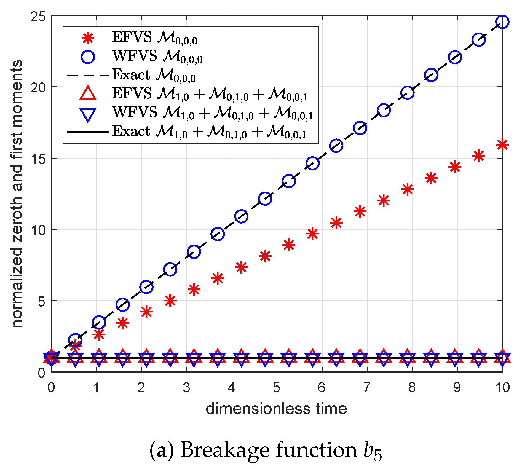
In the second instance, we choose two problems by setting the size-dependent selection function $S(x,y)=x+y$, along with the previously chosen particle daughter distribution functions $b_1$ and $b_2$. In this case, also the exact solutions are not available in the literature, however only the zeroth- and first-order moment functions can be calculated exactly. In both the cases, the moment functions are given as

$${\mathcal{M}}_{1,0}\left(t\right)+{\mathcal{M}}_{0,1}\left(t\right)=1,\mathrm{and}{\mathcal{M}}_{0,0}\left(t\right)=1+2t.$$

The following Figure 3a,b represent the efficiency of the WFV scheme over the EFV scheme to estimate the zeroth- and the first-order moments. It is observed that both the schemes obey the volume conservation laws with high accuracy, but the WFV scheme is highly accurate to predict the evolution of total number of particles. Table 4 and Table 5 represent the relative errors over different grid points at time $t=10$.

Figure 3. Comparison of zeroth- and first-order moments with selection function $S=x+y$, and breakage functions $b_1$, $b_2$.

Table 4. Relative error for the weighted moments at different grid points for the test case with $S=x+y$ and breakage function $b_1$ at $t=10$.

Grids	WFVS			EFVS
	${\mathcal{M}}_{0,0}\left(\mathit{t}\right)$	${\mathcal{M}}_{1,0}\left(\mathit{t}\right)+{\mathcal{M}}_{0,1}\left(\mathit{t}\right)$	CPU Time	${\mathcal{M}}_{0,0}\left(\mathit{t}\right)$	${\mathcal{M}}_{1,0}\left(\mathit{t}\right)+{\mathcal{M}}_{0,1}\left(\mathit{t}\right)$	CPU Time
10 × 10	9.9944 × 10${}^{-1}$	1.2589 × 10${}^{-1}$	2 s	9.9983 × 10${}^{-1}$	1.2589 × 10${}^{-1}$	1 s
15 × 15	9.9939 × 10${}^{-1}$	2.5119 × 10${}^{-1}$	5 s	9.9969 × 10${}^{-1}$	2.5119 × 10${}^{-1}$	2 s
20 × 20	9.9934 × 10${}^{-1}$	3.5481 × 10${}^{-1}$	11 s	9.9957 × 10${}^{-1}$	3.5481 × 10${}^{-1}$	5 s

Table 5. Relative error for the weighted moments at different grid points for the test case with $S=x+y$ and breakage function $b_2$ at $t=10$.

Grids	WFVS			EFVS
	${\mathcal{M}}_{0,0}\left(\mathit{t}\right)$	${\mathcal{M}}_{1,0}\left(\mathit{t}\right)+{\mathcal{M}}_{0,1}\left(\mathit{t}\right)$	CPU Time	${\mathcal{M}}_{0,0}\left(\mathit{t}\right)$	${\mathcal{M}}_{1,0}\left(\mathit{t}\right)+{\mathcal{M}}_{0,1}\left(\mathit{t}\right)$	CPU Time
10 × 10	1.8625 × 10${}^{-1}$	3.5481 × 10${}^{-1}$	21 s	7.6213 × 10${}^{-1}$	3.5481 × 10${}^{-1}$	10 s
15 ×15	1.8658 × 10${}^{-1}$	3.8986 × 10${}^{-1}$	28 s	5.2710 × 10${}^{-1}$	3.8986 × 10${}^{-1}$	17 s
20 × 20	1.8698 × 10${}^{-1}$	4.3652 × 10${}^{-1}$	41 s	2.7194 × 10${}^{-1}$	4.3652 × 10${}^{-1}$	21 s

4.1.2. Hypervolume Conservation Problems

In this part, the considered breakage functions b should satisfy the hypervolume conservation rule (8). In this regard, we choose the following breakage functions

$$\begin{array}{c}\hfill b_3(x,y|x^{\prime },y^{\prime })=\frac{4}{x^{\prime }{y}^{\prime }},\mathrm{and}{b}_4(x,y|x^{\prime },y^{\prime })=\frac{x^{\prime }\delta (x-x^{\prime })+y^{\prime }\delta (y-y^{\prime })}{x^{\prime }{y}^{\prime }}.\end{array}$$

(55)

The breakage function $b_3$ is independent of the daughter-particle size, whereas $b_4$ represents the particle breakage along the longer side of the rectangular structure. Similar to the examples of volume conservation models, we choose two types of selection functions: (i) size-independent kernels $S(x,y)=1$, and (ii) size-dependent kernels $S(x,y)=xy$.

Like before, the exact solutions are not available in the literature, however we can calculate three moment functions exactly, and they are given in Table 6.

Table 6. Exact moment functions for $S=1$ and breakage functions $b_3$, $b_4$.

Selection Function	Breakage Function	Exact Moments
$S(x,y)=1$	${\displaystyle b_3(x,y|x^{\prime },y^{\prime })=\frac{4}{x^{\prime }{y}^{\prime }}}$	${\mathcal{M}}_{k,l}\left(t\right)={\mathcal{M}}_{k,l}\left(0\right)exp\left[\left(\frac{4}{(k+1)(l+1)}-1\right)t\right]$
$S(x,y)=1$	${\displaystyle b_4\left(x,y|x^{\prime },y^{\prime }\right)=\frac{x^{\prime }\delta (x-x^{\prime })+y^{\prime }\delta (y-y^{\prime })}{x^{\prime }{y}^{\prime }}}$	${\mathcal{M}}_{1,1}\left(t\right)=1,{\mathcal{M}}_{0,0}\left(t\right)=exp\left(t\right)$, ${\mathcal{M}}_{1,0}\left(t\right)+{\mathcal{M}}_{0,1}\left(t\right)=exp\left(t/2\right)$

In Figure 4a, we plot the zeroth- and the cross-moment functions and observe that the new WFV scheme predicts the corresponding moments with high accuracy. On the other hand, we plot the first-order moment in Figure 4b. In this case also, the weighted scheme exhibits high accuracy to estimate the moment compared to the standard model. In Figure 4b, we take the the axes in loglog scale for a distinct visibility of the plots. In this problem, Figure 4c represents the comparison of hypervolume distribution functions with the numerical values obtained from the two schemes. We follow the flat pictorial representation to plot the hypervolume distribution as presented in [32]. For the other problems, only the exact moment functions can be calculated for comparison with the numerical models.

Figure 4. Comparison of different moments with selection function $S=1$, and breakage function $b_3$.

The relative errors over different grid points are presented at Table 7.

Table 7. Relative error for the weighted moments at different grid points for the test case with $S=1$ and breakage functions $b_3$ at $t=10$.

Grids	WFVS				EFVS
	${\mathcal{M}}_{0,0}\left(\mathit{t}\right)$	${\mathcal{M}}_{1,0}\left(\mathit{t}\right)+{\mathcal{M}}_{0,1}\left(\mathit{t}\right)$	${\mathcal{M}}_{1,1}\left(\mathit{t}\right)$	CPU Time	${\mathcal{M}}_{0,0}\left(\mathit{t}\right)$	${\mathcal{M}}_{1,0}\left(\mathit{t}\right)+{\mathcal{M}}_{0,1}\left(\mathit{t}\right)$	${\mathcal{M}}_{1,1}\left(\mathit{t}\right)$	CPU Time
10 × 10	1.9052 × 10${}^{-8}$	9.5538	6.8292 × 10${}^{-1}$	6 s	1.0000	2.2013 × 10${}^1$	6.8309 × 10${}^{-1}$	2 s
15 × 15	1.7344 × 10${}^{-8}$	6.5432	6.0859 × 10${}^{-1}$	19 s	1.0000	2.1890 × 10${}^1$	6.0863 × 10${}^{-1}$	8 s
20 × 20	1.6682 × 10${}^{-8}$	4.9080	5.4110 × 10${}^{-1}$	32 s	1.0000	2.1353 × 10${}^1$	5.4112 × 10${}^{-1}$	14 s

In the second instance, we consider the size-dependent selection function $S(x,y)=1$ and $b_4$ as the daughter distribution function. The exact solution is not available for this problem, but we can evaluate the zeroth and cross moments exactly. From the Figure 5 and Table 8, we can see that the newly proposed WFV scheme predicts the moments with high accuracy.

Figure 5. Comparison of different moments with selection function $S=1$, and breakage function $b_4$.

Table 8. Relative error for the weighted moments at different grid points for the test case with $S=1$ and breakage functions $b_4$ at $t=10$.

Grids	WFVS				EFVS
	${\mathcal{M}}_{0,0}\left(\mathit{t}\right)$	${\mathcal{M}}_{1,0}\left(\mathit{t}\right)+{\mathcal{M}}_{0,1}\left(\mathit{t}\right)$	${\mathcal{M}}_{1,1}\left(\mathit{t}\right)$	CPU Time	${\mathcal{M}}_{0,0}\left(\mathit{t}\right)$	${\mathcal{M}}_{1,0}\left(\mathit{t}\right)+{\mathcal{M}}_{0,1}\left(\mathit{t}\right)$	${\mathcal{M}}_{1,1}\left(\mathit{t}\right)$	CPU Time
10 × 10	4.5211 × 10${}^{-10}$	2.2694	6.8309 × 10${}^{-1}$	4 s	9.9946 × 10${}^{-1}$	1.4453 × 10${}^2$	6.8309 × 10${}^{-1}$	2 s
15 × 15	2.2036 × 10${}^{-10}$	2.8531 × 10${}^{-1}$	6.0863 × 10${}^{-1}$	10 s	9.9489 × 10${}^{-1}$	1.3513 × 10${}^2$	6.0863 × 10${}^{-1}$	5 s
20 × 20	1.6944 × 10${}^{-10}$	4.7015 × 10${}^{-2}$	5.4112 × 10${}^{-1}$	22 s	9.7532 × 10${}^{-1}$	1.1682 × 10${}^2$	5.4112 × 10${}^{-1}$	10 s

Next, we consider two problems with size-dependent selection function $S(x,y)=xy$ and the breakage functions $b_3$ and $b_4$. Only the zeroth- and first-order moment functions can be calculated in closed form, and are given in the Table 9.

Table 9. Exact moment functions for $S=xy$ and breakage functions $b_3$, $b_4$.

Selection Function	Breakage Function	Exact Moments
$S(x,y)=xy$	${\displaystyle b_3(x,y|x^{\prime },y^{\prime })=\frac{4}{x^{\prime }{y}^{\prime }}}$	${\mathcal{M}}_{1,1}\left(t\right)=1$, ${\mathcal{M}}_{0,0}\left(t\right)=1+3t$
$S(x,y)=xy$	${\displaystyle b_4\left(x,y|x^{\prime },y^{\prime }\right)=\frac{x^{\prime }\delta (x-x^{\prime })+y^{\prime }\delta (y-y^{\prime })}{x^{\prime }{y}^{\prime }}}$	${\mathcal{M}}_{1,1}\left(t\right)=1$, ${\mathcal{M}}_{0,0}\left(t\right)=1+t$

Numerical evaluation of the moments using the WFV and EFV schemes are presented in Figure 6 and Table 10 and Table 11. The improved accuracy of the new scheme is observed.

Figure 6. Comparison of different moments with selection function $S=xy$, and breakage functions $b_3$, $b_4$.

Table 10. Relative error for the weighted moments at different grid points for the test case with $S=xy$ and breakage function $b_3$ at $t=10$.

Grids	WFVS			EFVS
	${\mathcal{M}}_{0,0}\left(\mathit{t}\right)$	${\mathcal{M}}_{1,1}\left(\mathit{t}\right)$	CPU Time	${\mathcal{M}}_{0,0}\left(\mathit{t}\right)$	${\mathcal{M}}_{1,1}\left(\mathit{t}\right)$	CPU Time
10 × 10	5.4678 × 10${}^{-1}$	6.8309 × 10${}^{-1}$	1 s	8.8071 × 10${}^{-1}$	6.8309 × 10${}^{-1}$	1 s
15 × 15	5.5130 × 10${}^{-1}$	6.0863 × 10${}^{-1}$	1 s	8.0374 × 10${}^{-1}$	6.0863 × 10${}^{-1}$	1 s
20 × 20	5.5418 × 10${}^{-1}$	5.4112 × 10${}^{-1}$	3 s	7.4013 × 10${}^{-1}$	5.4112 × 10${}^{-1}$	2 s

Table 11. Relative error for the weighted moments at different grid points for the test case with $S=xy$ and breakage function $b_4$ at $t=10$.

Grids	WFVS			EFVS
	${\mathcal{M}}_{0,0}\left(\mathit{t}\right)$	${\mathcal{M}}_{1,1}\left(\mathit{t}\right)$	CPU Time	${\mathcal{M}}_{0,0}\left(\mathit{t}\right)$	${\mathcal{M}}_{1,1}\left(\mathit{t}\right)$	CPU Time
10 × 10	3.3663 × 10${}^{-1}$	6.8309 × 10${}^{-1}$	1 s	7.6014 × 10${}^{-1}$	6.8309 × 10${}^{-1}$	1 s
15 × 15	1.3416 × 10${}^{-1}$	6.0863 × 10${}^{-1}$	1 s	7.9649 × 10${}^{-1}$	6.0863 × 10${}^{-1}$	1 s
20 × 20	5.4011 × 10${}^{-1}$	5.4112 × 10${}^{-1}$	2 s	7.4013 × 10${}^{-1}$	5.4112 × 10${}^{-1}$	2 s

4.2. Three-Dimensional Examples

Volume conservative problems: In this section, we consider two test problems with size-dependent selection function $S\left(\mathbf{y}\right)=\varphi \left(\mathbf{y}\right)$. The three-dimensional extension of the above-mentioned breakage functions $b_1$ and $b_2$, that is,

$$b_5\left(\mathbf{x}|\mathbf{y}\right)=\frac{2}{\psi \left(\mathbf{y}\right)},\mathrm{and}{b}_6\left(\mathbf{x}|\mathbf{y}\right)=2\delta \left(x_1-\frac{y_1}{2}\right)\delta \left(x_2-\frac{y_2}{2}\right)\delta \left(x_3-\frac{y_3}{2}\right)$$

are considered here. Like before, we can only calculate the zeroth and first moments exactly and they are given in the following Table 12.

Table 12. Exact moment functions for $S=\varphi \left(\mathbf{y}\right)$ and breakage functions $b_5$, $b_6$.

Selection Function	Breakage Function	Exact Moments
$S\left(\mathbf{y}\right)=\varphi \left(\mathbf{y}\right)$	${\displaystyle b_5\left(\mathbf{x}|\mathbf{y}\right)=\frac{2}{\psi \left(\mathbf{y}\right)}}$	${\mathcal{M}}_{k_1,k_2,k_3}\left(t\right)={\mathcal{M}}_{k_1,k_2,k_3}\left(0\right)exp\left[\left(\frac{8}{k_1{k}_2{k}_3}-1\right)t\right]$
$S\left(\mathbf{y}\right)=\varphi \left(\mathbf{y}\right)$	$b_6\left(\mathbf{x}|\mathbf{y}\right)=2\delta \left(x_1-\frac{y_1}{2}\right)\delta \left(x_2-\frac{y_2}{2}\right)\delta \left(x_3-\frac{y_3}{2}\right)$	${\mathcal{M}}_{1,0,0}\left(t\right)+{\mathcal{M}}_{1,0,0}\left(t\right)+{\mathcal{M}}_{1,0,0}\left(t\right)=1$, ${\mathcal{M}}_{0,0}\left(t\right)=1+3t$

From Figure 7 and Table 13 and Table 14, we can observe that the WFV scheme estimates the moment functions more accurately as compared to the EFV scheme.

Figure 7. Comparison of zeroth- and first-order moments with selection function $S=\varphi \left(\mathbf{x}\right)$, and different breakage functions $b_5$, $b_6$.

Table 13. Relative error for the weighted moments at different grid points for the test case with $S=\varphi \left(\mathbf{x}\right)$ and breakage function $b_5$ at $t=10$.

Grids	WFVS			EFVS
	${\mathcal{M}}_{0,0,0}\left(\mathit{t}\right)$	${\mathcal{M}}_{1,0,0}\left(\mathit{t}\right)+{\mathcal{M}}_{0,1,0}\left(\mathit{t}\right)+{\mathcal{M}}_{0,0,1}\left(\mathit{t}\right)$	CPU Time	${\mathcal{M}}_{0,0,0}\left(\mathit{t}\right)$	${\mathcal{M}}_{1,0,0}\left(\mathit{t}\right)+{\mathcal{M}}_{0,1,0}\left(\mathit{t}\right)+{\mathcal{M}}_{0,0,1}\left(\mathit{t}\right)$	CPU Time
10 × 10 × 10	9.9302 × 10${}^{-15}$	6.8884 × 10${}^{-1}$	52 s	7.1010 × 10${}^{-1}$	6.8884 × 10${}^{-1}$	34 s
15 × 15 × 15	1.1192 × 10${}^{-15}$	8.0464 × 10${}^{-1}$	198 s	5.7788 × 10${}^{-1}$	8.0464 × 10${}^{-1}$	78 s
20 × 20 × 20	2.8756 × 10${}^{-16}$	8.7678 × 10${}^{-1}$	505 s	5.0076 × 10${}^{-1}$	8.7678 × 10${}^{-1}$	292 s

Table 14. Relative error for the weighted moments at different grid points for the test case with $S=\varphi \left(\mathbf{x}\right)$ and breakage function $b_6$ at $t=10$.

Grids	WFVS			EFVS
	${\mathcal{M}}_{0,0,0}\left(\mathit{t}\right)$	${\mathcal{M}}_{1,0,0}\left(\mathit{t}\right)+{\mathcal{M}}_{0,1,0}\left(\mathit{t}\right)+{\mathcal{M}}_{0,0,1}\left(\mathit{t}\right)$	CPU Time	${\mathcal{M}}_{0,0,0}\left(\mathit{t}\right)$	${\mathcal{M}}_{1,0,0}\left(\mathit{t}\right)+{\mathcal{M}}_{0,1,0}\left(\mathit{t}\right)+{\mathcal{M}}_{0,0,1}\left(\mathit{t}\right)$	CPU Time
10 × 10 × 10	3.7623 × 10${}^{-1}$	1.8500 × 10${}^{-1}$	73 s	2.9725 × 10${}^{-1}$	5.0569 × 10${}^{-1}$	36 s
15 × 15 × 15	1.4588 × 10${}^{-1}$	3.5055 × 10${}^{-2}$	294 s	2.0743 × 10${}^{-1}$	3.8846 × 10${}^{-1}$	139 s
20 × 20 × 20	9.6814 × 10${}^{-2}$	3.0046 × 10${}^{-2}$	660 s	1.1094 × 10${}^{-1}$	1.9000 × 10${}^{-1}$	335 s

Hypervolume conservation: In this instance, we consider the size-independent daughter distribution function ${\displaystyle b_7\left(\mathbf{x}|\mathbf{y}\right)=\frac{8}{\psi \left(\mathbf{y}\right)}}$ along with the constant selection $S=1$ and size-dependent selection $S\left(\mathbf{y}\right)=\psi \left(\mathbf{y}\right)$. The exact moments are calculated in the Table 15.

Table 15. Exact moment functions for $S\left(\mathbf{y}\right)=1$, $S=\psi \left(\mathbf{y}\right)$ and breakage function $b_7$.

Selection Function	Breakage Function	Exact Moments
$S\left(\mathbf{y}\right)=1$	${\displaystyle b_7\left(\mathbf{x}|\mathbf{y}\right)=\frac{8}{\psi \left(\mathbf{y}\right)}}$	${\mathcal{M}}_{0,0,0}\left(t\right)=exp\left(7t\right)$, ${\mathcal{M}}_{1,1,1}\left(t\right)=1$, ${\mathcal{M}}_{1,0,0}\left(t\right)+{\mathcal{M}}_{0,1,0}\left(t\right)+{\mathcal{M}}_{0,0,1}\left(t\right)=exp\left(3t\right)$
$S\left(\mathbf{y}\right)=\psi \left(\mathbf{y}\right)$	${\displaystyle b_7\left(\mathbf{x}|\mathbf{y}\right)=\frac{8}{\psi \left(\mathbf{y}\right)}}$	${\mathcal{M}}_{0,0,0}\left(t\right)=1+7t$, ${\mathcal{M}}_{1,1,1}\left(t\right)=1$

Figure 8 and Table 16 exhibit the improved accuracy obtained from the WFV scheme over the standard scheme to predict the above mentioned three moments.

Figure 8. Comparison of zeroth- and first-order moments with selection function $S=1$, and breakage functions $b_7$.

Table 16. Relative error for the weighted moments at different grid points for the test case with $S=1$ and breakage functions $b_7$ at $t=10$.

Grids	WFVS				EFVS
	${\mathcal{M}}_{0,0,0}\left(\mathit{t}\right)$	${\mathcal{M}}_{1,0,0}\left(\mathit{t}\right)+{\mathcal{M}}_{0,1,0}\left(\mathit{t}\right)+{\mathcal{M}}_{0,0,1}\left(\mathit{t}\right)$	${\mathcal{M}}_{1,1,1}\left(\mathit{t}\right)$	CPU Time	${\mathcal{M}}_{0,0,0}\left(\mathit{t}\right)$	${\mathcal{M}}_{1,0,0}\left(\mathit{t}\right)+{\mathcal{M}}_{0,1,0}\left(\mathit{t}\right)+{\mathcal{M}}_{0,0,1}\left(\mathit{t}\right)$	${\mathcal{M}}_{1,1,1}\left(\mathit{t}\right)$	CPU Time
10 × 10 × 10	5.8045 × 10${}^{-8}$	2.8046	1.5759 × 10${}^{-1}$	164 s	1.0000	1.0013 × 10${}^1$	8.2160 × 10${}^{-1}$	44 s
15 × 15 × 15	5.7040 × 10${}^{-8}$	1.7385 × 10${}^{-1}$	3.7535 × 10${}^{-2}$	605 s	1.0000	1.0000	7.8233 × 10${}^{-1}$	272 s
20 × 20 × 20	5.6751 × 10${}^{-8}$	1.4056 × 10${}^{-1}$	1.9838 × 10${}^{-2}$	1500 s	1.0000	9.9999 × 10${}^{-1}$	7.5516 × 10${}^{-1}$	650 s

On the other hand, Figure 9 and Table 17 represent the comparison of the above moments as predicted by the WFV and EFV schemes.

Figure 9. Comparison of zeroth and cross moments with selection function $S=\psi \left(\mathbf{x}\right)$, and breakage function $b_7$.

Table 17. Relative error for the weighted moments at different grid points for the test case with $S=\psi \left(\mathbf{x}\right)$ and breakage function $b_7$ at $t=10$.

Grids	WFVS			EFVS
	${\mathcal{M}}_{0,0,0}\left(\mathit{t}\right)$	${\mathcal{M}}_{1,1,1}\left(\mathit{t}\right)$	CPU Time	${\mathcal{M}}_{0,0,0}\left(\mathit{t}\right)$	${\mathcal{M}}_{1,1,1}\left(\mathit{t}\right)$	CPU Time
10 × 10 × 10	3.9509 × 10${}^{-16}$	8.2160 × 10${}^{-1}$	5 s	8.0112 × 10${}^{-1}$	8.2160 × 10${}^{-1}$	3 s
15 × 15 × 15	6.5640 × 10${}^{-16}$	7.8233 × 10${}^{-1}$	24 s	7.1237 × 10${}^{-1}$	7.8233 × 10${}^{-1}$	11 s
20 × 20 × 20	9.7932 × 10${}^{-16}$	7.5516 × 10${}^{-1}$	70 s	6.4883 × 10${}^{-1}$	7.5516 × 10${}^{-1}$	30 s

5. Conclusions

In this article, we have proposed finite volume schemes for solving multidimensional fragmentation problems. In addition to the one-dimensional scheme of [23], it is also extended in the multidimensional setup. It is observed that a careful reconstruction of the standard multidimensional scheme leads to the development of very accurate schemes. The newly proposed schemes obey the conservation laws and also predict several physical moment functions with high accuracy. Several empirical test problems in two- and three-dimensions are collected from the literature to validate the efficiency of the new schemes.

References

- Hauk, T.; Bonaccurso, E.; Roisman, I.; Tropea, C. Ice crystal impact onto a dry solid wall. Particle fragmentation. Proc. R. Soc. A Math. Phys. Eng. Sci. 2015, 471, 20150399. [Google Scholar] [CrossRef]
- Kang, D.H.; Ko, C.K.; Lee, D.H. Attrition characteristics of iron ore by an air jet in gas-solid fluidized beds. Powder Technol. 2017, 316, 69–78. [Google Scholar] [CrossRef]
- Cavalcanti, P.P.; de Carvalho, R.M.; Anderson, S.; da Silveira, M.W.; Tavares, L.M. Surface breakage of fired iron ore pellets by impact. Powder Technol. 2019, 342, 735–743. [Google Scholar] [CrossRef]
- Fulchini, F.; Ghadiri, M.; Borissova, A.; Amblard, B.; Bertholin, S.; Cloupet, A.; Yazdanpanah, M. Development of a methodology for predicting particle attrition in a cyclone by CFD-DEM. Powder Technol. 2019, 357, 21–32. [Google Scholar] [CrossRef]
- Jain, D.; Kuipers, J.; Deen, N.G. Numerical study of coalescence and breakup in a bubble column using a hybrid volume of fluid and discrete bubble model approach. Chem. Eng. Sci. 2014, 119, 134–146. [Google Scholar] [CrossRef]
- Li, L.; Kang, Y.T. Effects of bubble coalescence and breakup on CO2 absorption performance in nanoabsorbents. J. CO2 Util. 2020, 39, 101170. [Google Scholar] [CrossRef]
- Foroushan, H.K.; Jakobsen, H.A. On the Dynamics of Fluid Particle Breakage Induced by Hydrodynamic Instabilities: A Review of Modelling Approaches. Chem. Eng. Sci. 2020, 2020, 115575. [Google Scholar] [CrossRef]
- Herø, E.H.; Forgia, N.L.; Solsvik, J.; Jakobsen, H.A. Determination of Breakage Parameters in Turbulent Fluid-Fluid Breakage. Chem. Eng. Technol. 2019, 42, 903–909. [Google Scholar] [CrossRef]
- Yang, W.; Luo, Z.; Gu, Y.; Liu, Z.; Zou, Z. Simulation of bubbles behavior in steel continuous casting mold using an Euler-Lagrange framework with modified bubble coalescence and breakup models. Powder Technol. 2020, 361, 769–781. [Google Scholar] [CrossRef]
- Nakach, M.; Authelin, J.R.; Chamayou, A.; Dodds, J. Comparison of various milling technologies for grinding pharmaceutical powders. Int. J. Miner. Process. 2004, 74, S173–S181. [Google Scholar] [CrossRef]
- Flach, F.; Konnerth, C.; Peppersack, C.; Schmidt, J.; Damm, C.; Breitung-Faes, S.; Peukert, W.; Kwade, A. Impact of formulation and operating parameters on particle size and grinding media wear in wet media milling of organic compounds– A case study for pyrene. Adv. Powder Technol. 2016, 27, 2507–2519. [Google Scholar] [CrossRef]
- Braig, V.; Konnerth, C.; Peukert, W.; Lee, G. Enhanced dissolution of naproxen from pure-drug, crystalline nanoparticles: A case study formulated into spray-dried granules and compressed tablets. Int. J. Pharm. 2019, 554, 54–60. [Google Scholar] [CrossRef]
- Sauvageot, H.; Koffi, M. Multimodal raindrop size distributions. J. Atmos. Sci. 2000, 57, 2480–2492. [Google Scholar] [CrossRef]
- Fuerstenau, D.; De, A.; Kapur, P. Linear and nonlinear particle breakage processes in comminution systems. Int. J. Miner. Process. 2004, 74, S317–S327. [Google Scholar] [CrossRef]
- Oddershede, L.; Dimon, P.; Bohr, J. Self-organized criticality in fragmenting. Phys. Rev. Lett. 1993, 71, 3107. [Google Scholar] [CrossRef]
- Ishii, T.; Matsushita, M. Fragmentation of long thin glass rods. J. Phys. Soc. Jpn. 1992, 61, 3474–3477. [Google Scholar] [CrossRef]
- Lee, K.F.; Dosta, M.; McGuire, A.D.; Mosbach, S.; Wagner, W.; Heinrich, S.; Kraft, M. Development of a multi-compartment population balance model for high-shear wet granulation with discrete element method. Comput. Chem. Eng. 2017, 99, 171–184. [Google Scholar] [CrossRef]
- Maslov, D. Absence of self-averaging in shattering fragmentation processes. Phys. Rev. Lett. 1993, 71, 1268. [Google Scholar] [CrossRef] [PubMed]
- Rodgers, G.; Hassan, M. Fragmentation of particles with more than one degree of freedom. Phys. Rev. E 1994, 50, 3458. [Google Scholar] [CrossRef]
- Singh, P.; Hassan, M. Kinetics of multidimensional fragmentation. Phys. Rev. E 1996, 53, 3134. [Google Scholar] [CrossRef] [PubMed]
- Hernández, G. Discrete model for fragmentation with random stopping. Phys. A Stat. Mech. Its Appl. 2001, 300, 13–24. [Google Scholar] [CrossRef]
- Saha, J.; Bück, A. Improved accuracy and convergence analysis of finite volume methods for particle fragmentation models. Math. Methods Appl. Sci. 2021, 44, 1913–1930. [Google Scholar] [CrossRef]
- Kumar, R.; Kumar, J. Numerical simulation and convergence analysis of a finite volume scheme for solving general breakage population balance equations. Appl. Math. Comput. 2013, 219, 5140–5151. [Google Scholar] [CrossRef]
- Boyer, D.; Tarjus, G.; Viot, P. Exact solution and multifractal analysis of a multivariable fragmentation model. J. Phys. I 1997, 7, 13–38. [Google Scholar] [CrossRef][Green Version]
- Nandanwar, M.N.; Kumar, S. A new discretization of space for the solution of multi-dimensional population balance equations: Simultaneous breakup and aggregation of particles. Chem. Eng. Sci. 2008, 63, 3988–3997. [Google Scholar] [CrossRef]
- Kumar, J.; Saha, J.; Tsotsas, E. Development and convergence analysis of a finite volume scheme for solving breakage equation. SIAM J. Numer. Anal. 2015, 53, 1672–1689. [Google Scholar] [CrossRef]
- Buffo, A.; Alopaeus, V. Solution of bivariate population balance equations with high-order moment-conserving method of classes. Comput. Chem. Eng. 2016, 87, 111–124. [Google Scholar] [CrossRef]
- Saha, J.; Kumar, J.; Heinrich, S. On the approximate solutions of fragmentation equations. Proc. R. Soc. A Math. Phys. Eng. Sci. 2018, 474, 20170541. [Google Scholar] [CrossRef]
- Saha, J.; Das, N.; Kumar, J.; Bück, A. Numerical solutions for multidimensional fragmentation problems using finite volume methods. Kinet. Relat. Model. 2019, 12, 79–103. [Google Scholar] [CrossRef]
- Ziff, R.M.; McGrady, E. The kinetics of cluster fragmentation and depolymerisation. J. Phys. A Math. Gen. 1985, 18, 3027. [Google Scholar] [CrossRef]
- Ziff, R.M. New solutions to the fragmentation equation. J. Phys. A Math. Gen. 1991, 24, 2821. [Google Scholar] [CrossRef]
- Chakraborty, J.; Kumar, S. A new framework for solution of multidimensional population balance equations. Chem. Eng. Sci. 2007, 62, 4112–4125. [Google Scholar] [CrossRef]
Publisher’s Note: MDPI stays neutral with regard to jurisdictional claims in published maps and institutional affiliations. |
© 2021 by the authors. Licensee MDPI, Basel, Switzerland. This article is an open access article distributed under the terms and conditions of the Creative Commons Attribution (CC BY) license (http://creativecommons.org/licenses/by/4.0/).