Abstract
While researchers and practitioners may seamlessly develop methods of detecting outliers in control charts under a univariate setup, detecting and screening outliers in multivariate control charts pose serious challenges. In this study, we propose a robust multivariate control chart based on the Stahel-Donoho robust estimator (SDRE), whilst the process parameters are estimated from phase-I. Through intensive Monte-Carlo simulation, the study presents how the estimation of parameters and presence of outliers affect the efficacy of the Hotelling T2 chart, and then how the proposed outlier detector brings the chart back to normalcy by restoring its efficacy and sensitivity. Run-length properties are used as the performance measures. The run length properties establish the superiority of the proposed scheme over the default multivariate Shewhart control charting scheme. The applicability of the study includes but is not limited to manufacturing and health industries. The study concludes with a real-life application of the proposed chart on a dataset extracted from the manufacturing process of carbon fiber tubes.
1. Introduction
Outliers are those observations at both extremes, which do not follow the majority of observations pattern in a dataset. Outlier detection is of concern in data analysis and scientific areas, of which statistical process control (SPC) is not an exemption [1]. This is because outliers have a major influence on any statistical analysis as they increase the error variance, reduce the power of statistical tests, and cause bias in estimation, hence leading to incorrect inferences and conclusions, and sometimes, ending with deadly decisions, take the health sector as an example. With little percentage and magnitude present in data (big or small), outliers will grossly distort the performance and analysis of the data. Therefore, the art of outlier detection is a prominent and important aspect of data analysis, even more so now that more and more data are being analyzed simultaneously, such as with multivariate control charting.
Control charts are the most widely used tool amongst the seven tools of SPC [2]. Their vast applicability in different fields and sectors give them an edge over other tools of SPC for process monitoring. Control charts, however, can have a univariate or multivariate setup, a memory or memory-less type, and/or monitoring location or dispersion in an ongoing process. Readers are referred to [2] for more information about control charts and their types. Furthermore, control charts are of two stages: phase-I (the prospective stage) and phase-II (the retrospective stage). The process parameters are used to set the chart’s control limits in phase-I. Moreover, if the process parameters are unknown, they are estimated with some preliminary samples, whereas the monitoring and correction of unnatural causes of variation occur in the retrospective stage. The choice and amount of preliminary sample employed in estimating the unknown parameters in phase-I vary among practitioners and as result affect the performance of the chart in the monitoring stage. These samples often contain some unusual observations and outliers, which exert a disproportionate pull on the parameter estimated, making the chart less efficient in detecting anomalies. The multivariate Shewhart chart that has been studied in this paper is a memory-less type for monitoring location parameters, while the process parameters are known and estimated from phase-I samples. Over the years, SPC researchers have investigated the effect of parameter estimation on control charts in both univariate and multivariate setups. To mention a few, reference [3] gave an up-to-date review on parameter estimation effects on control charts. Saleh et al. [4] evaluated the parameter estimation’s effect on an exponentially weighted moving average (EWMA) control chart with its run length properties. A similar study was conducted by Jones [5].
Many research works in the literature have studied outlier detection in the univariate setup, some of which are applied to control charts in the univariate setup. References [6,7,8] have independently proposed outlier detection models in the univariate setup of control charts either for location or dispersion monitoring. They found that the control charts based on detection models require fewer phase-I samples to detect anomalies, as these charts are quicker and more sensitive to contamination. Guarnieri et al. [9] developed control charts for individual observation and exponentially weighted moving averages based on residues to detect outliers in autoregressive models. Bakar et al. [10] also conducted a comparative study for outlier detection techniques in control charts with application in data mining. As Vidmar and Blagus [11] applied different outlier detection approaches to healthcare quality monitoring. Zhang and Albin [12] employed a chi-square chart method for detecting outliers in complex profiles. Other research in this direction include, among others, [13,14]. While there are models for detecting multivariate outliers, few of them have been applied to SPC. Examples include the robust multivariate control chart for outlier detection by Fan et al. [15] and robust estimates, residuals, and outlier detection with multi-response data by Gnanadesikan and Kettenring [16]. The authors of [17] considered minimum volume ellipsoid (MVE) and/or weighted mean vector and mean square successive differences (WD) to decrease the impact of outliers on multivariate control charts. Hubert et al. [18] reviewed the minimum covariance determinant (MCD) methods and their extension as competent tools for outlier detection. Other researchers have approached the outlier detection problem with robust multivariate estimators. The pioneer of this idea was Stahel [19] where he studied the breakdown of covariance estimators; Maronna and Yohai [20] further extended the research of Stahel. Rousseeuw and Hubert [21] also studied the robust multivariate location and scatter estimators. Similar studies include but are not limited to [22,23,24].
In the aforementioned references, none of the studies that applied multivariate robust estimators to control charts have focused on detecting and screening outliers of the phase-I samples. Therefore, this paper focuses on detecting multivariate outliers in the multivariate Shewhart control chart. It employs a Stahel-Donoho robust estimator incorporated with the Mahalanobis distance for detecting and screening out the outlying observations in the preliminary samples, from which the process parameters are estimated. This paper reports the effect of parameter estimations on a multivariate Shewhart chart’s control limits and performance. Reporting parameter estimations’ effect is not the main goal of this study; however, it helps readers to better understand the positive impact of the outlier detection process.
The remainder of this article is organized as follows. Section 2 entails the methodology with an insight to the multivariate Shewhart control chart when the process parameters are known and estimated, the presence of outliers in the preliminary samples, and the proposed multivariate outlier detection process. Results and discussion appear in Section 3, while Section 4 gives an illustrative example with a real-life dataset extracted from the manufacturing process of carbon fiber tubes. Section 5 concludes the study with a summary of the findings and future recommendations.
2. Methodology
The aim of this study is to detect and screen outliers of the m preliminary samples employed for parameter estimation, especially when the samples are outlier prone. This section explains in detail the multivariate Shewhart control chart for location monitoring, both when the parameters are known and estimated from phase-I preliminary samples. Then it demonstrates the effect of practitioners’ variability in the samples employed for estimation, and its effect on the chart’s performance. In addition, this section presents how outliers in those samples distort the chart’s efficacy and become less sensitive, then concludes the section with the proposed outlier detection-based multivariate Shewhart chart, and its application on a real-life data set extracted from the carbon fiber tubes manufacturing industry.
2.1. Multivariate Shewhart Control Chart
Let , a vector of p-correlated quality characteristics, each of size n subgroups, drawn from a p-variate normal distribution be the characteristic of interest for monitoring in a multivariate process. The probability distribution function of X is given as follows:
The resulting multivariate Shewhart chart statistic termed Hotelling T2, for monitoring the location parameter of the random process X, is given as follows:
where is the mean vector of the ith observation, n is the sample size, and
is the mean vector and variance-covariance matrix of the process. The chart signals an alarm when the statistic is plotted beyond the upper control limit (UCL) of the chart, i.e., ( This is the case when the process parameters () are known. However, when the parameters are unknown, they are estimated from m phase-I preliminary samples. The Hotelling T2 statistics then become
where and are the estimates of the in-control mean vector and variance-covariance matrix emerging from the phase-I samples. It is important to note that the amount of m phase-I sample and the choice of estimators employed for estimating the parameters vary amongst practitioners, hence the variability in the efficacy and performance of their charts. Subsequently, the corresponding UCL of the statistic in (3), for the monitoring stage, phase-II, is given as follows:
Again, if , the chart sends a signal, so the practitioner tends to the unnatural cause of variation. The ith observation on which a signal was sent is the run length. The run length is simply the number of observations plotted within the limit before recording the first out-of-control (OoC). With many iterations, run length becomes a variable whose properties will be used for evaluating the chart.
All this explains the traditional method for constructing the multivariate Shewhart chart for location monitoring. The next section establishes parameter estimation effects on the multivariate Shewhart chart. Section 2.3, on the other hand, reveals how the outliers emanating from the phase-I sample negatively affect the chart’s performance, while Section 2.4 highlights the need for incorporating multivariate robust estimators for outlier detection.
2.2. Effect of Practitioners’ Variabilities on the Multivariate Shewhart Chart
In this section, the study reveals how the practitioners’ variability in the choice of m samples affects the multivariate Shewhart chart’s performance. Through intensive Monte-Carlo simulation, we demonstrate how different m phase-I samples for estimating the unknown parameters play a vital role in the performance of the multivariate Shewhart chart as compared to the known parameter case. This study considers of 25, 100, and 500 to represent small, medium, and large samples, respectively. An algorithm was developed in R language to simulate the multivariate Shewhart chart defined in (2) for the known parameter case and in (3) for the unknown case. For the known case, it was assumed that the mean vector was zero, variances were unity, and the covariance was 50% (i.e., and ). With , the in-control (IC) average run length () corresponded to 370. While for the unknown cases, the process parameters were estimated from samples with sample mean vector and covariance matrix S. The algorithm also considered the OoC situations, when the mean vector increased over a range of shift . The first effect of estimation began with the UCL; the UCL varied as the m sample varied, to yield the nominal of 370 as in the known case. The simulation results are presented in Table 1 and Table 2. The detailed discussion of these results is in Section 3.

Table 1.
ARL and SDRL values of the multivariate Shewhart control chart with p = 2.
Table 2.
ARL and SDRL values of the multivariate Shewhart control chart with p = 3.
2.3. Effect of Outliers on the Multivariate Shewhart Control Chart with Estimated Parameters
Having noticed the estimation effect on the multivariate Shewhart chart’s performance in the previous section, we demonstrate how outliers in the m phase-I samples worsen the chart’s performance in the monitoring stage. To achieve this aim, we generated m phase-I samples from a mixed distribution, a(1 − θ)100% from the normal distribution and the remaining θ100% from a chi-square distribution with v degrees of freedom as follows:
where θ > 0 represents the percentage of outliers present in the data, ω ≥ 1 is the magnitude of the outliers, and represents the outlier added to the normal distribution. The study estimated the parameters and S from the m sample, and then computed the Hotelling T2 statistic as in (3). The same algorithm, process parameters, and control limits employed in Section 2.2 were used to compute the IC run length properties alone to observe the outliers’ effect. The results are presented in Table 3 and Table 4 for magnitudes ω = 1,2, respectively. With just of outliers (θ = 0.10), the increased by more than of its expected value when ω = 1 and close to 3000% when ω = 2.
Table 3.
ALR0 and SDRL0 values of the multivariate Shewhart control chart with outliers (ω = 1).
Table 4.
ALR0 and SDRL0 values of the multivariate Shewhart control chart with outliers (ω = 2).
The findings from the results in this section and the previous section suggest the following options:
- The m phase-I sample should be sufficiently increased until results similar to those of the known case are achieved.
- The process should prevent the occurrence of unnatural variations and outliers with smaller m phase-I samples
These options are practically impossible in real life scenarios, because increasing samples is typically uneconomical. More so, a process cannot be freed from variations with a natural or assignable cause. Hence, there is the need to incorporate robust multivariate estimators for better estimation and screening of the outliers.
2.4. Proposed Multivariate Shewhart Chart Based on Stahel-Donoho Robust Estimators (SDRE)
From the results in Table 3 and Table 4, it is apparent that increasing the m samples cannot suppress the negative impact of the outliers on the chart. Hence, there is a need to employ robust location and dispersion estimators as substitutes to the default and S that are not sensitive to outliers. Therefore, this study proposes a multivariate Shewhart chart based on the Stahel-Donoho robust estimator. Like any robust estimator, the SDRE estimators were able to retain their efficiency in the presence of outliers. This feature makes them able to detect the presence of outliers no matter how small or large the m samples are. Readers are referred to [25,26,27] for more information about the merits of robust estimators.
Stahel [19] and Donoho [22] were the first to develop a robust equivariant estimator of multivariate location and dispersion with a considerable high breakdown point of any p-variate multivariate data. However, it became well known with the analysis of Maronna and Yohai [20]. Maronna and Yohai [20] assumed to be a set of n data points in , and defined the “outlyingness” r for any as , where and μ() and σ() are the robust univariate location and dispersion statistics. The Stahel-Donoho robust estimators (SDRE), denoted as (t,V), are defined as weighted mean and weighted covariance matrix, each with weights of the form w(r), where wi is the weight function of each observation and inverse proportional to the “outlyingness” of the observation, r, obtained by considering all univariate projections of the data. Mathematically, SDRE is written as follows:
where . The SDRE is then used to estimate the process parameters from the m phase-I samples instead of and S. Furthermore, (t,V) estimators are employed in the Mahalanobis distance to screen out the potential outliers present in the m samples as in (7).
2.5. The Algorithm
This section explains in detail the algorithm and performance evaluation adopted in this study. The major performance measure of a control chart is the run length properties: average run length (ARL) and the standard deviation of the run length (SDRL). Through the Monte-Carlo simulation approach, the run length properties of both the IC ( and ) and OoC ( and ) of the scheme were computed. The following is the algorithm developed in R language to achieve this aim:
- Generate 106 random variables of p-variate quality characteristics, each of sample size n = 5 from a multivariate normal distribution to be monitored in the phase-II stage.
- (a) Known case: Define the mean vectors and covariance matrix, then proceed to step 3.(b) Unknown case: Generate some m phase-I samples from the same distributions to compute the default mean vector and covariance matrix estimators ( and S), then proceed to step 3 (see Section 2.2).(c) Unknown case with outliers: Generate some m phase-I samples from a mixed distribution as defined in (5), then compute the default mean vector and covariance matrix estimators ( and S) and then proceed to step 3 (see Section 2.3).(d) Unknown case with outliers screened: Generate some m phase-I samples from a mixed distribution as defined in (5), compute the SDRE (t,V) in (6), employ the SDRE to screen the outliers as explained in (7), and then compute and S of the remaining dataset after screening. Then, proceed to step 3 (see Section 2.4).
- Calculate the statistic in (2) for the known parameter case and (3) for the unknown cases, as the case may be.
- Plot the statistic against the control limit, UCL, until the first ith observation plots beyond UCL. For known cases, UCL = , while for the unknown cases, use the UCL defined in (4).
- Record the ith observation where the signal occurred as the run length.
- Repeat the steps from 1–5 for 105 iterations. Record the run length for each iteration. Then, calculate the average and standard deviation of the run length as ARL0 and SDRL0, respectively.The algorithm is summarized with a flowchart presented in Figure 1 for easy readability.
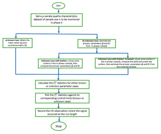 Figure 1. The flowchart of the methodology.
3. Results and Discussions
This section presents and discusses the results and findings of the methodologies explained in Section 2, in three categories: (a) the effect of practitioners’ variabilities on the chart, (b) the effect of outliers on the chart’s performance, and (c) the improvement of the proposed SDRE-based multivariate chart. The performance measure of this study was the run-length properties. The IC and were expected to be sufficiently large as the nominal = 370, while the OoC and were expected to be significantly small, implying the chart’s ability to quickly detect anomalies in the process.
3.1. Practitioners’ Variability Effect on Multivariate Shewhart Chart
Following the algorithm in Section 2.5, Table 1 and Table 2 contain the ARLs of the multivariate Shewhart chart for the known parameter case and the estimated parameters with and 3, respectively. The parameter estimation effect on the chart’s performance is evident from the ARL and SDRL values. The different m phase-I samples represent the variabilities in practitioners’ choice, ranging from small to medium to large. The larger the m samples, the better the chart’s performance as compared to the known case. When δ = 0, both the and were expected to cluster around the nominal value 370. The ARL values did so, but the SDRLs of the estimated parameter scenarios did not. They dispersed from 370, and the disparity became even wider as the m samples got smaller. Another major effect was how the charts with the estimated parameters were less sensitive to shift as their and imply. This effect also worsened as the m samples reduced (see Table 1 and Table 2).
3.2. Effect of Outliers on the Multivariate Shewhart Chart’s Performance
Table 3 and Table 4 depict the in-control and of the multivariate Shewhart chart from the mixed distribution in (5), with , some percentages of outliers , and the magnitude . Here, all values should be approximate to the nominal ARL of 370, since the environment was IC. When , it implies the absence of outliers in the process, so the ARL values for all different samples clustered around 370, while their SDRL values did not. It can be easily observed from the two tables that the outliers’ effect on the chart worsened as the percentage and magnitude of outliers increased. Also, the effect on the ARL values was more obvious as the sample increased, and vice-versa for the SDRL values. In general, there was more than a 600% increment in the ARL and SDRL values when and a more than 3000% increment when . All of these were due to less than 10% outliers in the data.
3.3. Improvement of the Proposed SDRE-Based Multivariate Shewhart Chart
Here, we present and discuss the results of the proposed multivariate Shewhart chart based on SDRE and Mahalanobis distance for detecting and screening out the multivariate outliers, as described in Section 2.4. Table 5 and Table 6 contain the IC ARL and SDRL as a remedy to the results in Table 3 and Table 4, respectively. These results were obtained by applying the algorithm given in Section 2.5 (with part (d) of step 2). The improvement in the multivariate Shewhart chart’s performance is easily noticeable. When magnitude , there was a more than a 25% decrement in comparison with when the outliers were not screened, while a decrement of more than 70% was achieved when for the ARL values; the recoveries in the SDRL were even better. The SDRE-based multivariate Shewhart could not restore the chart’s performance clustering around the nominal ARL = 370; however, the recorded improvements are remarkable.
Table 5.
ARL0 and SDRL0 values of the proposed SDRE multivariate Shewhart control chart (ω = 1).
Table 6.
ARL0 and SDRL0 values of the proposed SDRE multivariate Shewhart control chart (ω = 2).
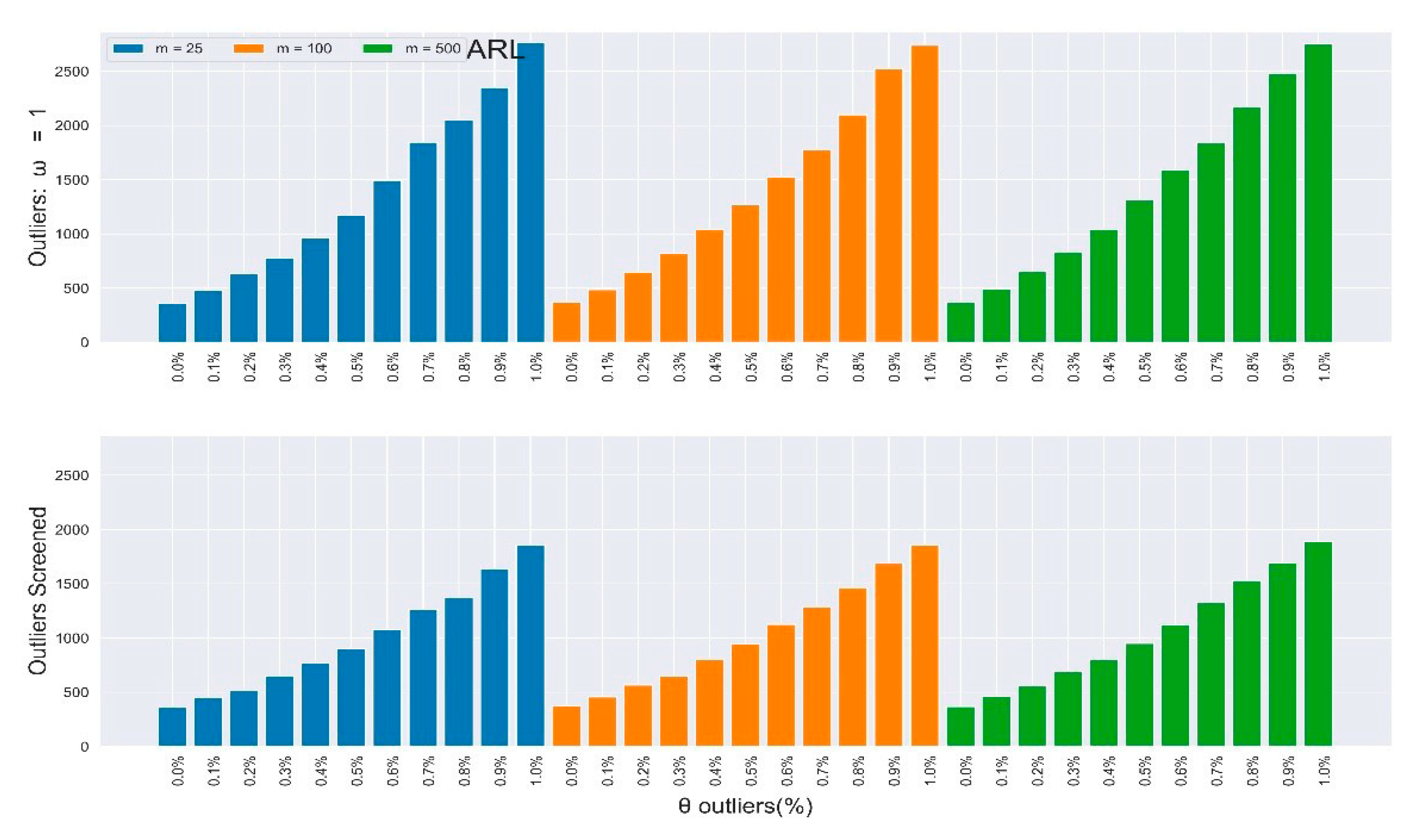
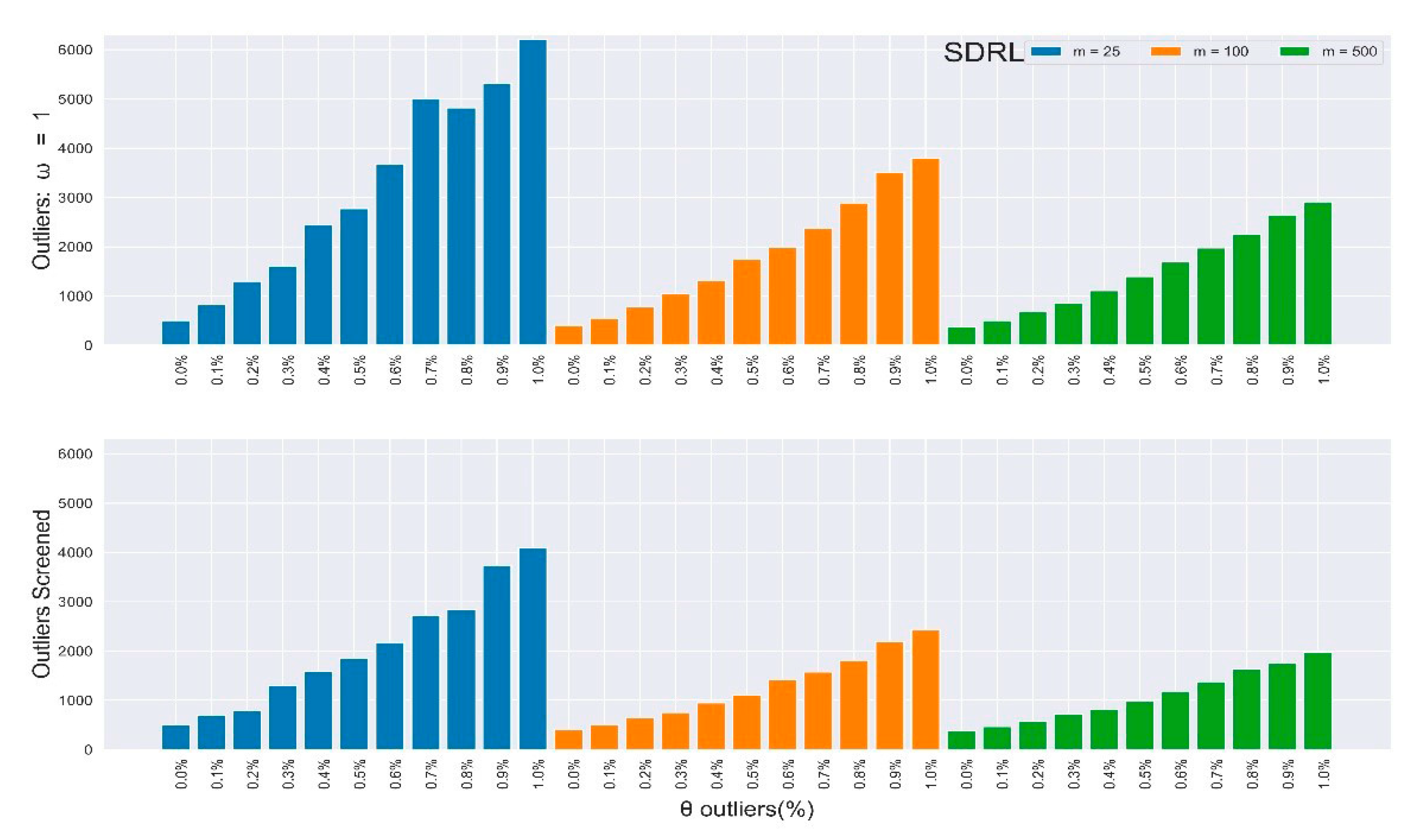
Furthermore, the rate of improvements appreciated as the percentage and magnitude of outliers increased. Figure 2, Figure 3, Figure 4 and Figure 5 depict the results in Table 3 and Table 4 (outliers without screening) side-by-side with Table 5 and Table 6 (SDRE outliers screening) to closely observe the improvements. Table 3 and Table 4 depict the IC and of the multivariate Shewhart chart from the mixed distribution in (5), with some percentages of outliers, and the magnitude . Here, all values should approximate to the nominal ARL of 370, since the environment was IC. When , it implies the absence of outliers in the process, so the ARL values for all the different m samples clustered around 370, although their SDRL values did not. It can be easily observed from the two tables that the outliers’ effect on the chart worsened as the percentage and magnitude of the outliers increased. Also, the effect on the ARL values was more obvious as the sample increased, and vice-versa for the SDRL values. In general, there was more than a 600% increment in the ARL and SDRL values when and a more than 3000% increment when . All of these were due to less than 10% outliers in the data.
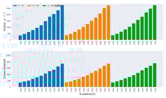
Figure 2.
In-control ARL values of the multivariate Shewhart chart from mixed distribution with and without SDRE multivariate outliers screening (ω = 1).

Figure 3.
In-control SDRL values of the multivariate Shewhart chart from a mixed distribution with and without SDRE multivariate outliers screening (ω = 1).
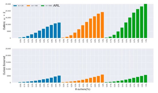
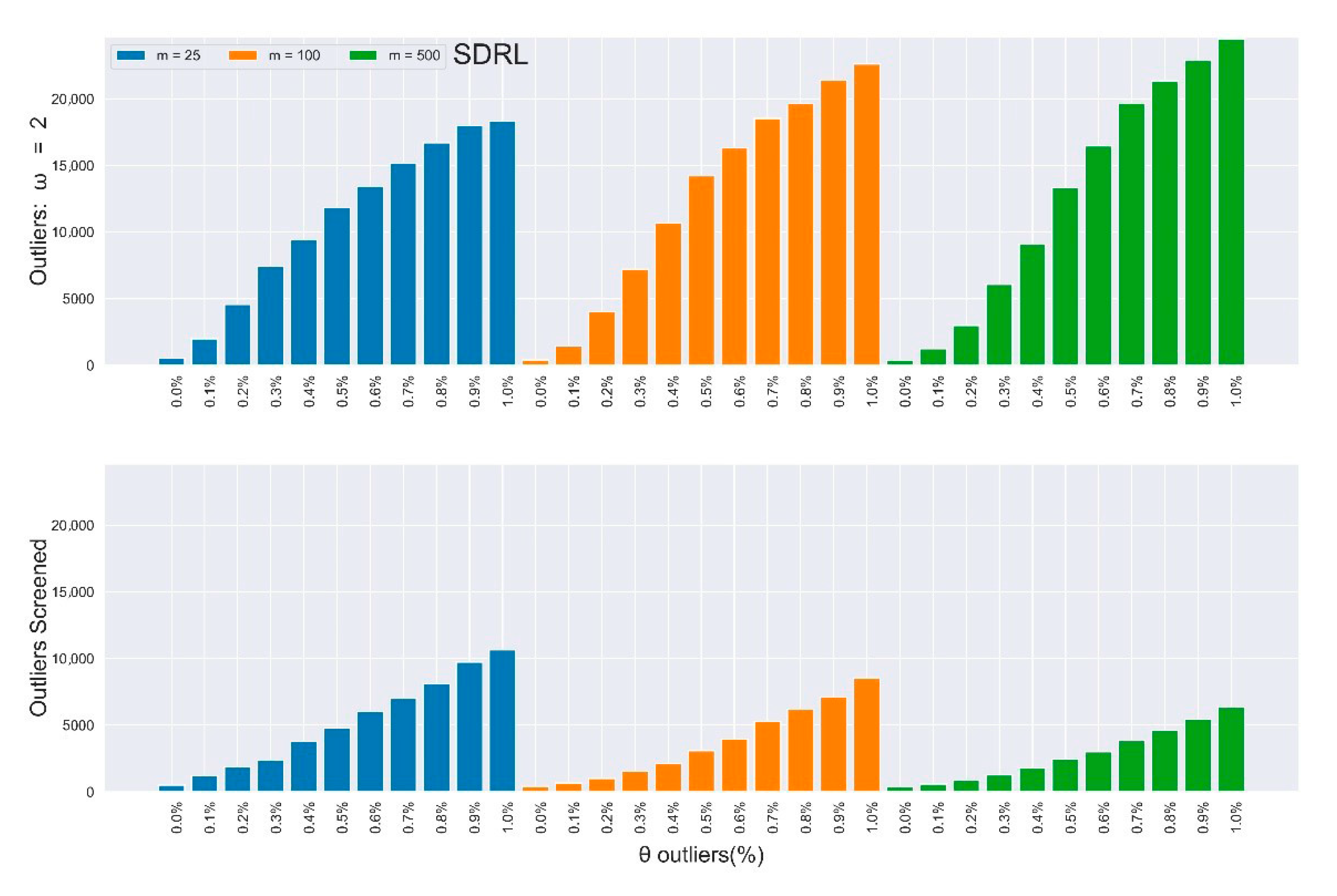
Figure 4.
In-control ARL values of the multivariate Shewhart chart from a mixed distribution with and without SDRE multivariate outliers screening (ω = 2).

Figure 5.
In-control SDRL values of the multivariate Shewhart chart from a mixed distribution with and without SDRE multivariate outliers screening (ω = 2).
The standard errors of the run length properties results reported in Table 1, Table 2, Table 3, Table 4, Table 5 and Table 6 were between 0.066% and 0.506%. These values validate the precision of the ARL and SDRL values. In addition, in Table 1 and Table 2, the results of the known cases are the best and the ideal results. However, the unknown case results improved and converged to those of the known cases as the phase-I sample increased. For the results of the outlier cases in Table 3, Table 4, Table 5 and Table 6, the outliers’ effect was more pronounced as the percentage, , and magnitude, , of outliers increased. These points further justify and validate the precision and consistency reported results.
4. Illustrative Example with Real-Life Dataset
In the manufacturing industry, carbon fiber tubes are a crucial and widely used material in numerous applications. They are preferred over many traditional materials such as aluminum, titanium, and steel, because of their unique features: resistance to fatigue, high strength and fitness to weight, resistance to corrosion, dimensional stability, and many more. This has resulted in carbon fiber gaining vast application in the manufacturing industry. The manufacturing process of carbon fibers is partly chemical and mechanical. They are mostly made of carbon atoms which bound together in microscopic crystals. The manufacturing process goes through spinning, stabilizing, carbonizing, surface treating, and sizing. The tubes are thin strands of material which are long in diameter. The minute size of carbon fibers requires close monitoring of the manufacturing process. In this study, we monitored three quality characteristics in the manufacturing process of a specific carbon fiber tubing. The characteristics are the inner diameter, thickness, and length of the tubes in inches.
The data were of two stages: in phase-I, each quality characteristic consisted of sample points each with a size of . Phase-II consisted of 20 observations each of size for every quality characteristic. Without any loss of generality, and for conformity with the aim of the study, the illustrative example was categorized into three cases:
- Case 1-Parameter estimation: Here, we employed the phase-I data to compute the default mean vector and covariance matrix ( and S), assuming the process parameters were unknown, and then used the estimates to compute the plotting statistics for monitoring the phase-II data as explained in (3) and plotted it against the UCL.
- Case 2-Parameter estimation with outliers: We infused θ = 7% of outliers with a magnitude ω = 3 and degrees of freedom v = 5 in the phase-I data, to simulate the mixed distribution described in (5), obtained the default parameter estimates ( and S), and then used the estimates to compute the plotting statistics for monitoring the phase-II dataset and plotted it against the UCL.
- Case 3-Parameter estimation with outliers and screening: The third case was similar to the second case, but we used the SDRE (t,V) as in (6) to estimate the process parameters from 25 phase-I samples, and to employ the SDRE in the Mahalanobis distance to detect and screen out the outliers. Then, we computed the default parameter estimates ( and S) from the remaining screened data, and then computed the plotting for monitoring the phase-II dataset and plotted it against the same UCL.
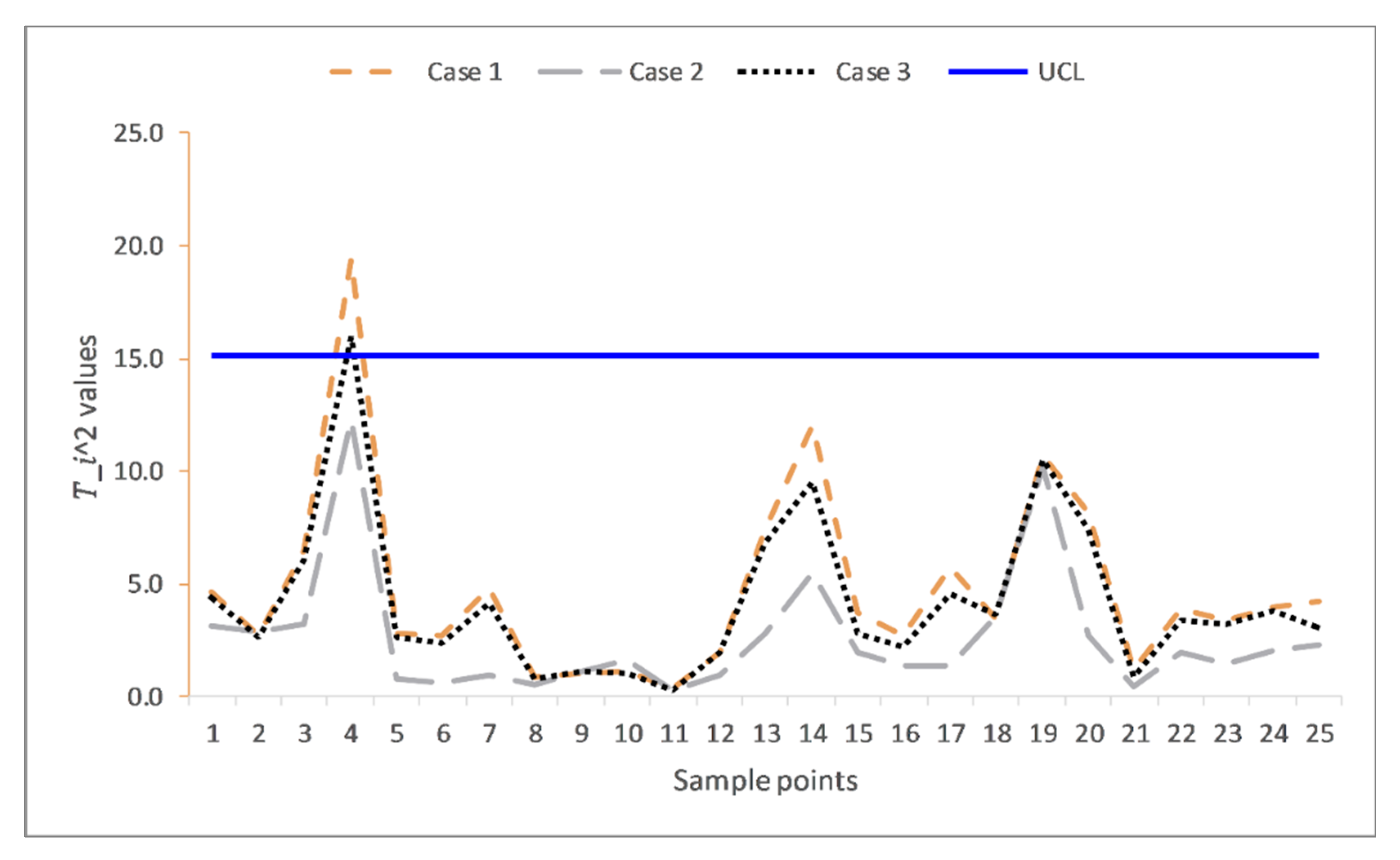
The summaries of the estimations of the parameters for these three cases are given in Table 7, while their plotting statistics and corresponding decisions are given in Table 8. In case 1, all observations are IC as they are all below the UCL = 15.16, except the fourth observation 19.4183, which plots beyond the UCL. This case represents when the process parameters are estimated from some preliminary samples without outliers. For case 2, all the plotting s were below the control limit despite the presence of outliers. The fourth observation that was plotted beyond the UCL in case 1 was masked due to the outliers’ effect. Case 2 reveals the effect of outliers in the preliminary samples. It also shows the inferiority of using the default mean vector and covariance matrix for estimating parameters, especially when the samples are prone to outliers. In case 3, the OoC fourth observation in case 1 is was detected OoC in this case. With the same magnitude and percentage of outliers as in case 2, case 3 was as efficient as case 1 when there were no outliers. This substantiates the improvement of the proposed SDRE and Mahalanobis distance’s procedures of estimating parameters and detecting outliers as claimed by the simulation results. Figure 6 depicts a visual representation of Table 8.
Table 7.
and S estimates from the phase-I sample for the three cases under study.
Table 8.
values and decisions of the three cases with θ = 0.07, ω = 3, and v = 5.
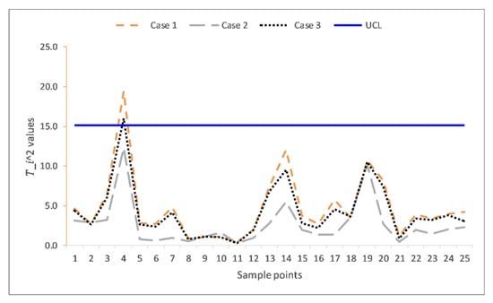
Figure 6.
The multivariate Shewhart charts from real life data extracted from carbon fiber tubes.
5. Conclusions
This research paper evaluated the in-control performance of the multivariate Shewhart control chart when the parameters were estimated from phase-I samples that were prone to outliers. The study observed the negative effect of estimation and outliers on the chart’s performance. Hence, we proposed a more efficient and robust multivariate Shewhart chart based on the Stahel-Donoho robust estimators and Mahalanobis distance to detect and screen outliers from the phase-I samples. Through the Monte-Carlo simulation approach, the ARL and SDRL for a different number of phase-I samples from small to medium to large were computed. The findings show that with the presence of outliers, even with large phase-I samples, the effect on the chart’s performance was severe. The results further show that the proposed chart based on SDRE and Mahalanobis distance restored the efficiency of the multivariate Shewhart chart with smaller phase-I samples. Therefore, it is rational to incorporate the SDRE and Mahalanobis distance in default multivariate Shewhart structures, especially when the process parameters are estimated from phase-I samples prone to outliers. The findings of this study were substantiated with real-life application in the manufacturing industry, where three qualities of carbon fiber tubes were monitored. The scope of this study was limited to monitoring the location parameter in a multivariate Shewhart chart. However, the study can be extended to monitoring dispersion parameters in multivariate Shewhart charts and other charting schemes, such as multivariate cumulative sum (MCUSM) and exponentially weighted moving average (MEWMA).
Author Contributions
Conceptualization, I.A.R. and N.A.; methodology, I.A.R., N.A. and M.R.; software, I.A.R. and M.R.A.; validation, N.A. and M.R.; formal analysis, I.A.R., N.A., M.R.A. and M.R.; investigation, I.A.R. and N.A.; resources, I.A.R.; data curation, I.A.R. and N.A.; writing—original draft preparation, I.A.R.; writing—review and editing, I.A.R., N.A., M.R.A. and M.R.; visualization, N.A., M.R.A. and M.R.; supervision, N.A., M.R.A. and M.R.; project administration, N.A. and M.R.; funding acquisition, N.A. and M.R. All authors have read and agreed to the published version of the manuscript.
Funding
This work was supported by the Deanship of Scientific Research (DRS) at King Fahd University of Petroleum and Minerals (KFUPM) under Project No. SB191047.
Institutional Review Board Statement
Not applicable.
Informed Consent Statement
Not applicable.
Data Availability Statement
The simulated data used in this article may be generated in R, using parameter values and the algorithm in Section 2.5. The real data set is available from the book referenced in [2].
Conflicts of Interest
The authors declare no conflict of interest.
References
- Hawkins, D.M. Identification of Outliers; Chapman and Hall: London, UK, 1980. [Google Scholar] [CrossRef]
- Montgomery, D.C. Introduction to Statistical Quality Control, 6th ed.; John Wiley & Sons, Inc.: New York, NY, USA, 2009. [Google Scholar]
- Psarakis, S.; Vyniou, A.K.; Castagliola, P. Some recent developments on the effects of parameter estimation on control charts. Qual. Reliab. Eng. Int. 2014, 30, 1113–1129. [Google Scholar] [CrossRef]
- Saleh, N.A.; Mahmoud, M.A.; Jones-Farmer, L.A.; Zwetsloot, I.; Woodall, W.H. Another look at the ewma control chart with estimated parameters. J. Qual. Technol. 2015, 47, 363–382. [Google Scholar] [CrossRef]
- Jones, L.A. The statistical design of ewma control charts with estimated parameters. J. Qual. Technol. 2018, 34, 277–288. [Google Scholar] [CrossRef]
- Abbas, N.; Abujiya, M.R.; Riaz, M.; Mahmood, T. Cumulative sum chart modeled under the presence of outliers. Mathematics 2020, 8, 269. [Google Scholar] [CrossRef] [Green Version]
- Raji, I.A.; Lee, M.H.; Riaz, M.; Abujiya, M.R.; Abbas, N. Outliers detection models in shewhart control charts; An application in photolithography: A semiconductor manufacturing industry. Mathematics 2020, 8, 857. [Google Scholar] [CrossRef]
- Abbas, N. A robust S2 control chart with Tukey’s and MAD outlier detectors. Qual. Reliab. Eng. Int. 2020, 36, 403–413. [Google Scholar] [CrossRef]
- Guarnieri, J.P.; Souza, A.M.; Jacobi, L.F.; Reichert, B.; da Veiga, C.P. Control chart based on residues: Is a good methodology to detect outliers? J. Ind. Eng. Int. 2019, 15, 119–130. [Google Scholar] [CrossRef] [Green Version]
- Bakar, Z.A.; Mohemad, R.; Ahmad, A.; Deris, M.M. A comparative study for outlier detection techniques in data mining. In Proceedings of the 2006 IEEE Conference on Cybernetics and Intelligent Systems, Bangkok, Thailand, 7–9 June 2006. [Google Scholar]
- Vidmar, G.; Blagus, R. Outlier detection for healthcare quality monitoring-A comparison of four approaches to over-dispersed proportions. In Quality and Reliability Engineering International; John Wiley and Sons Ltd.: Hoboken, NJ, USA, 2014; Volume 30, pp. 347–362. [Google Scholar]
- Zhang, H.; Albin, S. Detecting outliers in complex profiles using a χ2 control chart method. IIE Trans. (Inst. Ind. Eng.) 2009, 41, 335–345. [Google Scholar] [CrossRef]
- Manenti, F.; Buzzi-Ferraris, G. Criteria for outliers detection in nonlinear regression problems. Comput. Aided Chem. Eng. 2009, 26, 913–917. [Google Scholar] [CrossRef]
- Militino, A.F.; Palacios, M.B.; Ugarte, M.D. Outliers detection in multivariate spatial linear models. J. Stat. Plan. Inference 2006, 136, 125–146. [Google Scholar] [CrossRef]
- Fan, S.-K.S.; Huang, H.-K.; Chang, Y.-J. Robust multivariate control chart for outlier detection using hierarchical cluster tree in SW2. Qual. Reliab. Eng. Int. 2013, 29, 971–985. [Google Scholar] [CrossRef]
- Gnanadesikan, R.; Kettenring, J.R. Robust estimates, residuals, and outlier detection with multiresponse data. Biometrics 1972, 28, 81. [Google Scholar] [CrossRef]
- Pranata, A.; Sadik, K. Comparison of Hotelling, MVE and WD for Detecting Outlier in Robust Multivariate Control Chart. Int. J. Sci. Eng. Res. 2016, 7, 1138–1142. [Google Scholar]
- Hubert, M.; Debruyne, M.; Rousseeuw, P.J. Minimum covariance determinant and extensions. Wiley Interdiscip. Rev. Comput. Stat. 2018, 10, e1421. [Google Scholar] [CrossRef] [Green Version]
- Stahel, W.A. Breakdown of Covariance Estimators; Eidgenössische Technische Hochschule: Zürich, Switzerland, 1981. [Google Scholar]
- Maronna, R.A.; Yohai, V.J. The behavior of the Stahel-Donoho robust multivariate estimator. J. Am. Stat. Assoc. 1995, 90, 330–341. [Google Scholar] [CrossRef]
- Rousseeuw, P.; Hubert, M. High-breakdown estimators of multivariate location and scatter. In Robustness and Complex Data Structures: Festschrift in Honour of Ursula Gather; Springer: Berlin/Heidelberg, Germany, 2013; pp. 49–66. ISBN 9783642354946. [Google Scholar]
- Donoho, D.L. Breakdown Properties of Multivariate Location Estimator; Harvard University: Cambridge, MA, USA, 1982. [Google Scholar]
- Ghorbani, H. Mahalanobis distance and its application for detecting multivariate outliers. Math. Inf. 2019, 34, 583–595. [Google Scholar] [CrossRef]
- Zuo, Y.; Cui, H.; He, X. On the Stahel-Donoho estimator and depth-weighted means of multivariate data. Ann. Stat. 2004, 32, 167–188. [Google Scholar] [CrossRef]
- Abid, M.; Nazir, H.Z.; Riaz, M.; Lin, Z. In-control robustness comparison of different control charts. Trans. Inst. Meas. Control 2017, 40, 3860–3871. [Google Scholar] [CrossRef]
- Abid, M.; Nazir, H.Z.; Tahir, M.; Riaz, M.; Abbas, T. A Comparative Analysis of Robust Dispersion Control Charts with Application Related to Health Care Data. J. Test. Eval. 2019, 48, 247–259. [Google Scholar] [CrossRef]
- Zwetsloot, I.M.; Schoonhoven, M.; Does, R.J.M.M. Robust point location estimators for the EWMA control chart. Qual. Technol. Quant. Manag. 2016, 13, 29–38. [Google Scholar] [CrossRef] [Green Version]


Publisher’s Note: MDPI stays neutral with regard to jurisdictional claims in published maps and institutional affiliations. |
© 2021 by the authors. Licensee MDPI, Basel, Switzerland. This article is an open access article distributed under the terms and conditions of the Creative Commons Attribution (CC BY) license (https://creativecommons.org/licenses/by/4.0/).