Abstract
Today, generation and transmission expansion planning (G&TEP) to meet potential load growth is restricted by reliability constraints and the presence of uncertainties. This study proposes the reliability constrained planning method for integrated renewable energy sources and transmission expansion considering fault current limiter (FCL) placement and sizing and N-1 security. Moreover, an approach for dealing with uncertain events is adopted. The proposed planning model translates into a mixed-integer non-linear programming model, which is complex and not easy to solve. The problem was formulated as a tri-level problem, and a hybridization framework between meta-heuristic and mathematical optimization algorithms was introduced to avoid linearization errors and simplify the solution. For this reason, three meta-heuristic techniques were tested. The proposed methodology was conducted on the Egyptian West Delta system. The numerical results demonstrated the efficiency of integrating G&TEP and FCL allocation issues in improving power system reliability. Furthermore, the effectiveness of the hybridization algorithm in solving the suggested problem was validated by comparison with other optimization algorithms.
1. Introduction
The generation and transmission expansion planning (G&TEP) problem is one of the most debated topics within academia and decision-makers in the energy sector. G&TEP is concerned with identifying an optimum strategy for where, when, and how many generation and transmission facilities must meet the load growth while preserving the power system’s reliability and security performance [1,2].
G&TEP tasks are typically conducted individually rather than in an integrated way. Separated generation and transmission expansion planning exercises rarely lead to optimal overall planning and operating costs [1,2,3,4]. Various constraints have been suggested in the literature to shape more realistic G&TEP models [4]. The presented methodologies to handle the G&TEP problem can be grouped into four categories: (1) direct solution methods, (2) static or dynamic planning, (3) solution methods with uncertainties involved in the problem, and (4) solution methods with reliability engaged in the problem.
Solving the G&TEP optimization problem is an arduous task because the workable search space in G&TEP is typically ample, non-convex, and challenging to explore. The literature on this topic includes a variety of methods to solve it, which can be organized into three classes: (1) mathematical methods, (2) heuristic methods, and (3) meta-heuristic methods. Each method has its advantages and disadvantages [2,3]. The G&TEP model can be static or dynamic. The static model considers the demand for electrical power at the end of the planning horizon to find the location and number of new lines and generation stations. However, a dynamic model divides the planning horizon into many time intervals to solve the G&TEP problem.
The electrical system’s stochastic and reliability measurements impact the planning model’s efficiency and change the power system’s final configuration. Uncertain events, such as load demand variability and line contingencies, may occur. The installation of distributed generation (DG) units, such as renewable energy sources (RESs), poses new uncertainties [5,6]. These could dramatically affect the power system’s operation and weaken the grid’s reliability (for instance, a rolling blackout may occur, similar to the blackouts in California in 2020 [7]). Reliability measurements, such as N-1 security and short-circuit current (SCC) limits, are required to ensure that the generation and transmission facilities meet the future demand requirements during contingencies.
In the existing literature, while incorporating N-1 constraints into transmission expansion models is common practice, embedding conditions of SCCs into G&TEP models in the planning phase has been little discussed [8,9,10,11,12,13,14,15,16,17,18,19,20,21]. Ignoring SCC constraints may threaten the security of power grids because G&TEP reduces the equivalent network impedance, which, in turn, increases the short-circuit level of substations.
For instance, Sun et al. [8] introduced G&TEP models to handle power system uncertainties. They tested different clustering techniques to select suitable scenarios that represent uncertainties. Moghaddam [9] also proposed a G&TEP model that considers the impact of wind speed’s spatial distribution. A key limitation of Sun et al. [8] and Moghaddam [9] is that they did not address the N-1 security and SCC constraints. A G&TEP model, including energy storage systems, dynamic thermal rating systems, and optimal line switching, was proposed in other work [10]. Although the suggested algorithm presented a robust model to integrate RESs into power systems, reliability constraints were omitted. Zolfaghari et al. [11] proposed a bi-level multi-stage transmission expansion planning (TEP) considering wind investment. The market-clearing problem based on the AC-optimal power flow was planned, but the impact of reliability measurements on the suggested model was not discussed. Mazaheri et al. [12] integrated the TEP problem with energy storage system placement to deal with uncertainties. N-1 security was embedded in the proposed model, but the SCC constraint was not presented.
Moreover, Zhang et al. [13] suggested a planning model with compromised N-1 security, and Qorbani et al. [14] considered N-1 congestion and resilience constraints in the TEP model. However, both did not investigate the impact of power system uncertainties and SCC limits. A new expansion planning model of integrated electricity and gas networks with the high penetration of renewable energy resources was introduced in other work [15]. A scenario-based stochastic method was exploited to study the correlated uncertainty of photovoltaic generation and electrical loads; however, the SCC constraint was not included in the proposed model.
Regarding short-circuit level issues, Teimourzadeh et al. [16] and Wang et al. [17] introduced SCC limitations in the planning model. The suggested models depend on the location of new circuits to limit the SCC. This model is not helpful in some power systems, as we will see in this work. It is worth mentioning that the linear approximation, in [16,17], was necessary for the SCC analysis to tackle the non-linearity issues. Najjar et al. [18] suggested substituting new lines and opening the bus coupler of substations in a way that reduces SCC. The results showed that the first method cannot reduce the SCC below certain limits, but it is more beneficial than the second method for increasing wind farms integration.
Fault current limiters (FCLs) are special power system devices that minimize and reduce high SCCs to acceptable levels for the existing protection equipment, such as circuit breakers [19,20,21,22]. The FCL restricts the fault current to a predetermined level depending on the system configuration and the operating conditions. The power system planning considering FCL allocation was presented in other works [19,20,21]. These approaches were criticized because N-1 reliability and the impact of uncertainties were not embedded in the model. Furthermore, in [20,21], an equivalent linearized model was needed to handle the problem’s non-linearity. Therefore, a preventive mathematical approach to solving this problem is an imperative and critical task for the operators of the system.
The contributions of this paper are summarized as follows:
- The formulation and the presentation of a G&TEP stochastic model integrating allocation and the size of the FCLs are introduced to increase the penetration of RESs, meet reliability constraints and avoid rolling blackouts.
- To avoid linearization errors, a hybridization framework is suggested to solve the G&TEP problem and handle non-linear constraints.
- Three meta-heuristic techniques, namely lévy flight distribution (LFD), the sine cosine algorithm (SCA), and the success-history-based differential evolution with semi-parameter adaptation hybrid-covariance matrix adaptation evolution strategy algorithm (LSHADE-SPACMA), are employed to solve the problem, and the results obtained are analyzed and compared.
- The suggested methodology was conducted on the realistic transmission of the Egyptian West Delta Network (WDN) to validate the capability of the proposed algorithm.
The rest of this paper is organized as follows. Section 2 introduces the problem formulation, and Section 3 is devoted to the proposed model. The optimization techniques are shown in Section 4, while the results are presented and discussed in Section 5 and Section 6, respectively. Finally, the concluding remarks of this work are given in Section 7.
2. Problem Formulation
In this study, reliability constrained expansion planning problem is adopted that jointly resolves the problems of G&TEP and FCL allocation and considers the N-1 security and uncertainties. The proposed problem is formulated as a multi-objective optimization problem subjected to power flow and reliability constraints. The problem objective is to minimize the investment cost of installing new transmission lines, FCLs and generation units such that the operating cost, SCC, and the amount of load shedding (LS) are reduced. The uncertainties are modeled with a scenario-based approach. A set of scenarios representing the outcomes of RESs and demand variability are identified, then the problem is solved for each scenario in a cumulative process. To reduce the problem complexity, a scenario reduction technique is applied to decrease the number of considered scenarios.
2.1. The Mathematical Model
The DC power flow is commonly applied to formulate the model of G&TEP embedding SCC and N-1 constraints [16,17,18,19,20], and it was used in this work. The G&TEP model considering FCLs allocation and N-1 reliability is given as follows:
- Problem objective [16,17,18,19,20]:
- Constraints [16,17,18,19,20]:
During normal operation:
During abnormal operation:
- (1)
- Single-line outage:
- (2)
- Three-phase faults:
The objective function provided in (1) aims to reduce investment and operating costs and optimize the location of new transmission lines and generation units. Further, it determines the optimal place and size of the FCLs and the LS. and represent the investment costs in the TEP and GEP projects, respectively. Similarly, concerns the investment cost of installing FCL modules in existing and new circuits. is related to the operation cost of generation units. While includes the cost of LS to guarantee N-1 security.
Constraints (7) and (8) ensure that installed new circuits and renewable generation units are within their limits, and if they are constructed at scenario s, they will be available at subsequent scenarios. The active power balance at bus i and power flows through existing and new circuits are restricted by (9) and (10), respectively. The operation limits of generators limits and bus angles are enforced by (11)–(13). N-1 security constraints are dedicated in (14)–(16). The problem is solved for each single line outage, to calculate the amount of LS taking into account the power flow and generating constraints.
Constraint (17) allows placing FCLs modules in existing and newly constructed circuits and forces the installed modules at scenario S to be available in the following scenario. The SCC constraint is represented in (18). Because balanced three-phase faults are often the worst and are used to determine the circuit breaker capacity, it was considered in this work. For a balanced three-phase fault at bus i, the three-phase short-circuit current can be calculated by the following [16,17,18,19,20,21]:
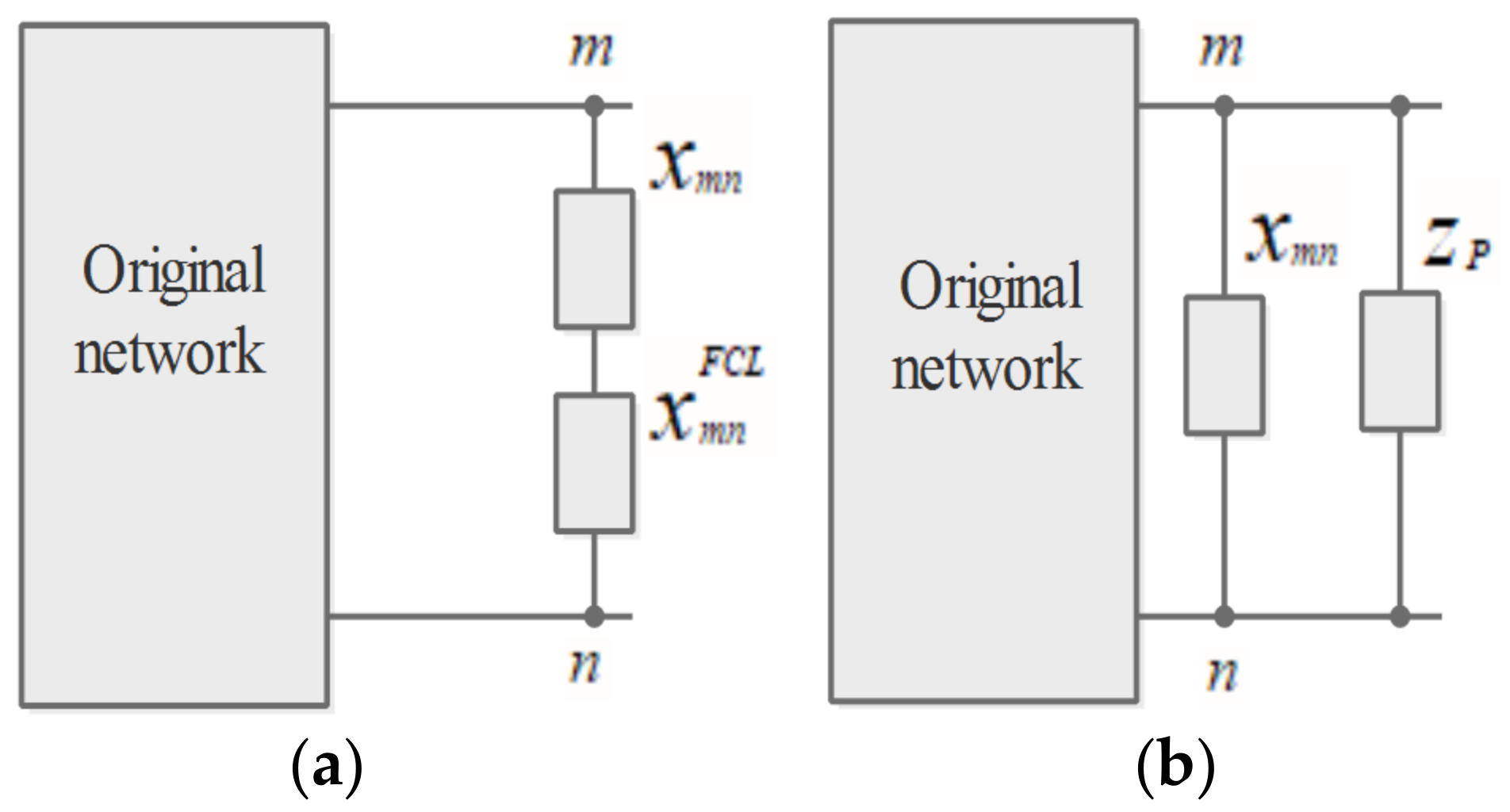
is the voltage before the fault at bus i. Commonly, can be set as 1.0 p.u. Zii is the Thevenin impedance seen from bus i. It is equivalent to the diagonal element of ZBus. Zii is changed as a result of adding a new circuit or FCL component. As shown in Figure 1, when FCL module with impedance is connected in series with a branch between bus m and n, is converted to a parallel impedance that equals [21]:
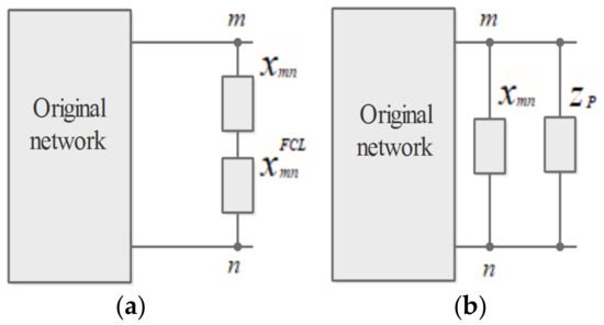
Figure 1.
Impact of adding FCL module to the network, (a) original network with added series FCL, (b) original network with equivalent impedance.
Therefore, change in due to adding a new circuit or FCL module is obtained by (21) and (22) [21].
In the above model, the constraints (19) and (21) are non-linear since impedances are variable due to adding new circuits and including FCLs. Several approaches have been reported in the literature to obtain a mixed-integer linear programming model; however, it may result in linearization errors. In this work, a hybridization framework between meta-heuristic and mathematical optimization algorithms was introduced to avoid linearization of non-linear constraints and simplify the solution. The problem is formulated as a tri-level optimization problem. The non-linear constraints are integrated into a single level, and a meta-heuristic technique is applied for solving this sub-problem. A meta-heuristic technique is selected because it is effective in dealing with non-linear models. The linear constraints are incorporated into the other levels, and two mathematical techniques are implemented to solve them. By applying this decomposition, the number of decision variables considered by the meta-heuristic algorithm is decreased, and therefore its performance is improved.
2.2. Uncertainty Modeling
One of the most practical approaches for modeling load and RES uncertainties is scenario-based techniques. The scenario analysis approach’s key concept is that several scenarios are created to present short-term and long-term load, wind speed, and solar radiation variations [8,23,24]. Then, the G&TEP problem is solved to determine the best solution for each scenario. One well-hedged answer is selected, which is the most suitable for all the designs.
In this work, a cumulative process was used. The problem was solved for each scenario based on the previous scenario results, as shown in Section 3. The applied approach ensures high robustness for all short-term and long-term uncertainties.
To create scenarios of load and RES variation, an approach to scenario generation and scenario reduction was adopted in [24,25]. The 1000 Monte-Carlo scenarios of each solar irradiance, wind speed, and load demand are incorporated to form a set of 1000 scenarios, with each design representing a vector of three elements (load demand, wind speed, and solar irradiance). The Monte- Carlo method relies on repeated random sampling and statistical analysis of simulation results. It starts with defining the probability density function (PDF) of uncertain variables. Then a pre-defined number of random samples are generated, and output values are calculated in a specific model. Load uncertainty is described using normal PDF [24,26]. While wind speed distribution is modeled using Weibull PDF, and solar irradiance is defined with the PDF of lognormal distribution [24,26]. This strategy is repeated several times until sufficient numbers of output variables are produced.
The 1000 scenarios are reduced to a representative set of 25 scenarios by applying the backward reduction technique of stochastic programming [25]. An increasing number of selected strategies might marginally improve the accuracy of the results; however, previous work [24] showed that optimization based on 25 scenarios is good.
3. Proposed Model
3.1. Proposed Hybridization Scheme
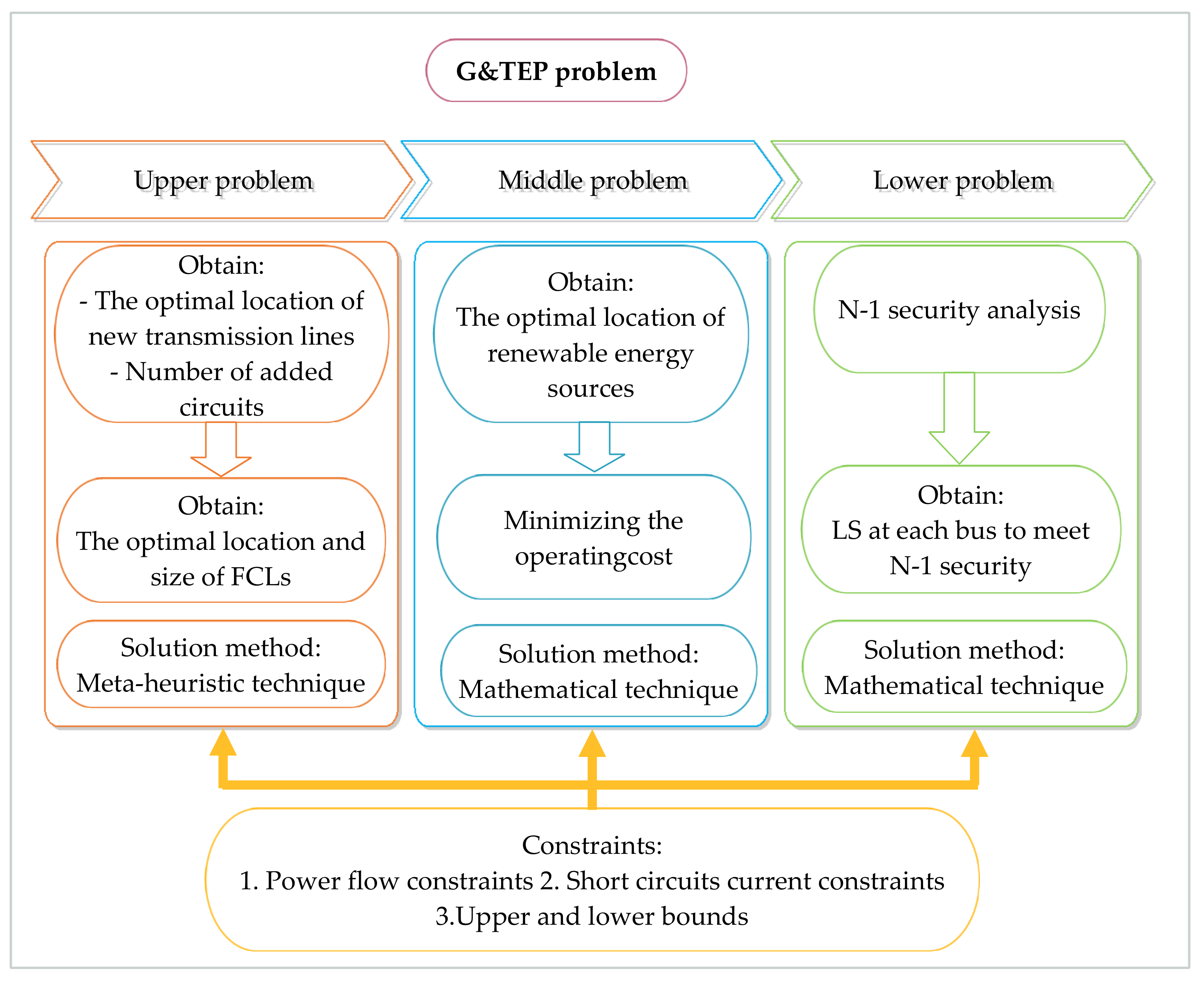
The suggested model is depicted in Figure 2. Optimization problems in (1)–(22) are incorporated into the tri-level formulation (upper-, middle-, and lower-level problems). The non-linear constraints are integrated into the upper-level problem, and a meta-heuristic technique is applied to make use of their ability to deal with non-linear systems. At the same time, the linear constraints are included in the middle and lower-level problems. By applying this decomposing, the last two levels are two simple optimization problems. Two mathematical techniques are employed to exploit their comparative advantages to reach optimal solutions within a few iterations.
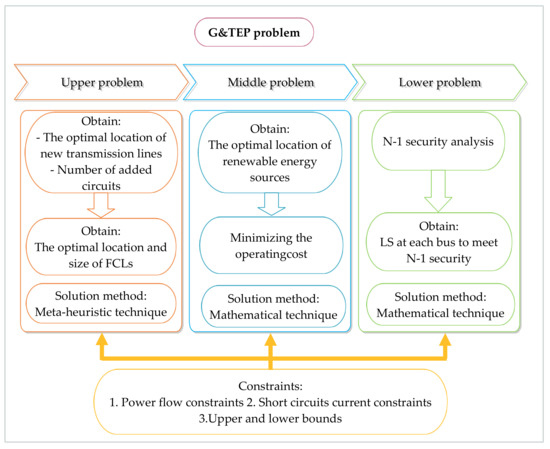
Figure 2.
Suggested model to solve the G&TEP problem.
3.1.1. Upper-Level Problem
The upper-level model can be planned as (7) and (17)–(23). The objective function provided in (23) aims to reduce the TEP project’s investment costs and determine the optimal place and size of the FCLs, considering the SCC limit and the constraints set out in (7) and (17)–(22). LFD, SCA, and LSHADE-SPACMA are examined to select the best one in solving this model.
3.1.2. Middle-Level Problem
The middle-level problem concerns the generators and operating constraints. The objectives function in (24) optimizes the location of the generation units and minimizes operating costs. Loads and DGs are considered uncertain parameters. The model of the middle-level is given by (8)–(13) and (24).
The above model is mixed-integer linear programming; therefore, branch-and-bound (B&B) method is applied to solve it.
3.1.3. Lower-Level Problem
The lower-level model seeks to find LS at each bus such that the reliability assessment (N-1 security) is validated and is represented by (14)–(16) and (25).This model is linear, and the interior-point (IP) method is employed to solve them. For each single branch outage,, the objective function in (25) is minimized in such a way that power flow and LS limit constraints (14)–(16) are confirmed. When the N-1 analysis is complete, the maximum LS at the bus (i) for all congestions is considered the final LS of bus i.
3.2. The Procedure of the Suggested Approach
The suggested algorithm for handling uncertainties and maintaining the reliability constraints is illustrated in Figure 3. It can be summarized in the following steps:
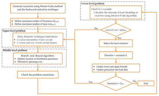
Figure 3.
Proposed flowchart of G&TEP.
- Step 1: Generate 1000 scenarios using the Monte-Carlo method to represent load, wind power source, and photovoltaic (PV) power source variation.
- Step 2: Select 25 scenarios using the backward reduction technique.
- Step 3: For each scenario, solve the upper level, medium level, and lower level of the G&TEP problem as follows:
- (a)
- Meta-heuristic optimization technique randomizes and to solve the upper-level problem.
- (b)
- After that, the medium-level problem is solved using the B & B algorithm to obtain DGs’ optimum location with minimum operating costs.
- (c)
- The IP method is applied to solve the lower problem to realize N-1 security.
- (d)
- If the candidate solution does not meet short-circuit and power flow constraints, it will be penalized by imposing high additional costs.
- (e)
- Do the iteration as shown in (a–d) until the iteration reaches the iteration limit.
- (f)
- Do the steps from (a–e) until the current run reaches the maximum number of runs.
- (g)
- Compare solutions of each run to select the optimal solution.
- (h)
- Go to the following scenario.
- Step 4: If the current scenario number is less than Smax, the lower bound of generation units, candidate routes, and FCL sizes are updated considering the system configuration under the previous scenario.
- Step 5: Repeat Steps 3 and 4 until Smax is reached.
4. Optimization Techniques
As mentioned earlier, SCA, LSHADE-SPACMA, and LFD are examined to solve the proposed problem. The three techniques are efficient in solving non-linear complex problems with a large feasible search space, and their features are summarized in Table 1. The operational mechanism of each algorithm is introduced in the following sub-sections.

Table 1.
Comparative analysis of SCA, LSHADE-SPACMA, and LFD.
4.1. Sine Cosine Algorithm
SCA is a meta-heuristic optimization algorithm that has been developed by Mirjalili et al. in 2016 [27]. SCA begins with some initial random candidate solutions. Based on sine and cosine functions, a mathematical model varies the candidate solution either outwards or towards the best solution. Due to the sine and cosine functions, this algorithm is called the sine cosine algorithm. Several random and adaptive variables are combined with this algorithm to emphasize exploring and exploiting the search space at various optimization milestones.
In SCA, the candidate solutions update their position as follows [27]:
where is the position of the current solution in i-th dimension at the t-th iteration, andis the position of the target point in the i-th dimension. R2, R3, and R4, are randomly selected, and R1 is adaptively changed as given in (28) [27]:
where T is the maximum number of iterations, and a is a constant.
R1, R2, R3, and R4 are the SCA’s main parameters, as seen in (26) and (27). R1 specifies the location that comes next. It may be in the region between the solution and destination or outside it. R2 sets the distance of the movement to or from the target position. R3 is a random weight to emphasize the target solution’s influence in determining the solution’s new location. Finally, R4 alternates between the cosine and sine components. Readers can refer to [27] for more details about the mechanism of operation.
4.2. LSHADE with Semi-Parameter Adaption Hybrid with CMA-ES
LSHADE-SPACMA was proposed by Mohamed et al. in 2017 [28]. It is a basis for hybridization between LSHADE-SPA and the updated version of CMA-ES. In LSHADE-SPA, a population of candidate solutions (decision vectors) is randomly generated within the upper and lower bounds. After that, a mutant vector corresponding to each population member, , is calculated in each iteration using the ‘current-to-pbest/1′ strategy as follows [28]:
The h-value here is supposed to be the control parameter for the mutation strategy’s greed to balance exploration and exploitation. Random indices (and were chosen from an external archive. For each generation, the target vector is combined with the mutated vector using the following equation to produce the trial vector,, based on the crossover rate, [28]:
is a uniformly distributed random number in the set [0, 1], and is a uniformly distributed random integer in the set [1, d] to ensure that at least one trial vector component is inherited from the mutant vector.
The control variables, F and , are adapted as proposed by Mohamed et al. [28]. When the current number of iterations is less than half of the maximum number of iterations, F and parameters are tuned using (31) and (32), respectively [28].
During the second half, the adaptation is concentrated on F, and the LSHADE adaptation is used to adapt the Fi parameter as follows [28]:
where and are a randomly selected memory slot where successful means of previous generations are stored. Memory index k was chosen randomly from the range [1, H], where H is the memory size, and is the standard deviation for the Cauchy distribution, which was set to 0.1.
The greedy selection technique is implemented for a minimization problem and is given by the following [28]:
Linear population size reduction (LPSR) is employed to boost the efficiency of LSHADE-SPA. The population size of the LPSR will be reduced by the linear function as follows [28]:
In CMA-ES, the search space is planned using a multivariate normal distribution. Gaussian distribution was applied to produce new individuals, which accounts for the population’s path over successive generations. The mean vector, covariance matrix, and step size are automatically adapted in CMA-ES.
A hybridization scheme between LSHADE-SPA and the modified CMA-ES version was implemented by Mohamed et al. in [28]. Each individual in the population produces an individual u offspring using either LSHADE-SPA or CMA-ES according to the probability variable (FCP) class. FCP values are chosen randomly from memory slots that are set to MFCP. One memory slot is modified at the end of each generation based on the output of each algorithm. As a result, populations were gradually assigned to a better performance algorithm. Updates were produced using individuals that successfully created new individuals. Readers can refer to [28] for more details about the LSHADE-SPACMA.
4.3. Lévy Flight Distribution
The LFD algorithm has been developed by Houssein et al. in 2020 [29]. Its main idea is based on the wireless sensor network environment associated with the motions of lévy flight (LF). The algorithm begins its mechanism by estimating the Euclidean distance (ED) for every two adjacent sensor nodes. Then the algorithm decides whether the sensor node will remain in its original location regarding the estimated distance, ED, or to shift it to another location. Another location will be executed using the LFs model, with the new position being in a location close to a sensor node with a low number of neighbors nodes or in a location where there are no sensor nodes in the deployment region (search space) to minimize the likelihood of overlapping among sensor nodes. It can be summarized as follows:
- Generate a population of candidate solutions.
- Define an upper bound (UB) and lower bound (LB) and a target solution.
- For each iteration, do the following:
- 1.
- For every two adjacent agents (main, neighbor), ED is calculated using the following (36):where and are the position coordinate of and , respectively.
- 2.
- If the ED is less than the threshold, the neighbor agent position is updated using (37) and (38). Based on a random value (R), if R is less than CSV, execute (37). If not, then run (38) to provide the algorithm with more chances to discover the search space.CSV is the scalar value that is compared with R in each update for the position. is the agent’s location with the fewest number of neighbors and is used as the LF direction. Lévy_ flight is a function that implements Lévy flight work in terms of step length and direction. It is implemented as follows:
- -
- Calculate the step length (leng) according to Mantegna’s algorithm.
- -
- Calculate the difference factor (DF) as follows:
- -
- Execute the actual random walk or flight with (40) such that is not outside the search space.
- 3.
- Update the main agent position using the following equation:So that:TP is the position of the best solution, and is the total target fitness of neighbors around . , and are random positive variables.
- 4.
- Bring the current agent back if it goes outside the boundaries, whether primary or neighbor.
- 5.
- Update the target solution.
More details about the LFD algorithm can be found in [29].
5. Numerical Results and Discussion
5.1. Selection of Suitable Optimization Technique
LSHADE-SPACMA, SCA, and LFD were tested to select the best technique to solve the G&TEP problem. For any meta-heuristic optimizer, there is no guarantee to state that the solution acquired is the optimal one, except that it is known. Therefore, in the Wilcoxon test [30], the standard deviation and number of scenarios in which the optimizer obtained the best solution were good indices for determining the efficient algorithm. The case studies were conducted in MATLAB r2017a on a DELL PC, with a model name of OptiPlex7050, including an Intel® Core™ i7′ CPU at 2.6 GHz and 16 GB RAM.
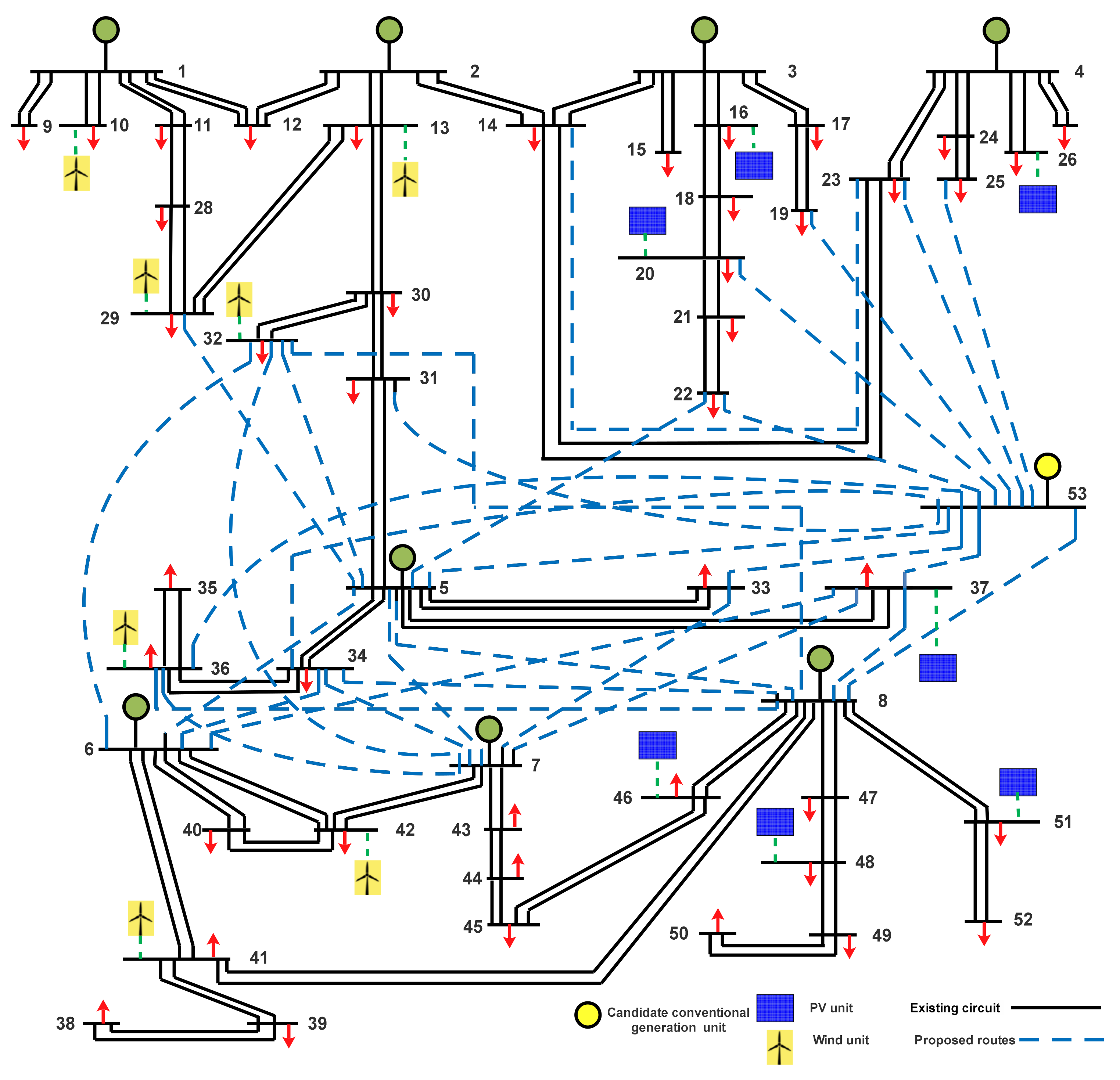
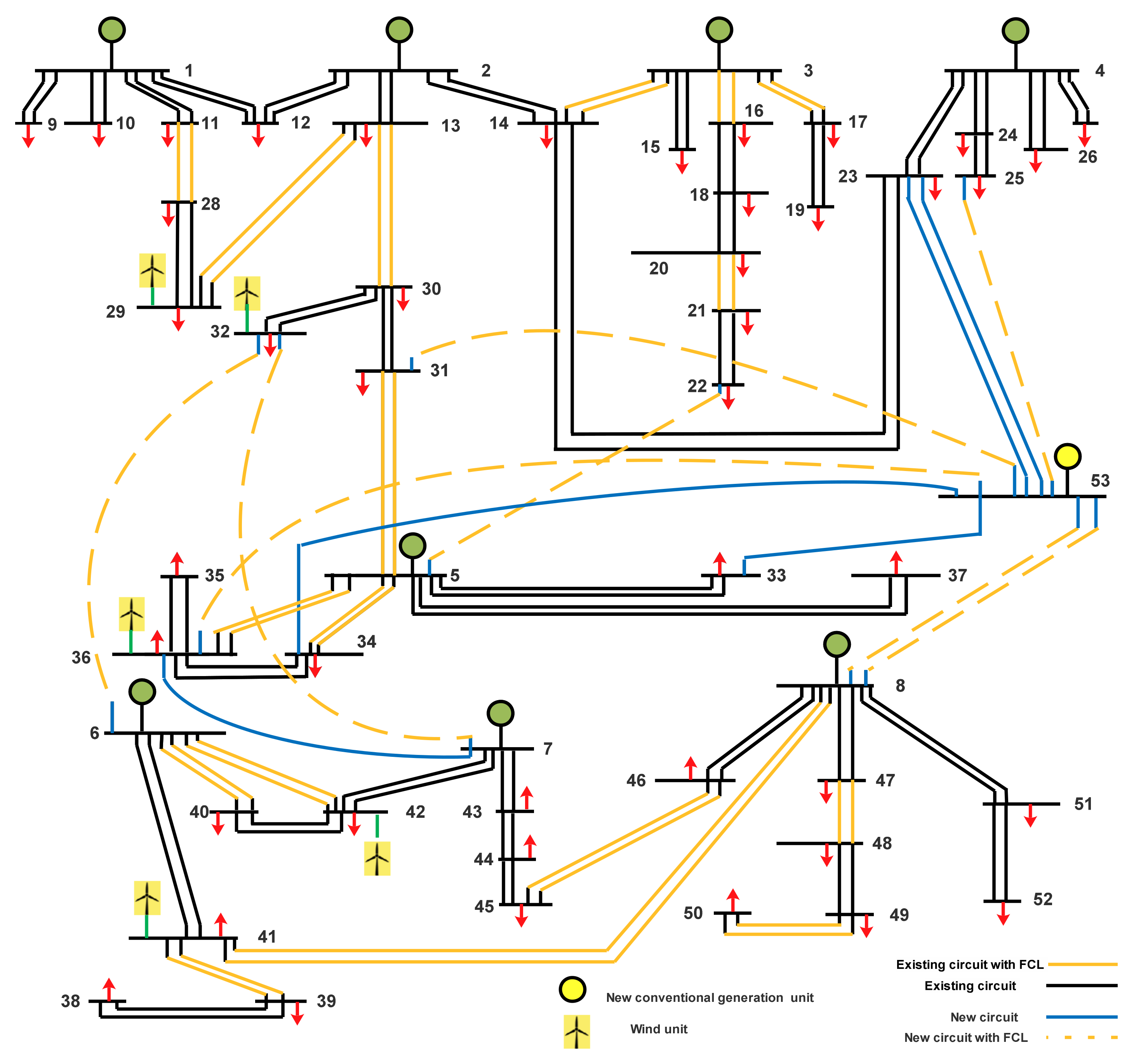
The three techniques were tested in WDN. The data of the system are introduced in other works [31]. To execute stochastic G&TEP, including RESs, the WDN configuration was modified as shown in Figure 4. The maximum capacity of the generation unit at bus 53 was decreased to 400 MW to create congestions. The candidate wind generation units were at buses 13, 10, 29, 32, 36, 41, and 42, and the PV units were at buses 16, 20, 26, 37, 46, 48, and 51. The total number of RESs should not have exceeded 6 units at the end of the planning period. Wind turbines and PV station data are introduced in other works [24,26]. The maximum capacity of wind and PV power plants is 100 MW. The investment and operation costs of generation units are listed in other work [32]. The cost of FCL is 0.51 million USD/ohm [33], and is 2 p.u.
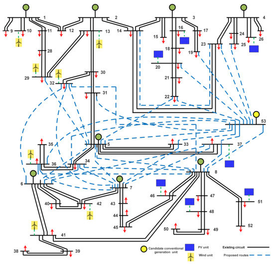
Figure 4.
Candidate generation units and transmission lines.
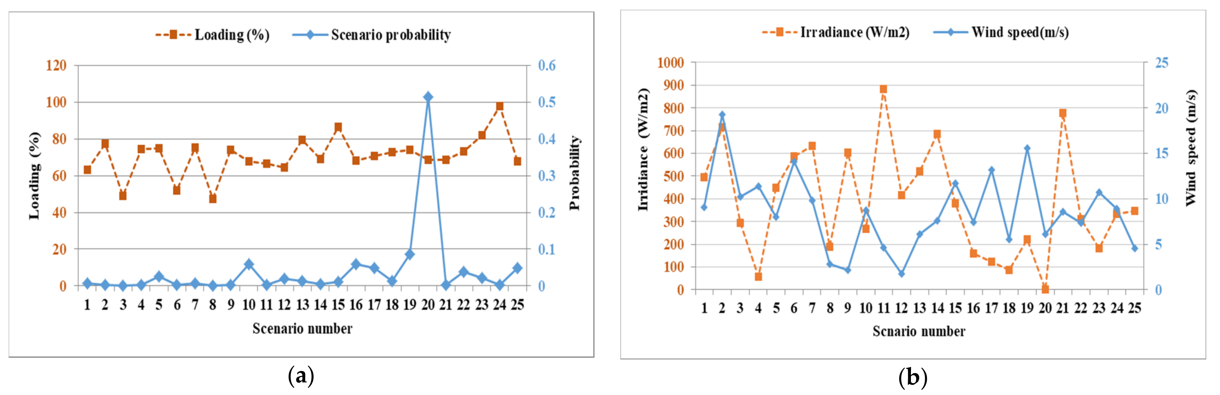
To calculate , a three-phase fault was performed at each bus for the initial configuration of the system in the year 2015, and the highest SCC was selected as a limit value of the system as a whole. The maximum limit of short-circuit current was 6.05 p.u. The selected scenarios using the backward reduction technique are depicted in Figure 5a,b. For each scenario, the upper-level and middle-level problems were solved, but the lower-level problem was ignored in this test because a complete N-1 analysis is too expensive for large systems. Therefore, it was only embedded in the model to obtain the final configuration of WDN. Due to such meta-heuristic-based algorithm randomness, the reported results were obtained over 30 independent runs and were compared to choose the best solution.
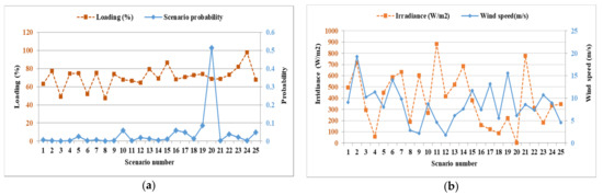
Figure 5.
Clustered scenarios: (a) loading percentages and probabilities, (b) wind speed and solar irradiances.
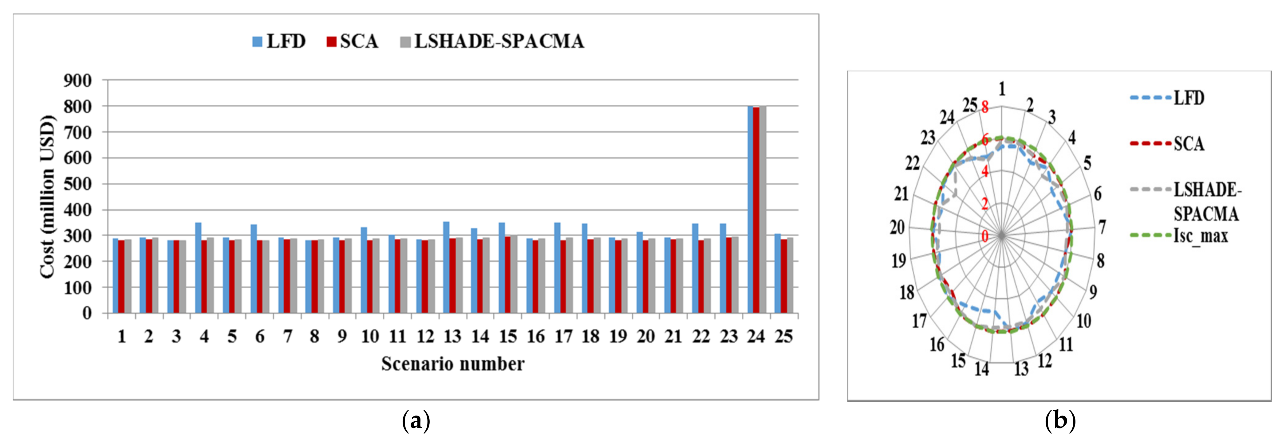
The efficiency of the three techniques for minimizing 117 variables is shown in Figure 6a,b. Figure 6a shows that SCA acquired the lowest investment cost in 24 scenarios, while the three techniques give the same results in Scenario Number 3. The SCCs for all scenarios do not exceed the maximum as seen in Figure 6b.

Figure 6.
Comparison between LFD, SCA, and LSHADE-SPACMA to solve the G&TEP problem: (a) the planning cost, (b) the contour of maximum short-circuits currents.
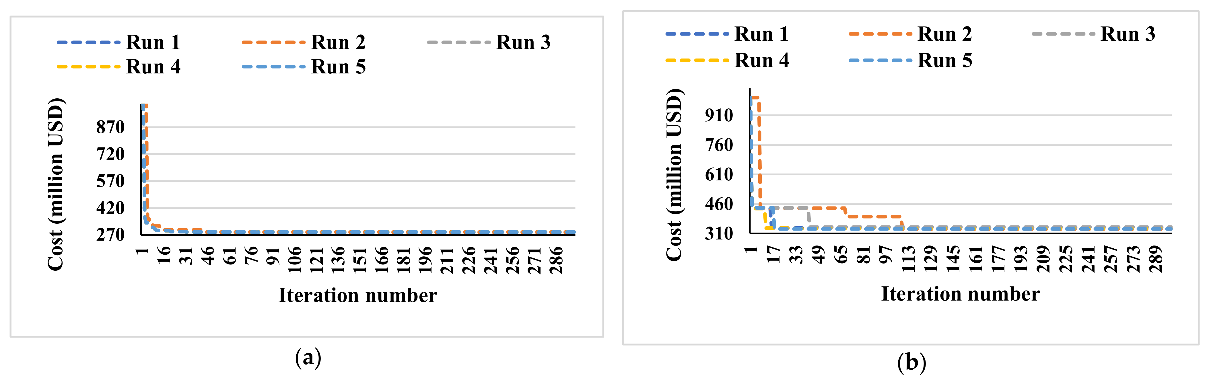
Table 2 contains the obtained results for p-values at 5% using the Wilcoxon test, standard deviation, and the time consumed to execute one run. The SCA clearly has a high-security response compared to the other techniques. The results showed SCA needed 327.089 s to implement one run. In contrast, LSHADE-SPACMA and LFD required 469.32 s and 353.231 s, respectively. Figure 7 shows the best five convergence rates for SCA and LFD (Scenario 25). Acceptable convergence curves of the SCA were achieved for finding the best solution that was better than LFD. The SCA provided very competitive performance and outperformed the other algorithms.
Table 2.
Convergence results of SCA, LSHADE-SPACMA, and LFD.
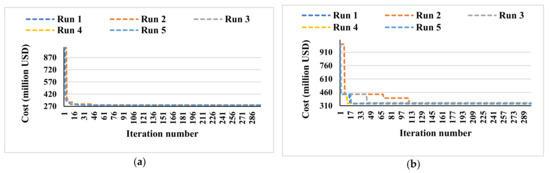
Figure 7.
Convergence curves of the best five runs for the SCA and LFD for Scenario Number 25: (a) SCA, (b) LFD.
5.2. WDN Planning
5.2.1. Robustness Measurement
To judge the applied approach’s efficiency, WDN was planned for Scenario Number 24 with and without embedding the system uncertainties in the G&TEP model and was compared with the WDN configuration using the suggested method. The WDN configuration for Scenario Number 24 was selected because it was the most critical scenario.
Each plan was tested for 1000 scenarios obtained using the Monte-Carlo method. is 3 p.u. Increasing led to more freedom to choose the location and the numbers of new circuits and RESs. The robustness index for each plan was calculated. The robustness index () is the ratio between the total scenarios that succeeded in meeting the power flow and short-circuit constraints to the total number of scenarios. The lower-level problem was not solved in this analysis.
WDN configurations under the three strategies are provided in Table 3, Table 4 and Table 5, respectively. The results showed that ignoring G&TEP uncertainties in G&TEP led to 96% robustness, and considering the critical scenario led to 99.8% robustness. However, the proposed approach led to 100% robustness. The results demonstrated the ability of the proposed approach to preventing possible blackouts.
Table 3.
Configuration of WDN for Scenario Number 24.
Table 4.
Configuration of WDN without considering uncertainties.
Table 5.
Configuration of WDN using the proposed approach without N-1 reliability.
5.2.2. Impact of Including FCL Allocation and Sizing in the G&TEP Problem
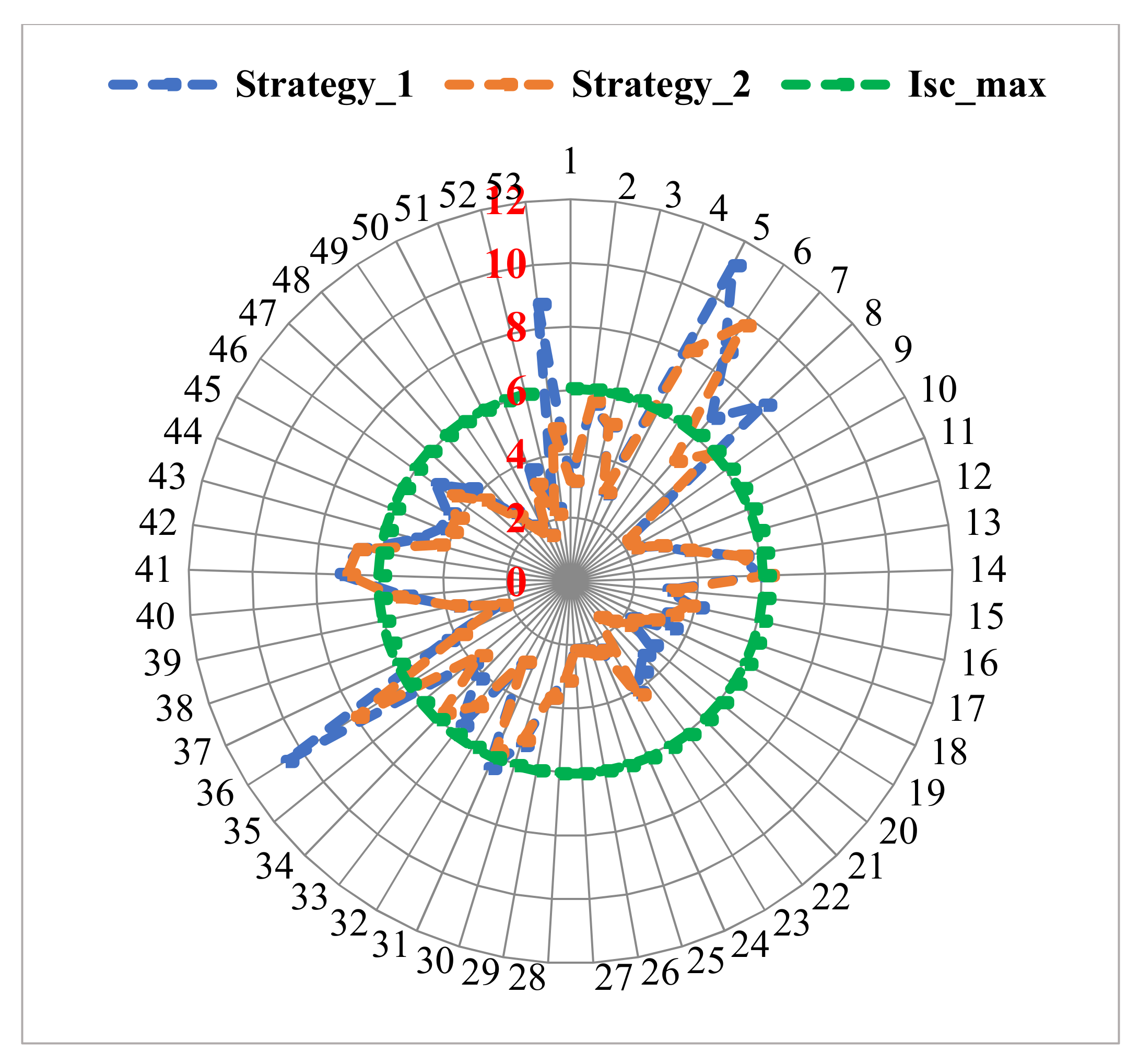
The impact of including FCL allocation and sizing in the G&TEP problem was studied, considering two strategies. The short-circuit penalty cost was 1000 million USD. In the first strategy, WDN was planned regarding the candidate routes and generation stations suggested in Fathy et al. [31]. The short-circuit current constraint was embedded in the model without using the FCLs introduced by Teimourzadeh et al. [16] and Wang et al. [17]. Figure 8 shows that the short-circuit currents at buses 5, 6, 7, 8, 31, 36, 41, 42, and 53 exceeded 6.05 p.u.
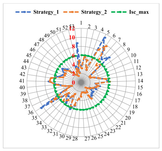
Figure 8.
The contour of short-circuit current at each bus without using FCLs.
In the second strategy, the system was planned considering the modification in Section 5.1. Similar to the first strategy, FCL allocation and sizing were not included in the problem. For Scenario Number 24, it was found that the short-circuit current at Buses 5, 6, 14, 36, 41, and 42 exceeded the maximum limit, as seen in Figure 8.
Both strategies demonstrated that the dependence on new circuit locations to mitigate the increase in short-circuit current is not useful in some power systems [34,35]. Hence, embedding FCLs during G&TEP is essential.
5.2.3. Configuration of WDN Considering N-1 Security
For N-1 security constraints, the three-level problems were solved. The final WDN configuration, considering uncertainties and the reliability constraints, is presented in Table 6, Figure 9 and Figure 10. Table 6 shows that 13 circuits, 42 FCLs, and 5 wind units were built at the end of the planning period.
Table 6.
Final configuration of WDN.

Figure 9.
Final configuration of the WDN.
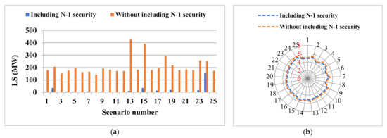
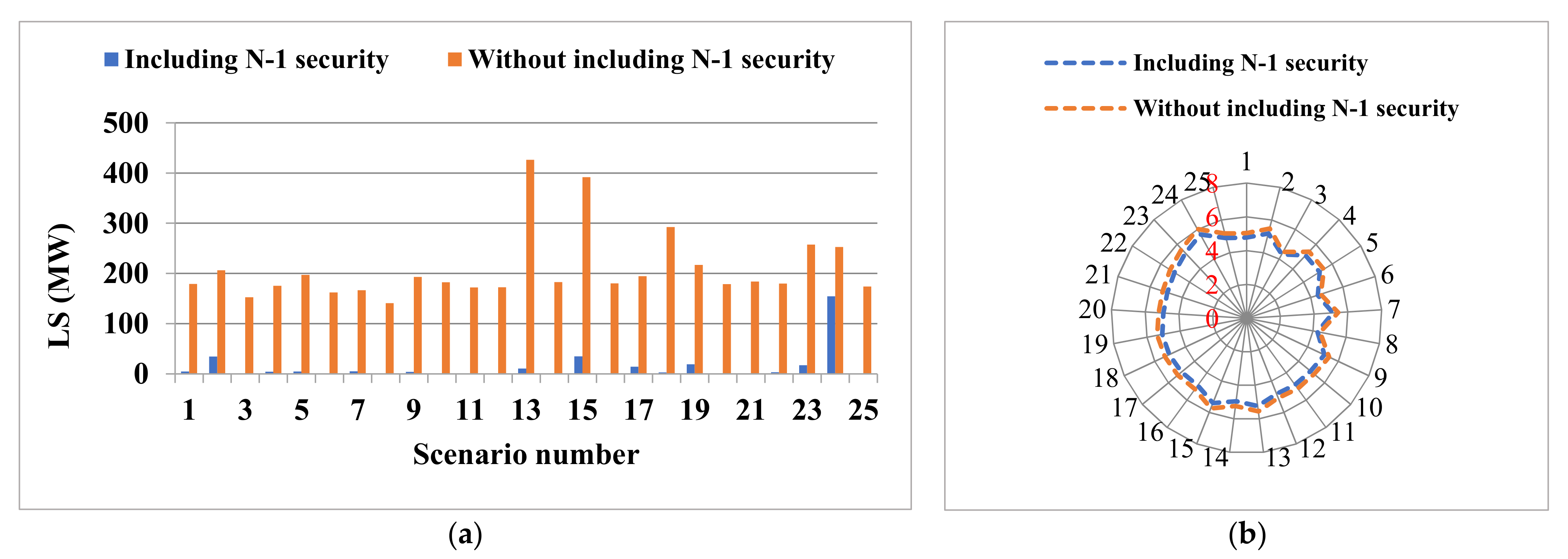
Figure 10.
WDN planning with/ without including N-1 security: (a) amount of LS for each scenario; (b) the contour of maximum short-circuits current for each scenario.
Figure 10a shows that including N-1 security in the planning model leads to a noticeable reduction in the level of LS for each scenario. The maximum LS was reduced from 426.28 MW to 154.35 MW. Besides, the numerical results demonstrated that integrating the load shedding problem with N-1 security analysis is essential for some power systems because the candidate transmission routes, and generation unit may not preserve the power system’s reliability and security performance during contingencies. Figure 10b depicts that the SCC did not exceed the maximum value, which refers to SCC constraints were achieved.
6. Discussion
In this work, a generation and transmission expansion plan for the WDN was proposed. The problem was formulated as a tri-level optimization problem, and the scenario-based technique was adopted to model the uncertainties. A hybridization approach between a meta-heuristic method and two mathematical techniques was applied for solving the problem. Three meta-heuristic techniques such as SCA, LFD, and LSHADE-SPACMA were tested and compared in terms of convergence speed and quality of the obtained solutions. The findings indicated that the SCA succeeded in finding a high-quality solution in 100% of test scenarios [36], whereas the success percentage of LSHADE-SPACMA and LFD was 4%. The results also showed the SCA reached the optimal solution faster than the LFD by 26.142 s and LSHADE-SPACMA by 142.231 s. The analysis and simulation demonstrated that the applied approach succeeded in solving the problem without implementing a linearization strategy as required in some works in the literature.
The results ensured that embedding FCL allocations and sizing problems in the G&TEP problem was necessary for the WDN. The reliance on new circuit locations, as suggested in some studies in the literature, to maintain the maximum short-circuit current within the permissible limit was not effective. The short-circuit current without FCLs exceeded 11.5 p.u at some buses (1.9 times the maximum permissible value).
The results showed that ignoring power system uncertainties or applying an ineffective algorithm to deal with uncertainties threatened the power system’s security and reliability. The network, when the uncertainties were neglected, was prone to a partial or complete blackout for 4% of the representative scenarios. The suggested cumulative process to deal with short-term and long-term uncertainties increased the robustness of the G&TEP model. It led to a more accurate and secure plan (100% security).
The results demonstrated that including N-1 security constraints in the G&TEP problem is indispensable to reduce the LS at each bus during contingencies and changes the overall system configuration. In addition, calculating the LS problem with N-1 security analysis is a prerequisite in some power systems because candidate transmission lines and generation units may not validate N-1 security without load shedding. Ignoring the N-1 security in the planning model caused an LS of 19.4%. Whilst this percentage was reduced to 7% when the N-1 constraint was considered.
Finally, separate dealing with G&TEP, FCL allocation and sizing, uncertainty handling, and power system reliability problems weaken the power system and always makes it exposed to rolling blackout.
7. Conclusions
A stochastic security-constrained G&TEP model was proposed in this paper. Three-level problems were solved to identify optimal locations for new routes and DGs and reduce operating costs when complying with N-1 security and short-circuit current constraints. In addition, an approach to deal with renewable source stochastic and load consumption variability was introduced. A meta-heuristic technique combined with two mathematical optimization techniques was applied to solve the G&TEP problem. LFD, SCA, and LSHADE-SPACMA were examined to minimize TEP cost and find locations and sizes for the FCLs. The B&B method was applied to minimize operating costs and to find optimal places for generation units. The IP method was used to obtain an amount of LS when N-1 security analysis was carried out. The findings of this study were quite promising, and thus the following conclusion can be drawn:
- The results showed that the SCA is superior to LFD and LSHADE-SPACMA in terms of convergence speed and reaching the global optimum. The calculation time of SCA was 327.089 s, while it was 469.32 s and 353.231 s for LSHADE-SPACMA and LFD, respectively. The SCA gave the best solutions in 24 tested scenarios, whereas the three techniques gave the same results in one scenario. Moreover, the SCA had the lowest standard deviation of 0.4872%.
- The results demonstrated that G&TEP correlated with FCL allocation is necessary for some power systems to meet SCC constraints, and the reliance on the new circuit locations is not useful in some power systems such as the WDN. It was found that the short-circuit current if FCLs were not used, was more than 11.5 p.u.
- The robustness of the adopted approach in handling uncertainties was demonstrated. It reached 100%.
- Integrating N-1 constraint with the G&TEP model improves power system reliability and decreases the amount of LS. The results indicated that the amount of LS for a single circuit outage increased from 154.35 MW to 426.28 MW when the N-1 security was ignored.
Author Contributions
M.M.R. and S.H.E.A.A. designed the problem under study; M.M.R. performed the simulations and obtained the results; S.H.E.A.A. analyzed the obtained results; M.M.R. wrote the paper, which was further reviewed by S.H.E.A.A., Y.A., Z.M.A., A.E.-S. and M.M.S. All authors have read and agreed to the published version of the manuscript.
Funding
This research received no external funding.
Institutional Review Board Statement
Not applicable.
Informed Consent Statement
Not applicable.
Data Availability Statement
The data presented in this study are available on request from the corresponding author. The data are not publicly available due to their large size.
Conflicts of Interest
The authors declare no conflict of interest.
Nomenclature
Input Data and Indices
| B&B | Branch-and-bound method |
| CMA-ES | Covariance matrix adaptation evolution strategy |
| DCPF | DC power flow |
| DG | Distributed generation |
| LS | load shedding (MW) |
| FCL | Fault current limiter |
| GEP | Generation expansion planning |
| G&TEP | Generation and transmission expansion planning |
| IP | Interior-point |
| LFD | Lévy flight distribution |
| LP | Linear programming |
| LPSR | Linear population size reduction |
| LSHADE-SPACMA | Linear population size reduction success history based differential evolution with semi-parameter adaptation hybrid with CMA-ES |
| MILP | Mixed-integer linear programming |
| PV | Photovoltaic |
| RESs | Renewable energy sources |
| SCA | Sine cosine algorithm |
| SPA | Semi-parameter adaptation |
| TEP | Transmission expansion planning |
| WDN | Egyptian West Delta network |
| N, S | Sets of buses and scenarios, respectively |
| Maximum number of scenarios | |
| Cost of the circuit between buses i and j | |
| The cost of installing an FCL between bus i and bus j | |
| Three-phase short-circuit current at bus i of scenario s and the maximum short-circuit current limit, respectively | |
| The load demand (MW) at bus i for scenario s | |
| Actual power generation for scenario s, the minimum capacity, and the maximum capacity of renewable energy source at bus i, respectively | |
| Actual power generation of conventional power plant for scenario s, the minimum capacity, and the maximum capacity of traditional power source at bus i, respectively | |
| Susceptance of route between buses i and j | |
| The maximum number of circuits, and the number of new circuits for scenario s between buses i and j, respectively | |
| Impedance of FCL between buses i and j | |
| The minimum and the maximum impedance of FCL between buses i and j | |
| Active power flow and the active power flow limit in the i-j right of way (MW), respectively | |
| Three-phase short-circuit current at bus i and the maximum short-circuit current limit, respectively | |
| Voltage angles at bus i | |
| The cost and location of installation of the new generation station at bus i | |
| The operation cost of generator i (US $/MWh). | |
| The cost and amount of LS at bus i, respectively | |
| Set of candidate solutions | |
| Upper bound and lower bound of the decision vector, respectively | |
| Mutant vector corresponding to each population member, | |
| F | Scale factor |
| CR | Crossover rate |
| Best individual vector with the best fitness value at t generation in the population |
References
- Naderi, E.; Pourakbari-kasmaei, M.; Lehtonen, M. Transmission expansion planning integrated with wind farms: A review, comparative study, and a novel profound search approach. Int. J. Electr. Power Energy Syst. 2020, 115, 105460. [Google Scholar] [CrossRef]
- Mahdavi, M.; Antunez, C.; Ajalli, M.; Romero, R. Transmission expansion planning: Literature review and classification. IEEE Syst. J. 2019, 13, 3129–3140. [Google Scholar] [CrossRef]
- Babatunde, O.; Munda, J.; Hamam, Y. A comprehensive state-of-the-art survey on power generation expansion planning with intermittent renewable energy source and energy storage. Int. J. Energy Res. 2019, 43, 6078–6107. [Google Scholar] [CrossRef]
- Gacitua, L.; Gallegos, P.; Henriquez-Auba, R.; Lorca, Á.; Negrete-Pincetic, M.; Olivares, D.; Valenzuela, A.; Wenzel, G. A comprehensive review on expansion planning: Models and tools for energy policy analysis. Renew. Sustain. Energy Rev. 2019, 98, 346–360. [Google Scholar] [CrossRef]
- Wang, Y.; Zhou, X.; Shi, Y.; Zheng, Z.; Zeng, Q.; Chen, L.; Xiang, B.; Huang, R. Transmission Network Expansion Planning Considering Wind Power and Load Uncertainties Based on Multi-Agent DDQN. Energies 2021, 14, 6073. [Google Scholar] [CrossRef]
- Cañas-Carretón, M.; Carrión, M.; Iov, F. Towards Renewable-Dominated Power Systems Considering Long-Term Uncertainties: Case Study of Las Palmas. Energies 2021, 14, 3317. [Google Scholar] [CrossRef]
- Rolling Blackouts in California Have Power Experts Stumped. Available online: https://www.nytimes.com/2020/08/16/business/california-blackouts.html (accessed on 20 June 2021).
- Sun, M.; Teng, F.; Konstantelos, I.; Strbac, G. An objective-based scenario selection method for transmission network expansion planning with multivariate stochasticity in load and renewable energy sources. Energy 2018, 145, 977–991. [Google Scholar] [CrossRef]
- Moghaddam, S.Z. Generation and transmission expansion planning with high penetration of wind farms considering spatial distribution of wind speed. Int. J. Electr. Power Energy Syst. 2019, 106, 232–241. [Google Scholar] [CrossRef]
- Dehghan, S.; Amjady, N.; Aristidou, P. A robust coordinated expansion planning model for wind farm-integrated power systems with flexibility sources using affine policies. IEEE Syst. J. 2020, 14, 4110–4118. [Google Scholar] [CrossRef]
- Zolfaghari, S.; Akbari, T. Bilevel transmission expansion planning using second-order cone programming considering wind investment. Energy 2018, 154, 455–465. [Google Scholar] [CrossRef]
- Mazaheri, H.; Abbaspour, A.; Fotuhi-Firuzabad, M.; Moeini-Aghtaie, M.; Farzin, H.; Wang, F.; Dehghanian, P. An online method for MILP co-planning model of large-scale transmission expansion planning and energy storage systems considering N-1 criterion. IET Gener. Transm. Distrib. 2021, 15, 664–677. [Google Scholar] [CrossRef]
- Zhang, H.; Vittal, V.; Heydt, G.T.; Quintero, J. A mixed-integer linear programming approach for multi-stage security-constrained transmission expansion planning. IEEE Trans. Power Syst. 2012, 27, 1125–1133. [Google Scholar] [CrossRef]
- Qorbani, M.; Amraee, T. Long term transmission expansion planning to improve power system resilience against cascading outages. Electr. Power Syst. Res. 2021, 192, 106972. [Google Scholar] [CrossRef]
- Yamchi, H.B.; Safari, A.; Guerrero, J.M. A multi-objective mixed integer linear programming model for integrated electricity-gas network expansion planning considering the impact of photovoltaic generation. Energy 2021, 222, 119933. [Google Scholar] [CrossRef]
- Teimourzadeh, S.; Aminifar, F. MILP formulation for transmission expansion planning with short-circuit level constraints. IEEE Trans. Power Syst. 2016, 31, 3109–3118. [Google Scholar] [CrossRef]
- Wang, J.; Zhong, H.; Xia, Q.; Kang, C. Transmission network expansion planning with embedded constraints of short circuit currents and N-1 security. J. Mod. Power Syst. Clean Energy 2015, 3, 312–320. [Google Scholar] [CrossRef] [Green Version]
- Najjar, M.; Falaghi, H. Wind-integrated simultaneous generation and transmission expansion planning considering short-circuit level constraint. IET Gener. Transm. Distrib. 2019, 13, 2808–2818. [Google Scholar] [CrossRef]
- Moon, G.; Lee, J.; Joo, S. Integrated generation capacity and transmission network expansion planning with superconducting fault current limiter (SFCL). IEEE Trans. Appl. Supercond. 2013, 23, 5000510. [Google Scholar] [CrossRef]
- Gharibpour, H.; Aminifar, F.; Bashi, M.H. Short-circuit-constrained transmission expansion planning with bus splitting flexibility. IET Gener. Transm. Distrib. 2018, 12, 217–226. [Google Scholar] [CrossRef]
- Esmaili, M.; Ghamsari-Yazdel, M.; Amjady, N.; Chung, C.Y.; Conejo, A.J. Transmission expansion planning including TCSCs and SFCLs: A MINLP approach. IEEE Trans. Power Syst. 2020, 35, 4396–4407. [Google Scholar] [CrossRef]
- Hamidi, M.; Chabanloo, R. Optimal allocation of distributed generation with optimal sizing of fault current limiter to reduce the impact on distribution networks using NSGA-II. IEEE Syst. J. 2019, 13, 1714–1724. [Google Scholar] [CrossRef]
- Khan, N.H.; Wang, Y.; Tian, D.; Jamal, R.; Ebeed, M.; Deng, Q. Fractional PSOGSA algorithm approach to solve optimal reactive power dispatch problems with uncertainty of renewable energy resources. IEEE Access 2020, 8, 215399–215413. [Google Scholar] [CrossRef]
- Biswas, P.; Suganthan, P.; Mallipeddi, R.; Amaratunga, G. Optimal reactive power dispatch with uncertainties in load demand and renewable energy sources adopting scenario-based approach. Appl. Soft Comput. 2019, 75, 616–632. [Google Scholar] [CrossRef]
- Growe-Kuska, N.; Heitsch, H.; Romisch, W. Scenario reduction and scenario tree construction for power management problems. In Proceedings of the 2003 IEEE Bologna Power Tech. Conference, Bologna, Italy, 23–26 June 2008. [Google Scholar]
- Chang, T. Investigation on frequency distribution of global radiation using different probability density functions. Int. J. Appl. Sci. Eng. 2010, 8, 99–107. [Google Scholar]
- Mirjalili, S. SCA: A sine cosine algorithm for solving optimization problems. Knowl.-Based Syst. 2016, 96, 120–133. [Google Scholar] [CrossRef]
- Mohamed, A.W.; Hadi, A.; Fattouh, A.; Jambi, K. LSHADE with semi-parameter adaptation hybrid with CMA-ES for solving CEC 2017 benchmark problems. In Proceedings of the 2017 IEEE Congress on Evolutionary Computation (CEC), San Sebastian, Spain, 5–8 June 2017; pp. 145–152. [Google Scholar]
- Houssein, E.H.; Saad, M.R.; Hashim, F.A.; Shaban, H.; Hassaballah, M. Lévy flight distribution: A new meta-heuristic algorithm for solving engineering optimization problems. Eng. Appl. Artif. Intell. 2020, 94, 103731. [Google Scholar] [CrossRef]
- Wilcoxon, F. Individual Comparisons by Ranking Methods. In Breakthroughs in Statistics; Springer Series in Statistics; Springer: New York, NY, USA, 1992; pp. 196–202. [Google Scholar]
- Fathy, A.; Elbages, M.; El-Sehiemy, R.; Bendary, F. Static transmission expansion planning for realistic networks in Egypt. Electr. Power Syst. Res. 2017, 151, 404–418. [Google Scholar] [CrossRef]
- Porkar, S.; Poure, P.; Abbaspour-Tehrani-fard, A.; Saadate, S. Optimal allocation of distributed generation using a two-stage multi-objective mixed-integer-nonlinear programming. Eur. Trans. Electr. Power 2011, 21, 1072–1087. [Google Scholar] [CrossRef]
- Yu, P.; Venkatesh, B.; Yazdani, A.; Singh, B. Optimal location and sizing of fault current limiters in mesh networks using iterative mixed integer non-linear programming. IEEE Trans. Power Syst. 2016, 31, 4776–4783. [Google Scholar] [CrossRef]
- Refaat, M.M.; Aleem, S.H.; Atia, Y.; Ali, Z.M.; Sayed, M.M. Multi-Stage Dynamic Transmission Network Expansion Planning Using LSHADE-SPACMA. Appl. Sci. 2021, 11, 2155. [Google Scholar] [CrossRef]
- Zobaa, A.F.; Aleem, S.H.E.A.; Abdelaziz, A.Y. Classical and Recent Aspects of Power System Optimization; Academic Press: Cambridge, MA, USA; Elsevier: Amsterdam, The Netherlands, 2018; ISBN 9780128124413. [Google Scholar]
- Rizk-Allah, R.M.; Mageed, H.M.A.; El-Sehiemy, R.A.; Aleem, S.H.E.A.; El Shahat, A. A new sine cosine optimization algorithm for solving combined non-convex economic and emission power dispatch problems. Int. J. Energy Convers. 2017, 5, 180–192. [Google Scholar] [CrossRef]

Publisher’s Note: MDPI stays neutral with regard to jurisdictional claims in published maps and institutional affiliations. |
© 2021 by the authors. Licensee MDPI, Basel, Switzerland. This article is an open access article distributed under the terms and conditions of the Creative Commons Attribution (CC BY) license (https://creativecommons.org/licenses/by/4.0/).