Möbius Transformation-Induced Distributions Provide Better Modelling for Protein Architecture

Abstract

Proteins are found in all living organisms and constitute a large group of macromolecules with many functions. Proteins achieve their operations by adopting distinct three-dimensional structures encoded within the sequence of the constituent amino acids in one or more polypeptides. New, more flexible distributions are proposed for the MCMC sampling method for predicting protein 3D structures by applying a Möbius transformation to the bivariate von Mises distribution. In addition to this, sine-skewed versions of the proposed models are introduced to meet the increasing demand for modelling asymmetric toroidal data. Interestingly, the marginals of the new models lead to new multimodal circular distributions. We analysed three big datasets consisting of bivariate information about protein domains to illustrate the efficiency and behaviour of the proposed models. These newly proposed models outperformed mixtures of well-known models for modelling toroidal data. A simulation study was carried out to find the best method for generating samples from the proposed models. Our results shed new light on proposal distributions in the MCMC sampling method for predicting the protein structure environment.

1. Introduction

Proteins constitute a diverse set of biological macromolecules that are often referred to as the workhorses of cells because of their central role in most biological processes. Chemically, proteins are biopolymers consisting of linear sequences of amino acid covalently linked by peptide bonds, such that each polypeptide is a single large molecule. Nineteen of the natural amino acids (all but proline) have an amino group (–$N{H}_2$), a carboxylic acid group (–$COOH$), an amino acid-specific side-chain, and a hydrogen atom attached to a central carbon atom ($C_{\alpha }$). Each peptide bond links the carboxylate group of one amino acid to the amino group of the next. Protein structure is often described in terms of four levels of organisation. The primary structure is the sequence of amino acids. The secondary structure refers to the local folding of the polypeptide backbone into helices, strands, or loops. The tertiary structure describes the complex three-dimensional folding of a polypeptide. Finally, the quaternary structure describes the involvement of one or more polypeptides in creating a functional protein. The amino nitrogen, $C_{\alpha }$, and the carbonyl carbon of all residues constitute the protein backbone.

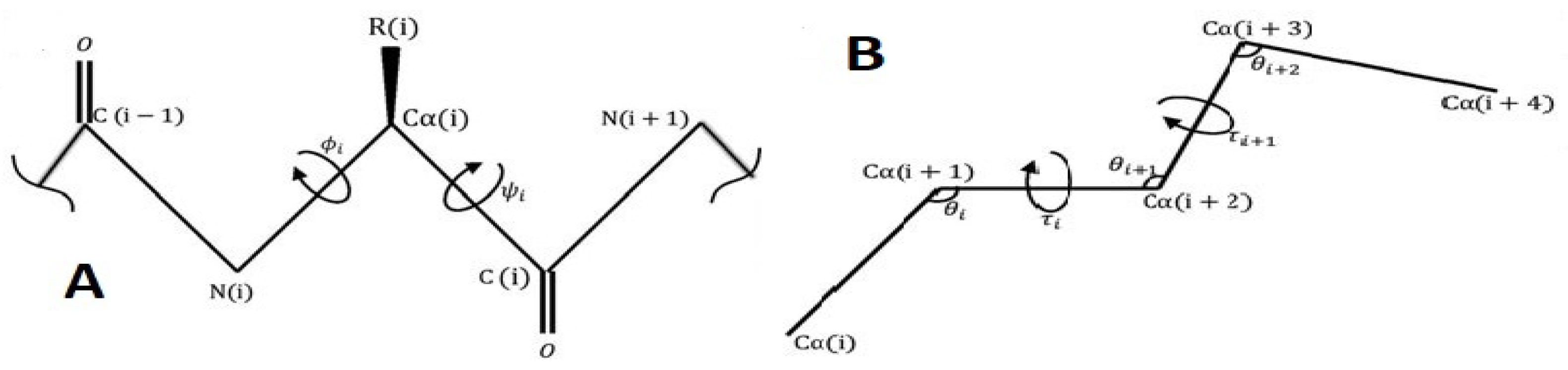
The 3D coordinates of proteins, as provided by electron microscopy, NMR, or X-ray crystallography, directly reveal the conformation of the backbone atoms, with knowledge of standard chemical bond angles and lengths incorporated during the refinement process. Generally, the backbone conformation is analysed using the backbone torsion or the dihedral angles, denoted by $\varphi$, $\psi$, and $\omega$, as introduced by Ramachandran [1] (Figure 1A), where $\omega$ is usually close to ${180}^{\circ }$ or occasionally $0^{\circ }$. Alternatively, virtual bond and torsion angles $\theta$ and $\tau$ may be used to describe a protein backbone representation based on only $C_{\alpha }$ positions (Figure 1B).

Figure 1. Two representations of protein backbone structures based on torsion or pseudo-torsion angles.

A major challenge in molecular biology and computational biochemistry involves predicting protein 3D structure. The encoding gene provides the primary structure of a protein, and the secondary structure may be predicted computationally with high reliability using artificial neural networks [2], based on the propensity of amino acids to form different secondary structures.

However, predicting the 3D structure of a protein, especially if it is larger than 100 amino acids or if a homologue with a known structure and significant sequence identity is not available, remains challenging. This challenge is addressed by de novo structure prediction, which requires parametrized physical force fields. The probability of observing a particular conformation $\mathit{x}$ of the molecule, $p\left(\mathit{x}\right|\beta )$ is considered and expressed as the Boltzmann distribution:

$$p\left(\mathit{x}\right|\beta )=\frac{exp\left(\beta U\right(\mathit{x}\left)\right)}{Z_{\beta }},$$

where $Z_{\beta }$ is the normalization constant, $U\left(\mathit{x}\right)$ is the potential energy of the molecule, $\beta ={\left(k_{b}T\right)}^{-1}$ is the thermodynamic beta, $k_b$ is the Boltzmann constant, and constant T is the temperature. The 3D structure of a molecule can be derived from $p\left(\mathit{x}\right|\beta )$ by determining the mode of the distribution. Molecular dynamics (MD) is a simulation-based method used to probe for the mode of distribution. However, many millions to trillions of steps are required to simulate a single folding event. By contrast with MD, Monte Carlo (MC)-based methods are more time-efficient. In the Markov Chain Monte Carlo (MCMC) method, a Markov chain is constructed using the Metropolis–Hastings (MH) algorithm ([3,4]), with $p\left(\mathbf{x}\right|\beta )$ as the stationary distribution. A symmetric proposal distribution is utilized in the MH algorithm.

Choosing a good proposal distribution is one of the challenges in MCMC-based simulation. Gaussian perturbations are the most straightforward proposal distributions that can be used [5]. The results are more accurate when the proposal distribution is closer to the stationary distribution; therefore, protein structural information is incorporated into most proposal distributions. Using the information on angles and bond lengths observed in real proteins is a simple way to define a suitable proposal distribution. Fragment libraries for backbone angles and rotamer libraries for side-chain angles can be selected as default choices for proposal distributions [6,7,8].

Various tractable statistical distributions for modelling protein dihedral angles are briefly reviewed. These models can be used as proposal distributions for MCMC protein sampling. They can also be utilized as a prior for determining a protein structure from data. However, these models do not generate folded proteins because they work under some simplifying assumptions, both in terms of their functional form and dependency structure (see [9]). The ultimate goal of our contribution is to propose more flexible models for the proposal distribution.

1.1. Brief Overview

An overview of the models available for toroidal data that forms the departure point for the investigation in this paper follows (see [10]).

The first probability distribution on the torus was proposed by Mardia in [11]. It is the bivariate von Mises distribution:

$$\begin{array}{ccc}\hfill f({\theta }_1,{\theta }_2)& =& Cexp({\kappa }_{1}cos({\theta }_1-{\iota }_1)+{\kappa }_{2}cos({\theta }_2-{\iota }_2)\hfill \\ & +& \left(cos({\theta }_1-{\iota }_1),sin({\theta }_1-{\iota }_1)\right)A{\left(cos({\theta }_2-{\iota }_2),sin({\theta }_2-{\iota }_2)\right)}^T),\hfill \end{array}$$

where C is the normalizing constant, ${\iota }_1,{\iota }_2\in [-\pi ,\pi )$ are location parameters, ${\kappa }_1,{\kappa }_2\ge 0$ are concentration parameters, and matrix $A_{2\times 2}$ is the circular–circular dependence parameter. To move beyond the complexity created by the large number of parameters in this founding distribution, a few special cases in the literature have been considered. Rivest in [12] introduced the subclass:

$$\begin{array}{ccc}\hfill f({\theta }_1,{\theta }_2)& \propto & exp({\kappa }_{1}cos({\theta }_1-{\iota }_1)+{\kappa }_{2}cos({\theta }_2-{\iota }_2)+\alpha cos({\theta }_1-{\iota }_1)cos({\theta }_2-{\iota }_2)\hfill \\ \hfill & +& \beta sin({\theta }_1-{\iota }_1)sin({\theta }_2-{\iota }_2)),\hfill \end{array}$$

(1)

where $\alpha ,\beta \in \mathbb{R}$. Singh et al. in [13] proposed the sine model as a special case of (1) with one less parameter, letting $\alpha =0$ and $\beta ={\kappa }_3$:

$$\begin{array}{c}\hfill f({\theta }_1,{\theta }_2)=Cexp({\kappa }_{1}cos({\theta }_1-{\iota }_1)+{\kappa }_{2}cos({\theta }_2-{\iota }_2)+{\kappa }_{3}sin({\theta }_1-{\iota }_1)sin({\theta }_2-{\iota }_2)),\end{array}$$

(2)

where

$$C^{-1}=4{\pi }^2\sum _{i=0}^{\infty }\left(\genfrac{}{}{0pt}{}{2i}{i}\right){\left(\frac{{\kappa }_3^2}{4{\kappa }_1{\kappa }_2}\right)}^i{I}_i\left({\kappa }_1\right)I_i\left({\kappa }_2\right),$$

(3)

where $I_{\alpha }\left(z\right)$ is the modified Bessel function of the first kind of order $\alpha$. Another submodel of (1), the cosine model, was introduced by Mardia et al. in [14] by setting $\alpha =\beta =-{\kappa }_3$:

$$\begin{array}{c}\hfill f({\theta }_1,{\theta }_2)=Cexp({\kappa }_{1}cos({\theta }_1-{\iota }_1)+{\kappa }_{2}cos({\theta }_2-{\iota }_2)-{\kappa }_{3}cos({\theta }_1-{\iota }_1-{\theta }_2+{\iota }_2)),\end{array}$$

(4)

where

$$C^{-1}=4{\pi }^2\left\{I_0\left({\kappa }_1\right)I_0\left({\kappa }_2\right)I_0\left({\kappa }_3\right)+2\sum _{i=1}^{\infty }{I}_i\left({\kappa }_1\right)I_i\left({\kappa }_2\right)I_i\left({\kappa }_3\right)\right\}.$$

(5)

It is worth noting that Kent et al. in [15] introduced another version of the cosine model, with a negative interaction given by:

$$\begin{array}{c}\hfill f({\theta }_1,{\theta }_2)=Cexp({\kappa }_{1}cos({\theta }_1-{\iota }_1)+{\kappa }_{2}cos({\theta }_2-{\iota }_2)-{\kappa }_{3}cos({\theta }_1-{\iota }_1+{\theta }_2-{\iota }_2)),\end{array}$$

with the same normalizing constant as for the model with a positive interaction in (4). Kent et al. in [15] also introduced a submodel of (1), which is a hybrid between the sine and cosine models, given by:

$$\begin{array}{cc}\hfill f({\theta }_1,{\theta }_2)& \propto exp\left({\kappa }_{1}cos({\theta }_1-{\iota }_1)+{\kappa }_{2}cos({\theta }_2-{\iota }_2)\right.\hfill \\ \hfill & \left.+\beta \left\{(cosh\lambda -1)cos({\theta }_1-{\iota }_1)cos({\theta }_2-{\iota }_2))+sinh\lambda sin({\theta }_1-{\iota }_1)sin({\theta }_2-{\iota }_2)\right\}\right),\hfill \end{array}$$

(6)

where ${\kappa }_1,{\kappa }_2\ge 0$, $\lambda \in \mathbb{R}$, and for simplicity, $\beta =1$. Mardia and Frellsen in [16] compared the properties of these three submodels in (2), (4), and (6). The multivariate extensions of the sine model can be found in [17]. In another attempt to expand the platform of toroidal distributions, Wehrly and Johnson in [18] used a marginal specification approach to construct bivariate models with more flexible specified circular marginals. Later, Jones et al. in [19] obtained various toroidal models using the general form in [18]. In this way, Fernández-Durán in [20] proposed another general toroidal model by using a copula pdf that García-Portugués imposed periodic restrictions on in [21], and Jones et al. [19] defined it as a circula pdf, arguing that it is characterised by a circular uniform distribution. For more details, see [22].

The main incentive for defining toroidal models in recent years has been the demand from other sciences, especially bioinformatics, to model dihedral angles in order to analyse protein structures ([13,14,23,24]). However, toroidal data can also be observed in other fields, for example, in meteorology (wind directions at two different times of day) and medicine (peak systolic blood pressure during two separate time periods). For the interested reader, some applications of toroidal models can be found in [25,26,27,28,29].

Most of the proposed toroidal models are pointwise symmetric, whereas the data that they model usually represent asymmetric patterns. This inspired Ameijeiras-Alonso and Ley [24] to introduce bivariate sine-skewed distributions ($BSS$):

$$f_{BSS}({\theta }_1,{\theta }_2)=f({\theta }_1-{\mu }_1,{\theta }_2-{\mu }_2)(1+{\lambda }_{1}sin({\theta }_1-{\mu }_1)+{\lambda }_{2}sin({\theta }_2-{\mu }_2)),$$

(7)

where $f(.,.)$ is a toroidal density symmetric (pointwise) about $-\pi \le {\mu }_1,{\mu }_2<\pi$, and the skewness parameters $-1⩽{\lambda }_i⩽1$, $i=1,2,$ satisfy $|{\lambda }_1|+|{\lambda }_2|⩽1$.

In this paper, Möbius transformation will form the foundation for the construction of competitive models. A map $T:\mathbb{C}\to \mathbb{C}$ is a Möbius transformation if it has the following form:

$$T\left(z\right)=\frac{az+b}{cz+d},$$

where $\mathbb{C}$ is the set of complex numbers, $a,b,c,d\in \mathbb{C}$ are complex numbers, and $ad-bc\ne 0$. Let $S\subset \mathbb{C}$ be a unit circle, then Möbius transformation maps a point on the unit circle $\theta$ onto another $\tilde{\theta }$. Jones in [30] subsequently applied the Möbius transformation to introduce a new family of distributions on the disc. Kato and Jones in [31] used the Möbius transformation to introduce a new distribution on the circle by transforming the von Mises distribution. Wang and Shimizu in [32] applied the Möbius transformation to cardioid random variables. Kato and Pewsey in [33] employed this transformation to define the unimodal bivariate wrapped Cauchy distribution by transforming the bivariate circular distribution in [34]:

$$\begin{array}{cc}\hfill f({\theta }_1,{\theta }_2)& =c\left(c_0-c_{1}cos({\theta }_1-{\mu }_1)-c_{2}cos({\theta }_2-{\mu }_2)-c_{3}cos({\theta }_1-{\mu }_1)cos({\theta }_2-{\mu }_2)\right.\hfill \\ \hfill & {\left.-c_{4}sin({\theta }_1-{\mu }_1)sin({\theta }_2-{\mu }_2)\right)}^{-1},\hfill \end{array}$$

(8)

where $c=(1-{\rho }^2)(1-r_1^2)(1-r_2^2)/4{\pi }^2$, $c_0=(1+{\rho }^2)(1+r_1^2)(1+r_2^2)-8\left|\rho \right|r_1{r}_2$, $c_1=2(1+{\rho }^2)r_1(1+r_2^2)-4\left|\rho \right|(1+r_1^2)r_2$, $c_2=2(1+{\rho }^2)r_2(1+r_2^2)-4\left|\rho \right|(1+r_2^2)r_1$, $c_3=-4(1+{\rho }^2)r_1{r}_2+2\left|\rho \right|(1+r_1^2)(1+r_2^2)$, $c_4=2\rho (1-r_1^2)(1-r_2^2)$, ${\mu }_1,{\mu }_2\in [-\pi ,\pi )$, $r_1,r_2\in [0,1)$, and $-1<\rho <1$. Kato and McCullagh in [35] introduced the Cauchy distribution on the sphere by using a Möbius transformation.

1.2. Our Contribution

In this paper, two new distributions are introduced on the torus by applying a restricted version of the Möbius transformation developed by Kato and Pewsey in [33], namely the circular Möbius transformation that transforms $\theta$ into $\tilde{\theta }$ through the following mapping:

$$\theta =\mho (\tilde{\theta },\mu ,\nu ,r)=\mu +\nu +2arctan\left\{\frac{1-r}{1+r}tan\left(\frac{\tilde{\theta }-\nu }{2}\right)\right\},$$

(9)

where $-\pi \le \mu$, $\nu \le \pi$, $r\in [0,1)$, and $\mu$ is the rotation parameter. When $\mu =0$, $\nu$ and r attract the point $\theta$ towards $\nu$. By increasing r, the concentration of the points around $\nu$ increases. If $r=0$, the transformation is identity mapping, and when $r\to 1$, $\mho (\tilde{\theta },\mu ,\nu ,r)$ tends to $\nu$. More details about the circular Möbius transformation can be found in [29,36]. The inverse of (9) can be obtained as follows:

$$\tilde{\theta }=\nu +2arctan\left\{\frac{1+r}{1-r}tan\left(\frac{\theta -\mu -\nu }{2}\right)\right\}.$$

More specifically, our novel contribution includes the following highlights:

• New Möbius transformation-induced toroidal distributions are developed, acting as alternatives for existing models and efficiently outperforming them in the data application in this paper;
• The proposed distributions reflect the protein structure more accurately than the existing models and can serve as proposal distributions for MCMC sampling of proteins since we should incorporate protein structure information into proposal distributions to obtain more accurate results;
• Sine-skewed versions of these proposed models are introduced to meet the increasing demand for the modelling of asymmetric toroidal data;
• The marginals of the new models lead to new multimodal circular distributions.

The remainder of this paper is organised as follows. Section 2 introduces two new distributions emanating from the sine and cosine models in (2) and (4), respectively. Section 3 introduces the sine-skewed versions of the newly proposed transformed sine and cosine models. Section 4 outlines the maximum likelihood method for obtaining the parameter estimates for the proposed models. Three real datasets, including information on angles in protein structures, are analysed in Section 5 to determine the performance of the proposed models relative to known competitors, and demonstrate their well-deserved designation as possible models for toroidal data. In Section 6, a simulation study is conducted for two reasons: (1) to explore the best method of generating samples from the newly transformed sine and cosine models, and (2) to evaluate the numerical method, followed by the acquisition of the maximum likelihood estimates (MLEs) of the parameters.

2. Two New Models on the Torus

This section highlights two new flexible models for toroidal data, obtained by transforming the sine and cosine models in (2) and (4) via a Möbius transformation.

2.1. Transformed Cosine Model

Let $({\tilde{\mathsf{\Theta }}}_1,{\tilde{\mathsf{\Theta }}}_2)$ have pdf (4) with ${\iota }_1={\iota }_2=0$. Suppose that

$$({\mathsf{\Theta }}_1,{\mathsf{\Theta }}_2)=\left(\mho ({\tilde{\mathsf{\Theta }}}_1,{\mu }_1,{\nu }_1,r_1),\mho ({\tilde{\mathsf{\Theta }}}_2,{\mu }_2,{\nu }_2,r_2)\right),$$

where $\mho (.)$ is defined in (9), ${\mu }_1,{\mu }_2,{\nu }_1,{\nu }_2\in (-\pi ,\pi ]$, $r_1,r_2\in [0,1)$ and without loss of generality ${\nu }_1={\nu }_2=0$. Then, $({\mathsf{\Theta }}_1,{\mathsf{\Theta }}_2)$ has a pdf of

$$\begin{array}{cc}\hfill & f({\theta }_1,{\theta }_2)=\frac{C(1-r_1^2)(1-r_2^2)}{(1+r_1^2-2r_{1}cos({\theta }_1-{\mu }_1))(1+r_2^2-2r_{2}cos({\theta }_2-{\mu }_2))}\hfill \\ \hfill & \times exp\left\{\frac{1}{(1+r_1^2-2r_{1}cos({\theta }_1-{\mu }_1))(1+r_2^2-2r_{2}cos({\theta }_2-{\mu }_2))}\left(C_0+C_{1}cos({\theta }_1-{\mu }_1)\right.\right.\hfill \\ \hfill & \left.\left.+C_{2}cos({\theta }_2-{\mu }_2)+C_{3}cos({\theta }_1-{\mu }_1)cos({\theta }_2-{\mu }_2)+C_{4}sin({\theta }_1-{\mu }_1)sin({\theta }_2-{\mu }_2)\right)\right\},\hfill \end{array}$$

(10)

where ${\kappa }_1,{\kappa }_2\ge 0$, ${\kappa }_3\in \mathbb{R}$, C is defined in (5), and

$$\begin{array}{cc}\hfill C_0& =-2{\kappa }_1{r}_1(1+r_2^2)-2{\kappa }_2{r}_2(1+r_1^2)-4{\kappa }_3{r}_1{r}_2,\hfill \\ \hfill C_1& ={\kappa }_1(1+r_1^2)(1+r_2^2)+2{\kappa }_3{r}_2(1+r_1^2)+4{\kappa }_2{r}_1{r}_2,\hfill \\ \hfill C_2& ={\kappa }_2(1+r_1^2)(1+r_2^2)+2{\kappa }_3{r}_1(1+r_2^2)+4{\kappa }_1{r}_1{r}_2,\hfill \\ \hfill C_3& =-2{\kappa }_1{r}_2(1+r_1^2)-2{\kappa }_2{r}_1(1+r_2^2)-{\kappa }_3(1+r_1^2)(1+r_2^2),\hfill \\ \hfill C_4& =-{\kappa }_3(1-r_1^2)(1-r_2^2),\hfill \end{array}$$

(11)

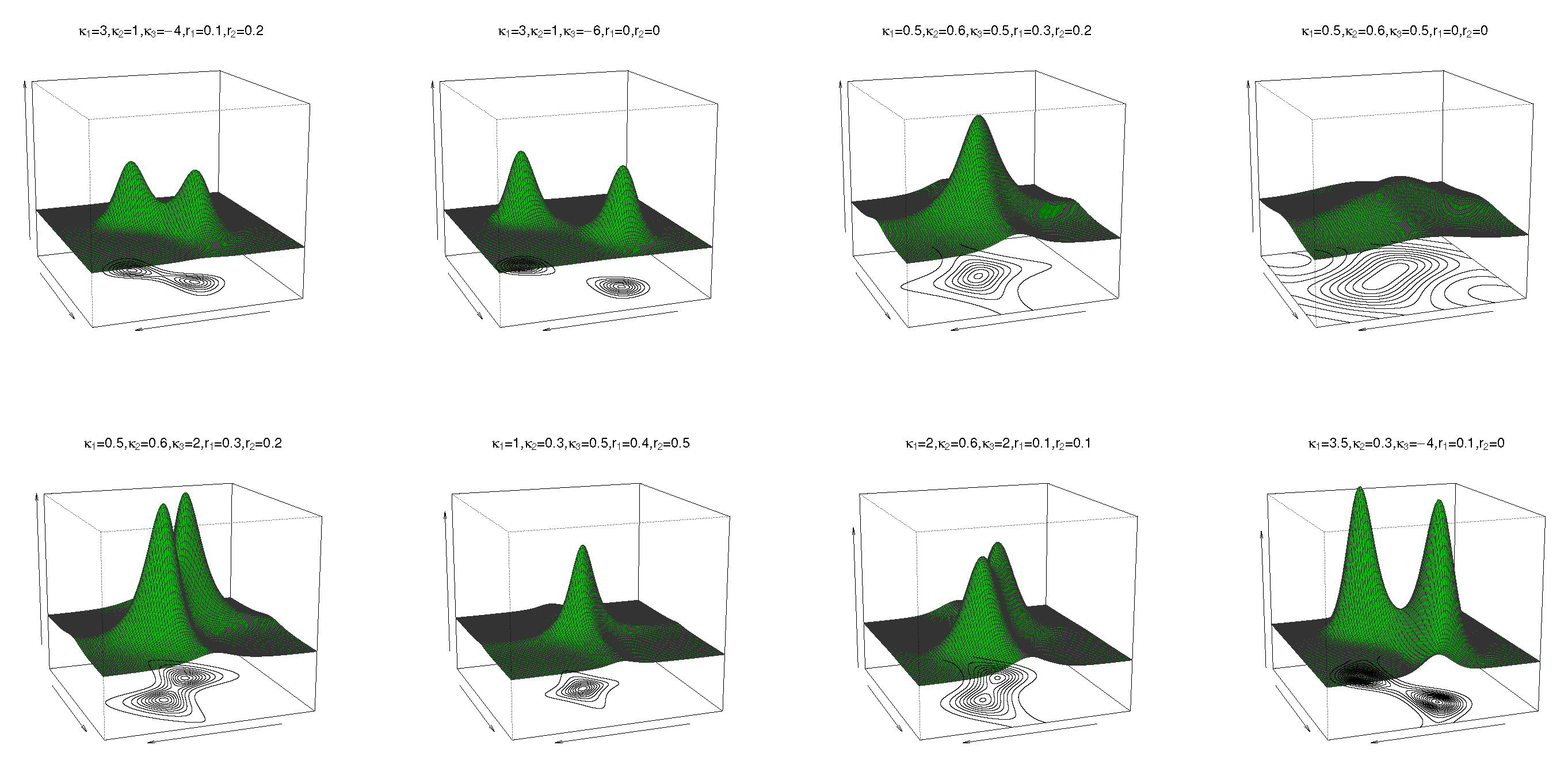
where ${\mu }_1,{\mu }_2\in [-\pi ,\pi )$ are location parameters, ${\kappa }_1,{\kappa }_2\ge 0$ are concentration parameters, ${\kappa }_3$ is the circular–circular dependence parameter, and $r_1$ and $r_2$ regulate the concentrations of the marginal distributions. In (10), when $r_1=r_2=0$, the cosine model (4) is obtained. If ${\kappa }_1,{\kappa }_2,{\kappa }_3=0$ yields the bivariate wrapped Cauchy distribution, then ${\theta }_1\perp {\theta }_2$ follows. The pdf and contour plots of (10) are shown in Figure 2 for ${\mu }_1={\mu }_2=0$ and different values of ${\kappa }_1,{\kappa }_2,{\kappa }_3,r_1$ and $r_2$, and reveal unimodal and bimodal behaviour.

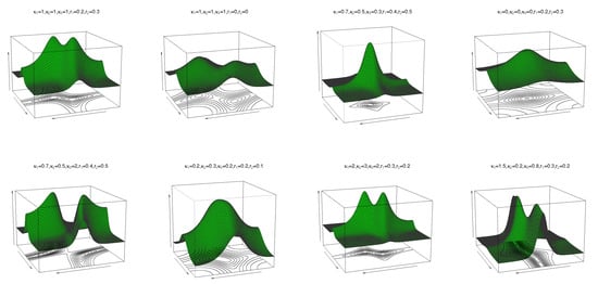
Figure 2. Pdf and contour plots of the transformed cosine model (10) for ${\mu }_1={\mu }_2=0$ and different values of ${\kappa }_1,{\kappa }_2,{\kappa }_3,r_1$, and $r_2$.

Proposition 1.

Assuming the transformed cosine model (10), when $r_1,r_2\to 0$, then $({\mathsf{\Theta }}_1,{\mathsf{\Theta }}_2)$ has approximately a bivariate normal distribution if and only if ${\kappa }_3\le \frac{{\kappa }_1{\kappa }_2}{{\kappa }_1+{\kappa }_2}$.

Proof. 

See Appendix A. □

In the following, the marginal pdf and conditional pdf of the transformed cosine model (10) and their properties are discussed. The marginal pdf of ${\theta }_1$ for the transformed cosine model in (10) is as follows:

$$\begin{array}{c}\hfill f_{{\mathsf{\Theta }}_1}\left({\theta }_1\right)=\frac{2\pi C(1-r_1^2)}{1+r_1^2-2r_{1}cos({\theta }_1-{\mu }_1)}{I}_0\left(h\left({\theta }_1\right)\right)exp\left\{\frac{{\kappa }_1(1+r_1^2)cos({\theta }_1-{\mu }_1)-2{\kappa }_1{r}_1}{1+r_1^2-2r_{1}cos({\theta }_1-{\mu }_1)}\right\},\end{array}$$

(12)

where

$$h\left({\theta }_1\right)={\left\{{\kappa }_2^2+{\kappa }_3^2-\frac{2{\kappa }_2{\kappa }_3\left((1+r_1^2)cos({\theta }_1-{\mu }_1)-2r_1\right)}{1+r_1^2-2r_{1}cos({\theta }_1-{\mu }_1)}\right\}}^{1/2},$$

(13)

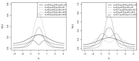
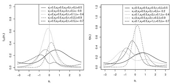
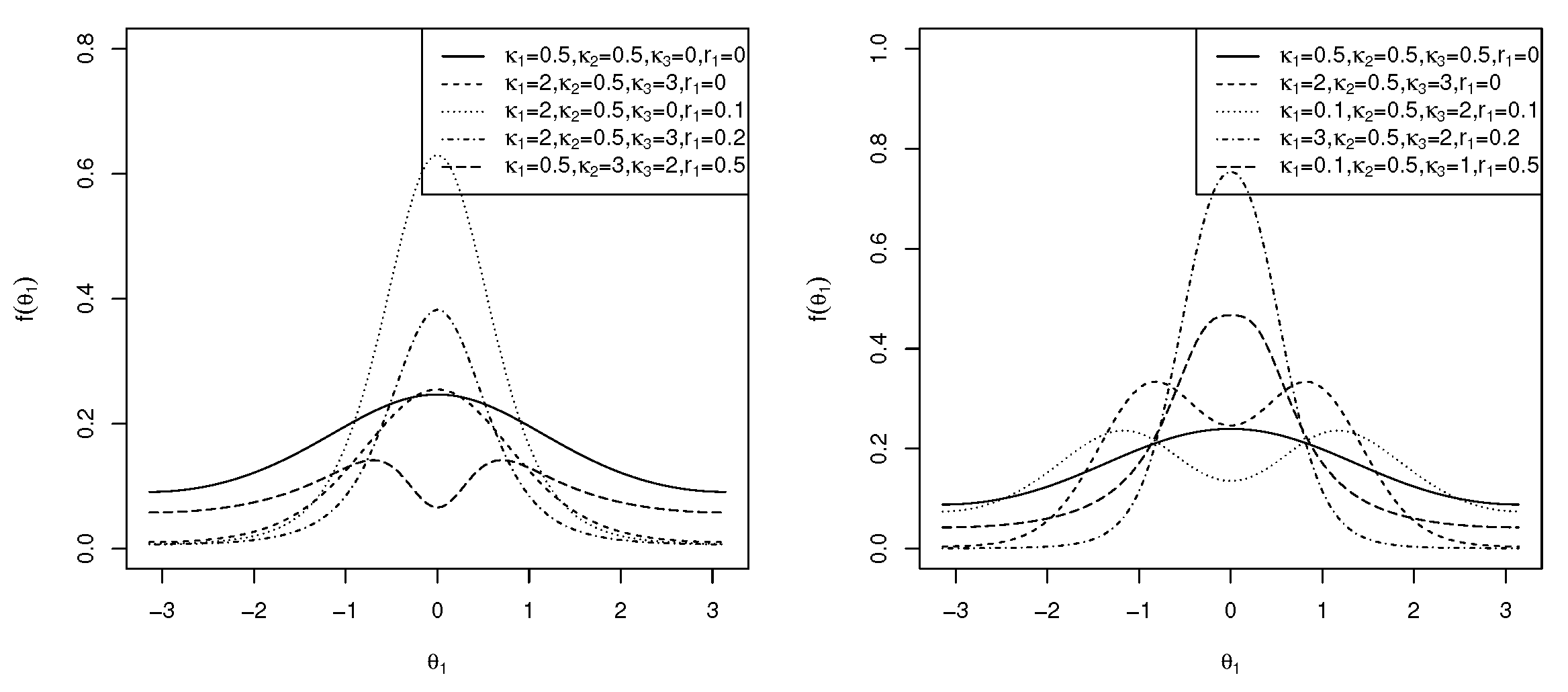
and C is as defined in (5). The marginal pdf of ${\mathsf{\Theta }}_1$ in (12) is symmetric to ${\mu }_1$, small values of ${\kappa }_3$ approximate the transformed von Mises distribution [31], and $r_1=0$, which simplifies to the marginal pdf of the cosine model [14]. It is clear that for $r_1=0$ and small values of ${\kappa }_3$, the von Mises distribution is approximated. If ${\kappa }_1={\kappa }_2={\kappa }_3=0$ in (12), then the Möbius-transformed uniform distribution is obtained. For ${\kappa }_1={\kappa }_2={\kappa }_3=r_1=0$, the distribution is uniform. When ${\kappa }_1={\kappa }_2=0$ in (12), the distribution is the transformed von Mises distribution [31], and when ${\kappa }_1={\kappa }_2=r_1=0$, the von Mises distribution is obtained. The plots of this generalized marginal pdf of ${\mathsf{\Theta }}_1$ are shown in Figure 3 (left) for ${\mu }_1=0$ and different values of ${\kappa }_1,{\kappa }_2,{\kappa }_3$ and $r_1$, reflecting unimodal and bimodal graphs. In the following theorem, the modality of the marginal density function ${\mathsf{\Theta }}_1$ is addressed.

Figure 3. Plots of the marginal pdf of ${\mathsf{\Theta }}_1$ in (12) (left) and in (18) (right) for ${\mu }_1=0$ and different parameter values.

Corollary 1.

The marginal distribution of ${\mathsf{\Theta }}_1$ in (12) is symmetric around ${\theta }_1={\mu }_1$ and unimodal (with mode at ${\mu }_1$) if and only if $\frac{A(\mid {\kappa }_2-{\kappa }_3\mid )}{\mid {\kappa }_2-{\kappa }_3\mid }\le \left(\frac{2r_1{(1-r_1)}^2}{{(1-r_1^2)}^2}+{\kappa }_1\right)/{\kappa }_2{\kappa }_3$, where $A\left(\kappa \right)=I_1\left(\kappa \right)/I_0\left(\kappa \right)$. Moreover, the marginal distribution of ${\mathsf{\Theta }}_1$ in (12) is bimodal (with the modes at ${\mu }_1-{\theta }_1^{*}$ and ${\mu }_1+{\theta }_1^{*}$) if and only if $\frac{A(\mid {\kappa }_2-{\kappa }_3\mid )}{\mid {\kappa }_2-{\kappa }_3\mid }>\left(\frac{2r_1{(1-r_1)}^2}{{(1-r_1^2)}^2}+{\kappa }_1\right)/{\kappa }_2{\kappa }_3$, and ${\theta }_1^{*}$ is the root of ${\kappa }_2{\kappa }_3{(1-r_1^2)}^{2}A\left(h\left({\theta }_1^{*}\right)\right)/$$h\left({\theta }_1^{*}\right)-2r_1(1+r_1^2-2r_{1}cos({\theta }_1^{*}-{\mu }_1))-{\kappa }_1{(1-r_1^2)}^2=0$, where $h\left(\theta \right)$ is as defined in (13).

Proof. 

See Appendix A. □

The conditional pdf $f({\theta }_2\mid {\mathsf{\Theta }}_1={\theta }_1)$ results in the transformed von Mises distribution [31] given by the following:

$$\begin{array}{cc}\hfill & f({\theta }_2\mid {\mathsf{\Theta }}_1={\theta }_1)=\frac{1-r_2^2}{2\pi I_0\left(h\left({\theta }_1\right)\right)}\frac{1}{1+r_2^2-2r_{2}cos({\theta }_2-{\mu }_2)}\hfill \\ \hfill & \times exp\left\{\frac{h\left({\theta }_1\right)cos\tau ((1+r_2^2)cos({\theta }_2-{\mu }_2)-2r_2)+h\left({\theta }_1\right)sin\tau (1-r_2^2)sin({\theta }_2-{\mu }_2)}{1+r_2^2-2r_{2}cos({\theta }_2-{\mu }_2)}\right\},\hfill \end{array}$$

(14)

where $h\left({\theta }_1\right)$ is as defined in (13), and

$$tan\tau =\frac{-{\kappa }_3(1-r_1^2)sin({\theta }_1-{\mu }_1)}{{\kappa }_2(1+r_1^2-2r_{1}cos({\theta }_1-{\mu }_1))-{\kappa }_3((1+r_1^2)cos({\theta }_1-{\mu }_1)-2r_1)}$$

(15)

Note that for $r_1=r_2=0$, (14) simplifies to the von Mises distribution with the parameters $\tau$ and $h\left({\theta }_1\right)$ in (13).

2.2. Transformed Sine Model

Let $({\tilde{\mathsf{\Theta }}}_1,{\tilde{\mathsf{\Theta }}}_2)$ have a bivariate pdf (2), with ${\iota }_1={\iota }_2=0$. Suppose that

$$({\mathsf{\Theta }}_1,{\mathsf{\Theta }}_2)=\left(\mho ({\tilde{\mathsf{\Theta }}}_1,{\mu }_1,{\nu }_1,r_1),\mho ({\tilde{\mathsf{\Theta }}}_2,{\mu }_2,{\nu }_2,r_2)\right),$$

where $\mho (.)$ is as defined in (9), ${\mu }_1,{\mu }_2,{\nu }_1,{\nu }_2\in (-\pi ,\pi ]$, $r_1,r_2\in [0,1)$, and without loss of generality ${\nu }_1={\nu }_2=0$. Then, $({\mathsf{\Theta }}_1,{\mathsf{\Theta }}_2)$ has a pdf as follows:

$$\begin{array}{cc}\hfill & f({\theta }_1,{\theta }_2)=\frac{C(1-r_1^2)(1-r_2^2)}{(1+r_1^2-2r_{1}cos({\theta }_1-{\mu }_1))(1+r_2^2-2r_{2}cos({\theta }_2-{\mu }_2))}\hfill \\ \hfill & \times exp\left\{\frac{1}{(1+r_1^2-2r_{1}cos({\theta }_1-{\mu }_1))(1+r_2^2-2r_{2}cos({\theta }_2-{\mu }_2))}\left(C_0+C_{1}cos({\theta }_1-{\mu }_1)\right.\right.\hfill \\ \hfill & \left.\left.+C_{2}cos({\theta }_2-{\mu }_2)+C_{3}cos({\theta }_1-{\mu }_1)cos({\theta }_2-{\mu }_2)+C_{4}sin({\theta }_1-{\mu }_1)sin({\theta }_2-{\mu }_2)\right)\right\},\hfill \end{array}$$

(16)

where ${\kappa }_1,{\kappa }_2\ge 0$, ${\kappa }_3\in \mathbb{R}$, C is as defined in (3), and

$$\begin{array}{cc}\hfill C_0& =-2{\kappa }_1{r}_1(1+r_2^2)-2{\kappa }_2{r}_2(1+r_1^2),\hfill \\ \hfill C_1& ={\kappa }_1(1+r_1^2)(1+r_2^2)+4{\kappa }_2{r}_1{r}_2,\hfill \\ \hfill C_2& ={\kappa }_2(1+r_1^2)(1+r_2^2)+4{\kappa }_1{r}_1{r}_2,\hfill \\ \hfill C_3& =-2{\kappa }_1{r}_2(1+r_1^2)-2{\kappa }_2{r}_1(1+r_2^2),\hfill \\ \hfill C_4& ={\kappa }_3(1-r_1^2)(1-r_2^2),\hfill \end{array}$$

(17)

where ${\mu }_1,{\mu }_2\in [-\pi ,\pi )$ are location parameters, ${\kappa }_1,{\kappa }_2\ge 0$ are concentration parameters, ${\kappa }_3$ is the circular–circular dependence parameter, and $r_1$ and $r_2$ regulate the concentrations of the marginal distributions. If $r_1=r_2=0$ in (16), then the sine model in (2) follows. The pdf and contour plots of (16) are shown in Figure 4 for ${\mu }_1={\mu }_2=0$ and for different values of ${\kappa }_1,{\kappa }_2,{\kappa }_3,r_1$ and $r_2$. As can be seen, this transformed sine pdf (16) can have both unimodal and bimodal forms.

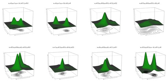
Figure 4. Pdf and contour plots of the transformed sine model (16) for ${\mu }_1={\mu }_2=0$ and different values of ${\kappa }_1,{\kappa }_2,{\kappa }_3,r_1$, and $r_2$.

Proposition 2.

Assuming the transformed sine model in (16), when $r_1,r_2\to 0$, then $({\mathsf{\Theta }}_1,{\mathsf{\Theta }}_2)$ has an approximately bivariate normal distribution if and only if ${\kappa }_3^2<{\kappa }_1{\kappa }_2$.

Proof. 

Similarly, Theorem 1 is proved using the results in [13]. □

In this case, the marginal pdf of ${\mathsf{\Theta }}_1$ for the transformed sine model in (16) is as follows:

$$\begin{array}{c}\hfill f_{{\mathsf{\Theta }}_1}\left({\theta }_1\right)=\frac{2\pi C(1-r_1^2)}{1+r_1^2-2r_{1}cos({\theta }_1-{\mu }_1)}{I}_0\left(h\left({\theta }_1\right)\right)exp\left\{\frac{{\kappa }_1(1+r_1^2)cos({\theta }_1-{\mu }_1)-2{\kappa }_1{r}_1}{1+r_1^2-2r_{1}cos({\theta }_1-{\mu }_1)}\right\},\end{array}$$

(18)

where

$$h\left({\theta }_1\right)={\left\{{\kappa }_2^2+{\left(\frac{{\kappa }_3(1-r_1^2)}{1+r_1^2-2r_{1}cos({\theta }_1-{\mu }_1)}\right)}^2{sin}^2({\theta }_1-{\mu }_1)\right\}}^{1/2},$$

(19)

and C, as shown in (3). The marginal pdf of ${\mathsf{\Theta }}_1$ is symmetric around ${\mu }_1$. If ${\kappa }_3=0$, the distribution is the transformed von Mises distribution [31]. If $r_1=0$ in (18), the marginal distribution of the sine model [13] is obtained. The plots of the marginal pdf of ${\mathsf{\Theta }}_1$ in (18) are shown in Figure 3 (right) for ${\mu }_1=0$ and different values of ${\kappa }_1,{\kappa }_2,{\kappa }_3$, and $r_1$. As can be seen, the distribution can be both unimodal and bimodal. In the following theorem, the modality of the marginal pdf of ${\mathsf{\Theta }}_1$ in (18) is explored.

Corollary 2.

The marginal distribution of ${\mathsf{\Theta }}_1$ in (18) is symmetric around ${\theta }_1={\mu }_1$ and unimodal (with mode at ${\mu }_1$) if and only if $\frac{A\left({\kappa }_2\right)}{{\kappa }_2}\le \left(\frac{2r_1{(1-r_1)}^2}{{(1-r_1^2)}^2}+{\kappa }_1\right)/{\kappa }_3^2$, where $A\left(\kappa \right)=I_1\left(\kappa \right)/I_0\left(\kappa \right)$. Moreover, the marginal distribution of ${\mathsf{\Theta }}_1$ in (18) is bimodal (with the modes at ${\mu }_1-{\theta }_1^{*}$ and ${\mu }_1+{\theta }_1^{*}$) if and only if $\frac{A\left({\kappa }_2\right)}{{\kappa }_2}>\left(\frac{2r_1{(1-r_1)}^2}{{(1-r_1^2)}^2}+{\kappa }_1\right)/{\kappa }_3^2$, and ${\theta }_1^{*}$ is the root of ${\kappa }_3^2{(1-r_1^2)}^{2}cos{\theta }_1^{*}A\left(h\left({\theta }_1^{*}\right)\right)/h\left({\theta }_1^{*}\right)-2r_1(1+r_1^2-2r_{1}cos({\theta }_1^{*}-{\mu }_1))-{\kappa }_1{(1-r_1^2)}^2=0$, where $h\left(\theta \right)$ is as defined in (19).

Proof. 

See Appendix A. □

The conditional pdf $f({\theta }_2\mid {\mathsf{\Theta }}_1={\theta }_1)$ is given by:

$$\begin{array}{cc}\hfill & f({\theta }_2\mid {\mathsf{\Theta }}_1={\theta }_1)=\frac{1-r_2^2}{2\pi I_0\left(h\left({\theta }_1\right)\right)}\frac{1}{1+r_2^2-2r_{2}cos({\theta }_2-{\mu }_2)}\hfill \\ \hfill & \times exp\left\{\frac{h\left({\theta }_1\right)cos\tau ((1+r_2^2)cos({\theta }_2-{\mu }_2)-2r_2)+h\left({\theta }_1\right)sin\tau (1-r_2^2)sin({\theta }_2-{\mu }_2)}{1+r_2^2-2r_{2}cos({\theta }_2-{\mu }_2)}\right\},\hfill \end{array}$$

(20)

where $h\left({\theta }_1\right)$ is as defined in (19), and

$$tan\tau =\frac{{\kappa }_3}{{\kappa }_2}\frac{(1-r_1^2)sin({\theta }_1-{\mu }_1)}{1+r_1^2-2r_{1}cos({\theta }_1-{\mu }_1)}$$

(21)

Interestingly, the conditional distribution is the transformed von Mises distribution [31]. When $r_1=r_2=0$ in (20), the von Mises distribution with parameters $\tau$ and $h\left({\theta }_1\right)$ is obtained.

3. Sine-Skewed Transformed Sine and Cosine Distributions

In practice, it is possible to have skewed toroidal datasets, despite the well-known toroidal distributions being pointwise symmetric. Therefore, it would be interesting to extend this methodology to the recent model of Ameijeiras-Alonso and Ley in [24]. In this section, the skewed versions of the proposed transformed sine and cosine models in (16) and (10) are introduced. In addition, Abe and Pewsey’s skew model in [37] is applied to extend models on the circle manifold using marginal density functions.

By substituting (10) in (7), the sine-skewed transformed cosine ($BSSTC$) distribution can be defined as follows:

$$\begin{array}{cc}\hfill & f_{BSSTC}({\theta }_1,{\theta }_2)=\frac{C(1-r_1^2)(1-r_2^2)}{(1+r_1^2-2r_{1}cos({\theta }_1-{\mu }_1))(1+r_2^2-2r_{2}cos({\theta }_2-{\mu }_2))}\hfill \\ \hfill & \times exp\left\{\frac{1}{(1+r_1^2-2r_{1}cos({\theta }_1-{\mu }_1))(1+r_2^2-2r_{2}cos({\theta }_2-{\mu }_2))}\left(C_0+C_{1}cos({\theta }_1-{\mu }_1)\right.\right.\hfill \\ \hfill & \left.\left.+C_{2}cos({\theta }_2-{\mu }_2)+C_{3}cos({\theta }_1-{\mu }_1)cos({\theta }_2-{\mu }_2)+C_{4}sin({\theta }_1-{\mu }_1)sin({\theta }_2-{\mu }_2)\right)\right\}\hfill \\ \hfill & \times \left(1+{\lambda }_{1}sin({\theta }_1-{\mu }_1)+{\lambda }_{2}sin({\theta }_2-{\mu }_2)\right),\hfill \end{array}$$

(22)

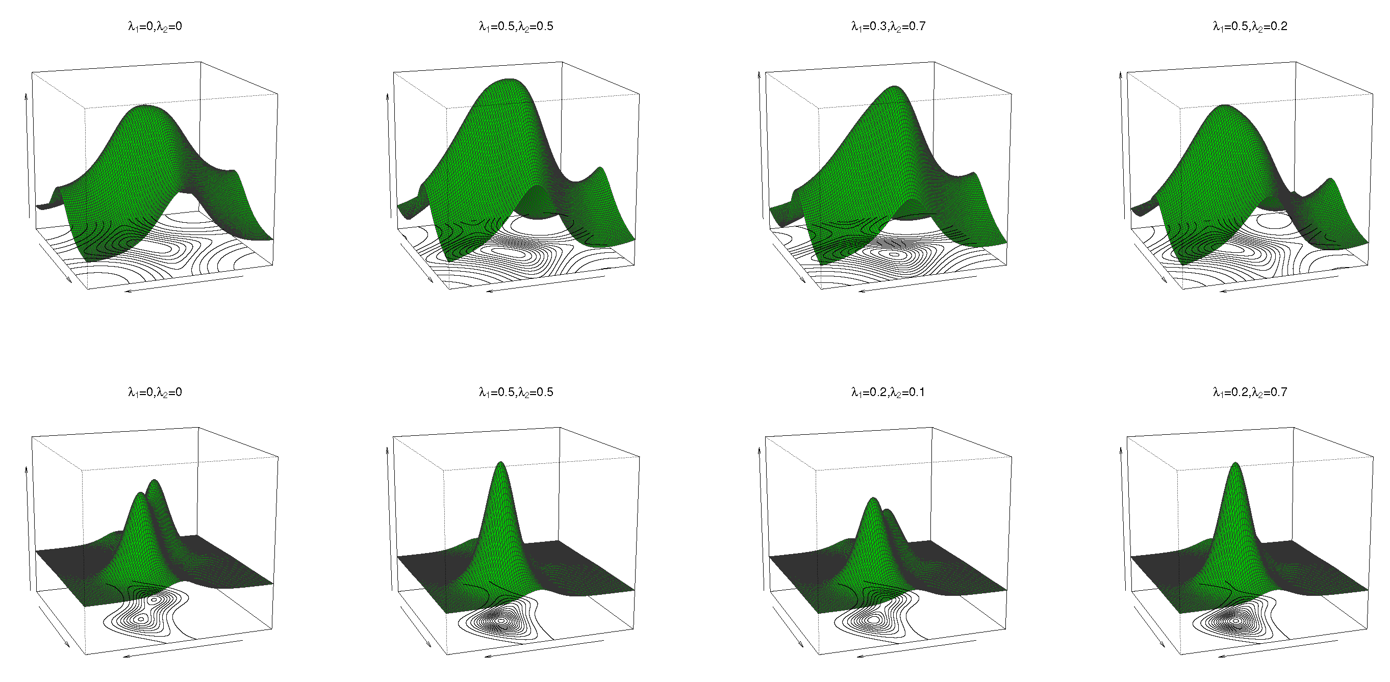
where ${\kappa }_1,{\kappa }_2\ge 0$, ${\kappa }_3\in \mathbb{R}$, C is as defined in (5), and $C_0$–$C_4$ are as defined in (11). The pdf and contour plots of the sine-skewed transformed cosine model for ${\kappa }_1=0.2$, ${\kappa }_2=0.3$, ${\kappa }_3=0.2$, $r_1=0.2$, $r_2=0.1$, ${\mu }_1={\mu }_2=0$, and different values of ${\lambda }_1$ and ${\lambda }_2$ are shown in Figure 5 (top).

Figure 5. Pdf and contour plots of the sine-skewed transformed cosine model in (22) (top) and the sine-skewed transformed sine model in (24) (bottom) for different values of ${\lambda }_1$ and ${\lambda }_2$.

The marginal pdf of ${\theta }_1$ for $BSSTC$ in (22) is as follows:

$$\begin{array}{cc}\hfill & f_{{\mathsf{\Theta }}_1;BSS}\left({\theta }_1\right)=\frac{C(1-r_1^2)}{1+r_1^2-2r_{1}cos({\theta }_1-{\mu }_1)}exp\left\{\frac{{\kappa }_1(1+r_1^2)cos({\theta }_1-{\mu }_1)-2{\kappa }_1{r}_1}{1+r_1^2-2r_{1}cos({\theta }_1-{\mu }_1)}\right\}\hfill \\ \hfill & \times \left\{2\pi I_0\left(h\left({\theta }_1\right)\right)\left(1+{\lambda }_1(1-r_1^2)sin({\theta }_1-{\mu }_1)/\left(1+r_1^2-2r_{1}cos({\theta }_1-{\mu }_1)\right)\right)\right.\hfill \\ \hfill & \left.+{\lambda }_{2}A\left(h\left({\theta }_1\right)\right)cos(\tau +{\mu }_2)\right\}\hfill \end{array}$$

(23)

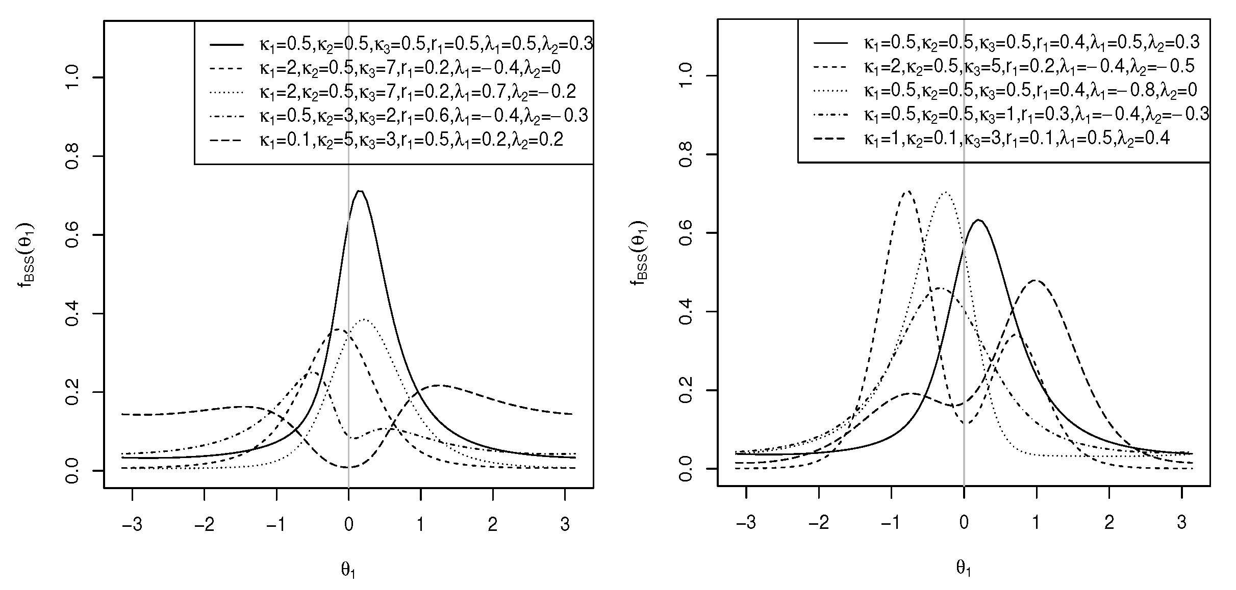
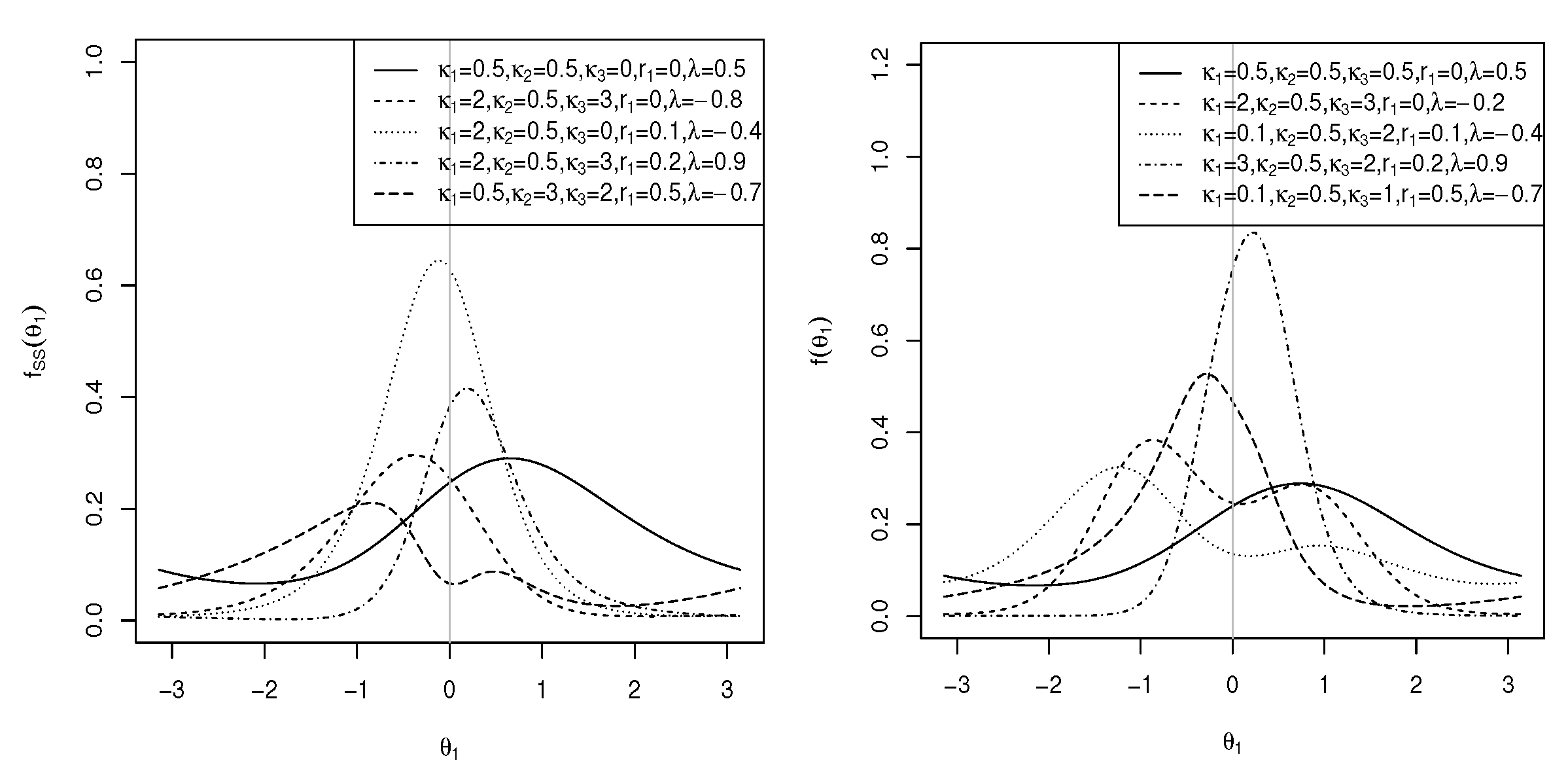
where $h\left({\theta }_1\right)$ and $\tau$ are obtained from (13) and (15), respectively. When ${\lambda }_2=0$, $f_{{\mathsf{\Theta }}_1;BSS}\left({\theta }_1\right)$ is the Möbius-transformed sine-skewed version [37] of the marginal pdf of the cosine model. The plots of the skewed pdf in (23) are shown in Figure 6 (left) for ${\mu }_1={\mu }_2=0$ and different values of ${\kappa }_1,{\kappa }_2,{\kappa }_3,r_1,{\lambda }_1$, and ${\lambda }_2$. As can be observed, the distribution can be both unimodal and bimodal.

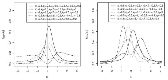
Figure 6. Plots of the marginal pdf of ${\mathsf{\Theta }}_1$ for $BSSTC$ (left) and $BSSTS$ (right) for ${\mu }_1={\mu }_2=0$ and different parameter values.

Similarly, from (16) and (7), the sine-skewed transformed sine ($BSSTS$) distribution can be obtained as follows:

$$\begin{array}{cc}\hfill & f_{BSSTS}({\theta }_1,{\theta }_2)=\frac{C(1-r_1^2)(1-r_2^2)}{(1+r_1^2-2r_{1}cos({\theta }_1-{\mu }_1))(1+r_2^2-2r_{2}cos({\theta }_2-{\mu }_2))}\hfill \\ \hfill & \times exp\left\{\frac{1}{(1+r_1^2-2r_{1}cos({\theta }_1-{\mu }_1))(1+r_2^2-2r_{2}cos({\theta }_2-{\mu }_2))}\left(C_0+C_{1}cos({\theta }_1-{\mu }_1)\right.\right.\hfill \\ \hfill & \left.\left.+C_{2}cos({\theta }_2-{\mu }_2)+C_{3}cos({\theta }_1-{\mu }_1)cos({\theta }_2-{\mu }_2)+C_{4}sin({\theta }_1-{\mu }_1)sin({\theta }_2-{\mu }_2)\right)\right\}\hfill \\ \hfill & \times \left(1+{\lambda }_{1}sin({\theta }_1-{\mu }_1)+{\lambda }_{2}sin({\theta }_2-{\mu }_2)\right),\hfill \end{array}$$

(24)

where ${\kappa }_1,{\kappa }_2\ge 0$, ${\kappa }_3\in \mathbb{R}$, C is as defined in (3), and $C_0$–$C_4$ are defined in (17). The pdf and contour plots of the sine-skewed transformed sine model for ${\kappa }_1=2$, ${\kappa }_2=0.6$, ${\kappa }_3=2$, $r_1=0.1$, $r_2=0.1$, ${\mu }_1={\mu }_2=0$, and different values of ${\lambda }_1$ and ${\lambda }_2$ are shown in Figure 5 (bottom).

The marginal pdf of ${\theta }_1$ for $BSSTS$ is of the same density as in (23), where $h\left({\theta }_1\right)$ and $\tau$ are obtained from (19) and (21). When ${\lambda }_2=0$, $f_{{\theta }_1;BSS}\left({\theta }_1\right)$ is the Möbius-transformed sine-skewed version [37] of the marginal pdf of the sine model. The plots of the skewed pdf in (23) are shown in Figure 6 (right) for ${\mu }_1={\mu }_2=0$ and different values of ${\kappa }_1,{\kappa }_2,{\kappa }_3,r_1,{\lambda }_1$, and ${\lambda }_2$. Figure 6 illustrates that the distribution can have both unimodal and bimodal forms.

To expand the skewed circular models, the following models are introduced based on the k sine-skewed model of [37]. The skewed version of the marginal distribution of ${\mathsf{\Theta }}_1$ in (12) is the following:

$$\begin{array}{cc}\hfill f_{SS}\left({\theta }_1\right)& =\frac{2\pi C(1-r_1^2)}{1+r_1^2-2r_{1}cos({\theta }_1-{\mu }_1)}{I}_0\left(h\left({\theta }_1\right)\right)exp\left\{\frac{{\kappa }_1(1+r_1^2)cos({\theta }_1-{\mu }_1)-2{\kappa }_1{r}_1}{1+r_1^2-2r_{1}cos({\theta }_1-{\mu }_1)}\right\}\hfill \\ \hfill & \times (1+\lambda sin\left(k({\theta }_1-{\mu }_1)\right)),\hfill \end{array}$$

(25)

where C is as defined in (5), $h\left({\theta }_1\right)$ is as defined in (13), and $-1\le \lambda \le 1$. $\lambda >0$ leads to left-skewed distributions, and $\lambda <0$ provides right-skewed distributions. The plots of the skewed pdf in (25) are shown in Figure 7 (left) for $k=1$, ${\mu }_1=0$, and different values of ${\kappa }_1,{\kappa }_2,{\kappa }_3,r_1$, and $\lambda$.

Figure 7. Plots of the sine-skewed versions of marginal pdfs of ${\mathsf{\Theta }}_1$ in (12) (left) and (18) (right) for $k=1$, ${\mu }_1=0$ and different parameter values.

Similarly, the sine-skewed version [37] of the marginal pdf of ${\mathsf{\Theta }}_1$ in (18) is of the same density as in (25), where C is as defined in (3), $h\left({\theta }_1\right)$ is as defined in (19), and $-1\le \lambda \le 1$. The plots of the sine-skewed version of the marginal pdf in (18) are shown in Figure 7 (right) for $k=1$, ${\mu }_1=0$, and different values of ${\kappa }_1,{\kappa }_2,{\kappa }_3,r_1$, and $\lambda$. As can be seen, the distribution is both unimodal and bimodal. Multimodal results for $k>1$.

4. Maximum Likelihood Estimation

In this section, the maximum likelihood method is outlined to obtain the estimates of parameters for both the transformed cosine and sine models. Suppose that $\mathbf{\zeta }={({\mu }_1,{\mu }_2,{\kappa }_1,{\kappa }_2,{\kappa }_3,r_1,r_2)}^T$ are the parameters associated with the transformed cosine model (10). The log-likelihood function of the transformed cosine model is represented as follows:

$$\begin{array}{c}l\left(\mathbf{\zeta }\right)=nlogC+nlog(1-r_1^2)+nlog(1-r_2^2)-{\displaystyle \sum _{i=1}^n}log(1+r_1^2-2r_{1}cos({\theta }_{1i}-{\mu }_1))\hfill \\ -{\displaystyle \sum _{i=1}^n}log(1+r_2^2-2r_{2}cos({\theta }_{2i}-{\mu }_2))+{\displaystyle \sum _{i=1}^n}\frac{1}{(1+r_1^2-2r_{1}cos({\theta }_{1i}-{\mu }_1))(1+r_2^2-2r_{2}cos({\theta }_{2i}-{\mu }_2))}\hfill \\ \times \left(C_0+C_{1}cos({\theta }_{1i}-{\mu }_1)+C_{2}cos({\theta }_{2i}-{\mu }_2)+C_{3}cos({\theta }_{1i}-{\mu }_1)cos({\theta }_{2i}-{\mu }_2)\right.\hfill \\ \left.+C_{4}sin({\theta }_{1i}-{\mu }_1)sin({\theta }_{2i}-{\mu }_2)\right),\hfill \end{array}$$

(26)

where C is as defined in (5), and $C_0$–$C_4$ are as defined in (11). The MLE of the parameters, $\widehat{\mathbf{\zeta }}={({\widehat{\mu }}_1,{\widehat{\mu }}_2,{\widehat{\kappa }}_1,{\widehat{\kappa }}_2,{\widehat{\kappa }}_3,{\widehat{r}}_1,{\widehat{r}}_2)}^T$, can be determined by maximizing (26) with respect to $\mathbf{\zeta }={({\mu }_1,{\mu }_2,{\kappa }_1,{\kappa }_2,{\kappa }_3,r_1,r_2)}^T$.

Supposing that $\mathbf{\zeta }={({\mu }_1,{\mu }_2,{\kappa }_1,{\kappa }_2,{\kappa }_3,r_1,r_2)}^T$ are the parameters associated with the transformed sine model (16), the log-likelihood function of the transformed sine model can be represented as follows:

$$\begin{array}{c}l\left(\mathbf{\zeta }\right)=nlogC+nlog(1-r_1^2)+nlog(1-r_2^2)-{\displaystyle \sum _{i=1}^n}log(1+r_1^2-2r_{1}cos({\theta }_{1i}-{\mu }_1))\hfill \\ -{\displaystyle \sum _{i=1}^n}log(1+r_2^2-2r_{2}cos({\theta }_{2i}-{\mu }_2))+{\displaystyle \sum _{i=1}^n}\frac{1}{(1+r_1^2-2r_{1}cos({\theta }_{1i}-{\mu }_1))(1+r_2^2-2r_{2}cos({\theta }_{2i}-{\mu }_2))}\hfill \\ \times \left(C_0+C_{1}cos({\theta }_{1i}-{\mu }_1)+C_{2}cos({\theta }_{2i}-{\mu }_2)+C_{3}cos({\theta }_{1i}-{\mu }_1)cos({\theta }_{2i}-{\mu }_2)\right.\hfill \\ \left.+C_{4}sin({\theta }_{1i}-{\mu }_1)sin({\theta }_{2i}-{\mu }_2)\right),\hfill \end{array}$$

(27)

where C is as defined in (3), and $C_0$–$C_4$ are as defined in (17). The maximization of (27) with respect to $\mathbf{\zeta }={({\mu }_1,{\mu }_2,{\kappa }_1,{\kappa }_2,{\kappa }_3,r_1,r_2)}^T$ results in the MLE of the parameters, $\widehat{\mathbf{\zeta }}={({\widehat{\mu }}_1,{\widehat{\mu }}_2,{\widehat{\kappa }}_1,{\widehat{\kappa }}_2,\widehat{{\kappa }_3},{\widehat{r}}_1,{\widehat{r}}_2)}^T$.

By setting the partial derivatives of the log-likelihood functions in (26) and (27) with respect to $\mathbf{\zeta }$ to zero, the MLEs of $\mathbf{\zeta }={({\mu }_1,{\mu }_2,{\kappa }_1,{\kappa }_2,{\kappa }_3,r_1,r_2)}^T$ can be derived for the transformed cosine and sine models. Given the fact that no closed-form expressions exist, it is necessary to use numerical methods to obtain the MLEs. Operationally, the maximization of (26) and (27) with respect to $\mathbf{\zeta }$ is obtained by the DEoptim package in the R software [38] based on the differential evolution (DE) algorithm [39]. Extensive studies have validated its significant performance as a global optimization algorithm for continuous numerical minimization problems [40]. It is worth noting that this package was also used to obtain the MLEs of the parameters for sine-skewed versions and mixtures of transformed cosine and sine models.

5. Protein Structure Application

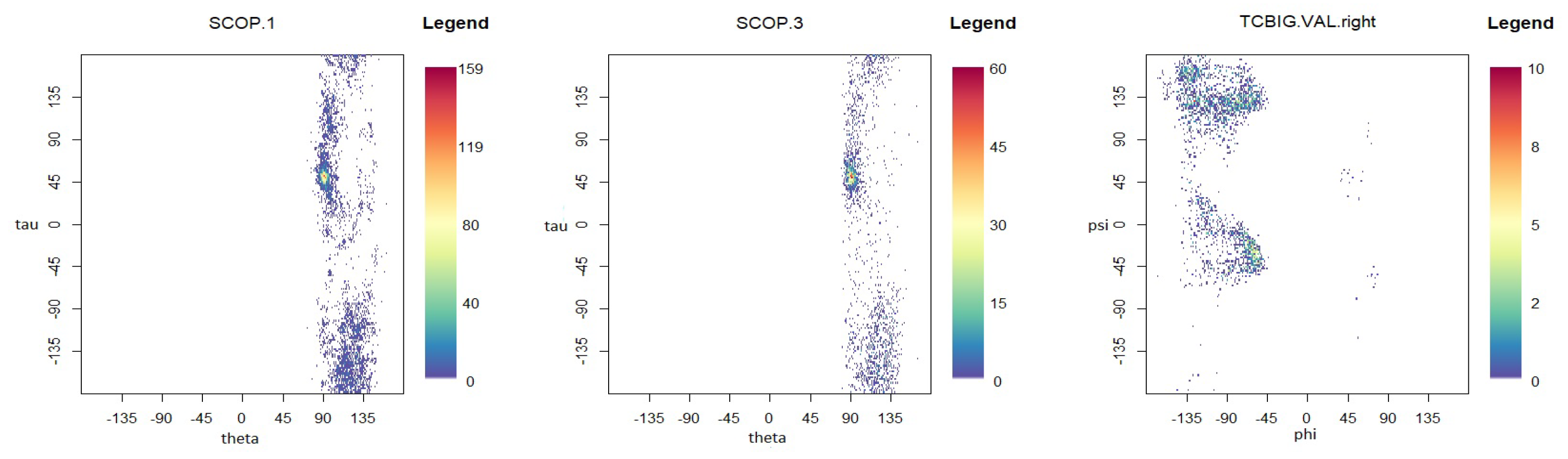
To demonstrate the performance of the proposed models in modelling the dihedral angles and the planar and torsion angles in a protein structure, three datasets are considered, which are available at http://scop.mrc-lmb.cam.ac.uk/scop/. SCOP.1 contains 10,188 planar and torsion angles $(\theta ,\tau )$ (see Figure 1A) for about 63 protein domains that were randomly selected from three remote protein classes in the structural classification of proteins (SCOP). SCOP.3 includes 4607 planar and torsion angles $(\theta ,\tau )$ from approximately 40 protein chains, and the TCBIG.VAL.right set consists of 2673 dihedral angles $(\varphi ,\psi )$ (see Figure 7B) [41]. The Ramachandran plots [1] for each dataset are presented in Figure 8. As can be seen, the datasets are at least bimodal, so bimodal or mixture distributions will be good choices for fitting.

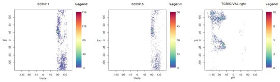
Figure 8. Ramachandran plots for each dataset.

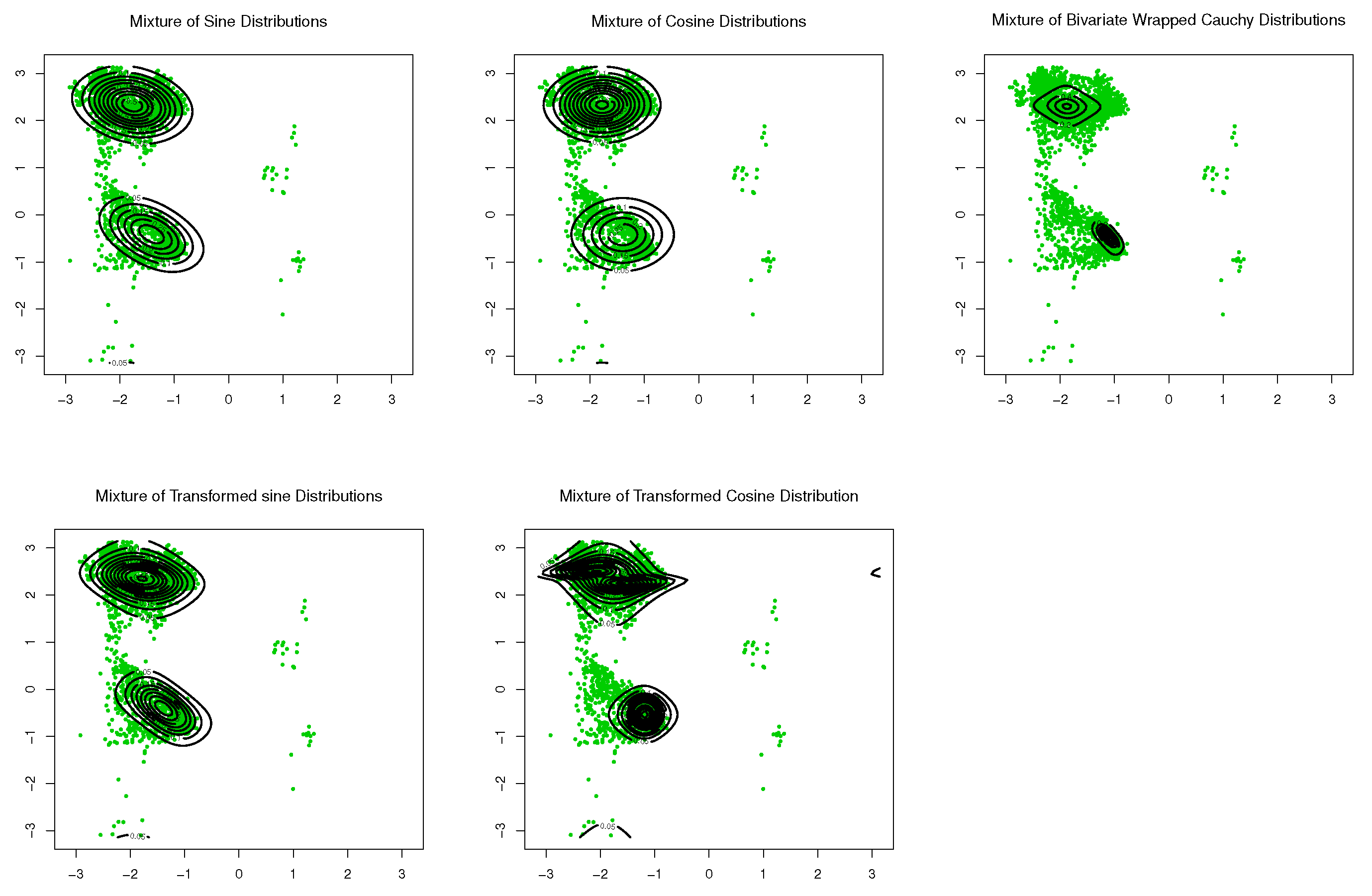
The transformed sine and cosine models in (16) and (10), along with their competitors—the sine model, and a mixture of sine models (see (2); [13]), the cosine model, and a mixture of cosine models (see (4); [14]), and a mixture of bivariate wrapped Cauchy models (see (8); [33])—were fitted to the SCOP.1 and SCOP.3 datasets. A mixture distribution with two components was investigated as follows:

$$g_M({\theta }_1,{\theta }_2)=p{f}_1({\theta }_1,{\theta }_2)+(1-p)f_2({\theta }_1,{\theta }_2)$$

where $p\in [0,1]$ and $f_1(.,.)$ and $f_2(.,.)$ are two toroidal distributions. The estimation of parameters, identifiability, and choosing the number of mixing components and parameters are among the well-known challenges in the application of mixture distributions. Furthermore, when the empirical density of the data is highly asymmetric, it can result in a misleading statistical inference of the parameters [42]. Multimodal distributions, which represent the random behaviour of data with multi-mode presence, can provide better model fitting. This is observed here using the bimodal transformed sine model.

The sine-skewed versions of the aforementioned distributions [24] form part of these evaluations. The results, including the MLEs of parameters, log-likelihood, Akaike information criterion (AIC), and the Bayesian information criterion (BIC), are shown in Table 1 and Table 2. Based on these results, the bimodal transformed sine model in (16) provides the best fit for the data, and its performance is better than that of the mixture models for these datasets. Based on the symmetry test of Ameijeiras-Alonso and Ley in [24] and the values of log-likelihood in Table 1 and Table 2, there is no evidence that rejects the fact that underlying distributions for SCOP.1 and SCOP.3 are pointwise symmetric. The results of the mixture of transformed sine and the mixture of transformed cosine models are not reported in Table 1 and Table 2 because $\widehat{p}\approx 1$. Scatter plots of the data, together with contour plots of the fitted distributions are provided in Figure 9 and Figure 10.

Table 1. Maximum likelihood estimates and corresponding log-likelihood, AIC, and BIC for SCOP.1 ($n=$ 10,188).

Model	$\widehat{\mathit{\rho }}$	${\widehat{\mathit{\kappa }}}_1$	${\widehat{\mathit{\kappa }}}_2$	${\widehat{\mathit{\kappa }}}_3$	${\widehat{\mathit{r}}}_1$	${\widehat{\mathit{r}}}_2$	${\widehat{\mathit{\mu }}}_1$	${\widehat{\mathit{\mu }}}_2$	${\widehat{\mathit{\lambda }}}_1$	${\widehat{\mathit{\lambda }}}_2$	$\widehat{\mathit{p}}$	Log-Likelihood	AIC	BIC
Sine	–	25.2085	0.3679	7.3700	–	–	1.8976	2.4624	–	–	–	$-15,890.80$	31,790.16	31,827.74
[13]
Sine-skewed sine	–	18.8058	0.0852	4.8449	–	–	1.8701	$-3.1415$	0.4051	$-0.3718$	–	$-18,089.71$	36,193.42	36,244.02
[24]
Mixture of sine	–	4.9938	0.4603	2.3512	–	–	2.0560	2.5011	–	–	0.3476
												$-15,719.26$	31,460.22	31,540.04
	–	0.0217	0.0413	$-4.4594$	–	–	1.0912	$-1.8997$	–	–	0.6524
Cosine	–	11.6274	$6.7\times {10}^{-17}$	0.6507	–	–	1.8807	$-0.8652$	–	–	–	$-19,919.04$	39,848.07	39,884.22
[14]
Sine-skewed cosine	–	11.6274	$1.7\times {10}^{-8}$	0.6507	–	–	1.8807	$-0.8651$	$-0.7557$	0.0789	–	$-19,919.04$	39,852.07	39,902.68
[24]
Mixture of cosine	–	9.6015	2.6459	0.0087	–	–	1.7967	0.8676	–	–	0.5266
[14]												$-18,120.09$	36,262.18	36,341.70
	–	8.4761	0.0820	2.3228	–	–	2.1309	0.9647	–	–	0.4734
Mixture of bivariate	$-0.2892$	–	–	–	0.9551	0.5649	1.6129	1.5337	–	–	0.4463
wrapped Cauchy												$-17,099.36$	34,220.72	34,300.24
[33]	$-0.1289$	–	–	–	0.8513	0.5433	2.1128	$-2.6980$	–	–	0.5537
Transformed sine	–	2.1585	0.3489	3.1712	0.6036	0.0131	1.8573	2.4321	–	–	–	−15,558.98	31,131.97	31,182.56
Sine-skewed transformed sine	–	2.1582	0.3487	3.1712	0.6037	0.0131	1.8573	2.4321	$-0.1894$	$0.0556$	–	$-15,558.98$	31,135.97	31,201.02
Transformed cosine	–	4.5122	$1.9\times {10}^{-16}$	2.7905	0.2632	0.4164	1.8806	$-0.6888$	–	–	–	$-16,920.43$	33,854.86	33,905.46
Sine-skewed transformed cosine	–	4.4704	$4.2\times {10}^{-5}$	2.8185	0.2656	0.4228	1.8805	-0.6871	0.6225	$-0.1849$	–	$-16,920.43$	33,858.86	33,923.92

Table 2. Maximum likelihood estimates and corresponding log-likelihood, AIC, and BIC for SCOP.3 ($n=4607$).

Model	$\widehat{\mathit{\rho }}$	${\widehat{\mathit{\kappa }}}_1$	${\widehat{\mathit{\kappa }}}_2$	${\widehat{\mathit{\kappa }}}_3$	${\widehat{\mathit{r}}}_1$	${\widehat{\mathit{r}}}_2$	${\widehat{\mathit{\mu }}}_1$	${\widehat{\mathit{\mu }}}_2$	${\widehat{\mathit{\lambda }}}_1$	${\widehat{\mathit{\lambda }}}_2$	$\widehat{\mathit{p}}$	Log-Likelihood	AIC	BIC
Sine	–	27.0312	0.3243	8.0789	–	–	1.8810	2.4618	–	–	–	$-6970.09$	13,950.18	13,982.36
[13]
Sine-skewed sine	–	26.8304	0.3224	8.0732	–	–	1.8960	2.4724	$-0.4124$	$-0.0159$	–	$-6941.31$	13,896.62	13,941.67
[24]
Mixture of sine	–	7.3842	2.0013	$-6.3567$	–	–	2.0918	$-1.4321$	–	–	0.6632
												$-6893.41$	13,901.15	13,879.61
	–	2.8774	0.0347	$-1.7125$	–	–	1.9306	$-1.1124$	–	–	0.3368
Cosine	–	11.5883	$3.8\times {10}^{-16}$	0.6404	–	–	1.8537	$-0.9851$	–	–	–	$-9028.72$	18,067.45	18,099.62
[14]
Sine-skewed cosine	–	11.5883	$5.0\times {10}^{-9}$	0.6404	–	–	1.8537	$-0.9850$	$-0.0168$	$-0.6387$	–	$-9028.72$	18,071.45	18,116.49
[24]
Mixture of cosine	–	29.9375	1.9210	0.0213	–	–	1.6840	0.8043	–	–	0.5648
[14]												$-6959.76$	13,941.52	14,012.31
	–	17.3302	0.0211	1.9456	–	–	2.0575	0.8866	–	–	0.4352
Mixture of bivariate	$-0.2347$	–	–	–	0.9169	0.5546	1.5969	1.1037	–	–	0.4712
wrapped Cauchy												$-7137.52$	14,297.04	14,367.83
[33]	$-0.1279$	–	–	–	0.8388	0.5100	1.9792	$-2.0869$	–	–	0.5288
Transformed sine	–	3.8755	0.3414	3.6786	0.4950	$1.3\times {10}^{-9}$	1.8589	2.4490	–	–	–	−6905.08	13,824.17	13,869.22
Sine-skewed transformed sine	–	3.8764	0.3415	3.7066	0.4883	$2.6\times {10}^{-8}$	1.8591	2.4491	$-0.1544$	0.0796	–	$-6905.08$	13,828.17	13,886.08
Transformed cosine	–	4.1351	$2.4\times {10}^{-16}$	2.8283	0.2884	0.4183	1.8604	$-0.6560$	–	–	–	$-7567.28$	15,148.56	15,193.61
Sine-skewed transformed cosine	–	4.1350	$6.4\times {10}^{-10}$	2.8283	0.2884	0.4183	1.8604	$-0.6560$	0.6868	$-0.1567$	–	$-7567.27$	15,152.56	15,210.46

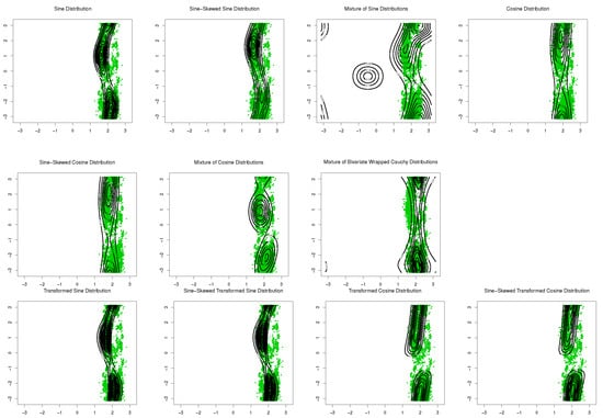
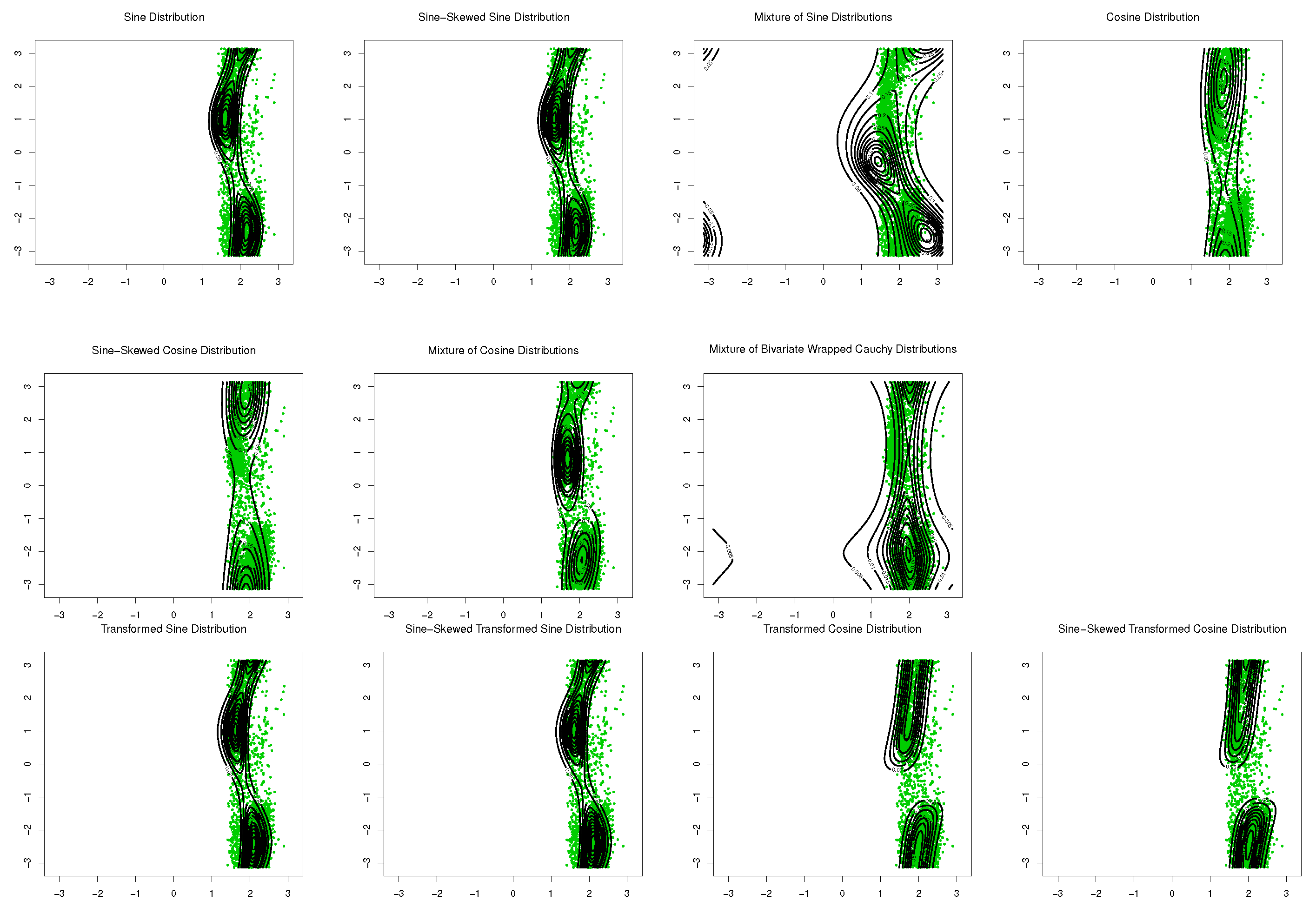
Figure 9. Contour plots of fitted pdfs together with scatter plot for SCOP.1 ($n=$ 10,188). The last row includes the proposed models.

Figure 10. Contour plots of fitted pdfs together with scatter plot for SCOP.3 ($n=4607$). The last row includes the proposed models.

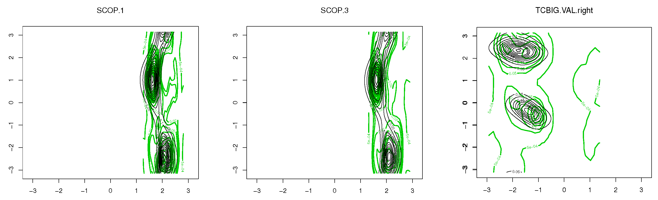
With the last dataset TCBIG.VAL.right, good results are not observed upon application of the single component distributions. Therefore, a mixture model might offer a solution. Subsequently, only mixtures of the aforementioned distributions were considered. For comparison, goodness-of-fit was evaluated for mixtures of distributions from transformed sine and cosine models, and for mixtures of distributions from existing models. The results are listed in Table 3. As can be seen, the mixture of transformed sine models provides the best fitting of the data. Scatter plots of the data and contour plots of the fitted distributions are shown in Figure 11.

Table 3. Maximum likelihood estimates and corresponding log-likelihood, AIC, and BIC for TCBIG.VAL.right ($n=2673$).

Model	$\widehat{\mathit{\rho }}$	${\widehat{\mathit{\kappa }}}_1$	${\widehat{\mathit{\kappa }}}_2$	${\widehat{\mathit{\kappa }}}_3$	${\widehat{\mathit{r}}}_1$	${\widehat{\mathit{r}}}_2$	${\widehat{\mathit{\mu }}}_1$	${\widehat{\mathit{\mu }}}_2$	$\widehat{\mathit{p}}$	Log-Likelihood	AIC	BIC
Mixture of sine	–	4.4364	7.6222	$-1.2187$	–	–	$-1.7736$	2.3336	0.6239
										$-4901.12$	9824.25	9889.04
	–	5.4606	7.7290	$-3.1154$	–	–	$-1.4197$	$-0.4111$	0.3761
Mixture of cosine	–	4.2849	6.1824	$4.6\times {10}^{-6}$	–	–	$-1.4003$	$-0.4191$	0.3787
[14]										$-5005.01$	10,032.03	10,096.82
	–	4.6268	7.8256	$9.1\times {10}^{-6}$	–	–	$-1.7785$	2.3358	0.6213
Mixture of bivariate	$-0.3805$	–	–	–	0.8545	0.8118	$-1.1194$	$-0.4710$	0.3108
wrapped Cauchy										$-5283.42$	10,588.85	10,653.64
[33]	$-0.0294$	–	–	–	0.7038	0.7778	$-1.8772$	2.3037	0.6892
Mixture of transformed sine	–	2.8274	7.3718	$-3.0328$	0.2930	0.0872	$-1.3860$	$-0.4040$	0.3515
										$-4826.80$	9683.61	9771.96
	–	4.0949	1.6545	$-0.7133$	0.02450	0.4387	$-1.7802$	2.3495	0.6485
Mixture of transformed cosine	–	2.3349	9.3385	0.0063	0.4909	0.1287	$-1.1835$	$-0.5358$	0.2645
										$-4882.14$	9794.28	9882.64
–	3.9496	0.0117	0.8886	0.0553	0.8668	$-1.8501$	2.3841	0.7355

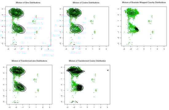
Figure 11. Contour plots of fitted pdfs together with scatter plots for TCBIG.VAL.right ($n=2673$). The last row includes the proposed models.

The kernel density plots of the three datasets and the best-fit models obtained for each dataset are shown in Figure 12. According to the levels of contours in the kernel densities of the data and fitted curves, our proposed models provide an accurate fit.

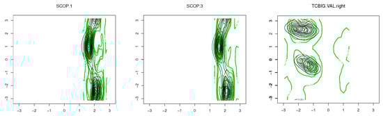
Figure 12. Kernel density plots of the data, and the best-fit models.

6. Simulation Study

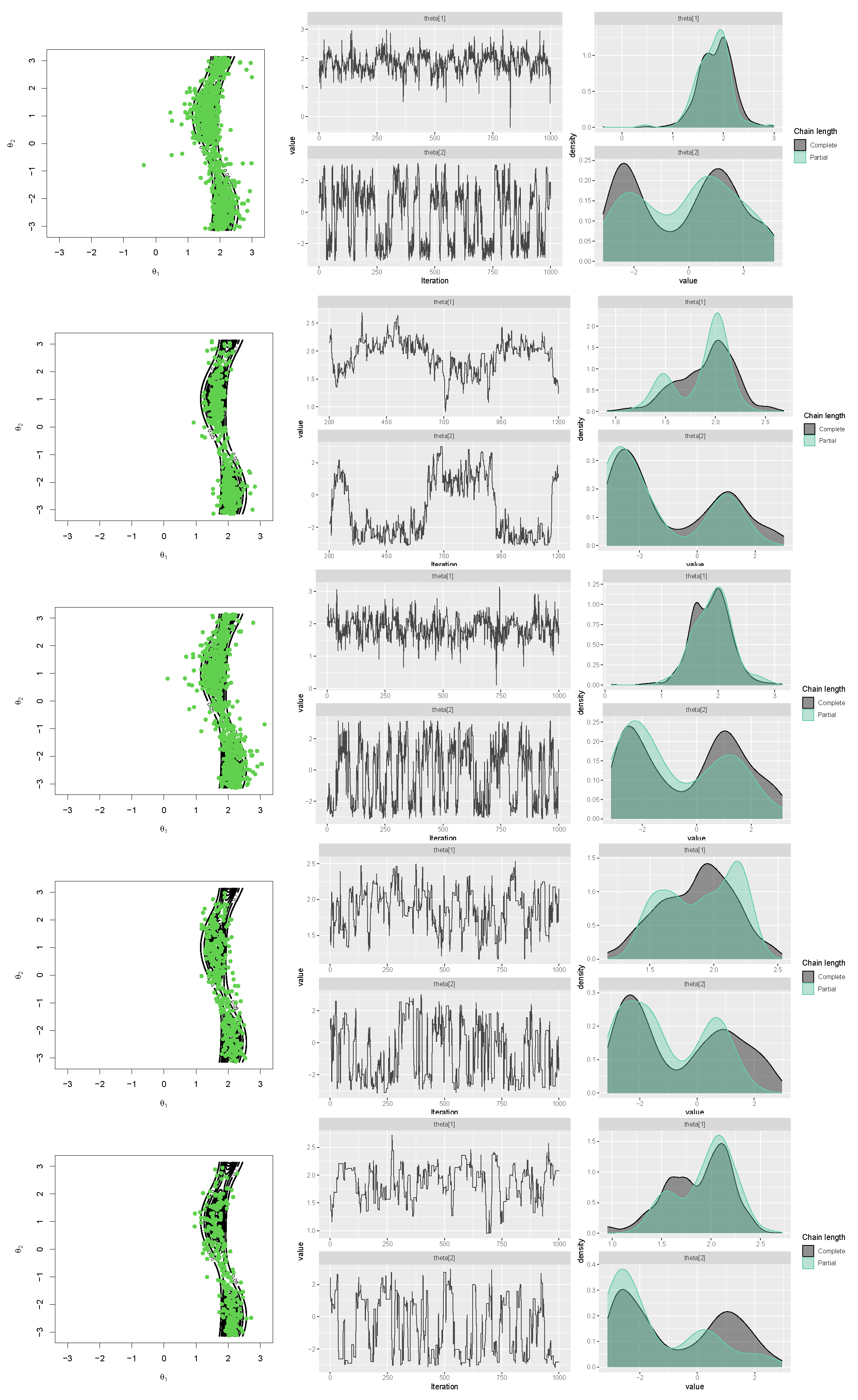
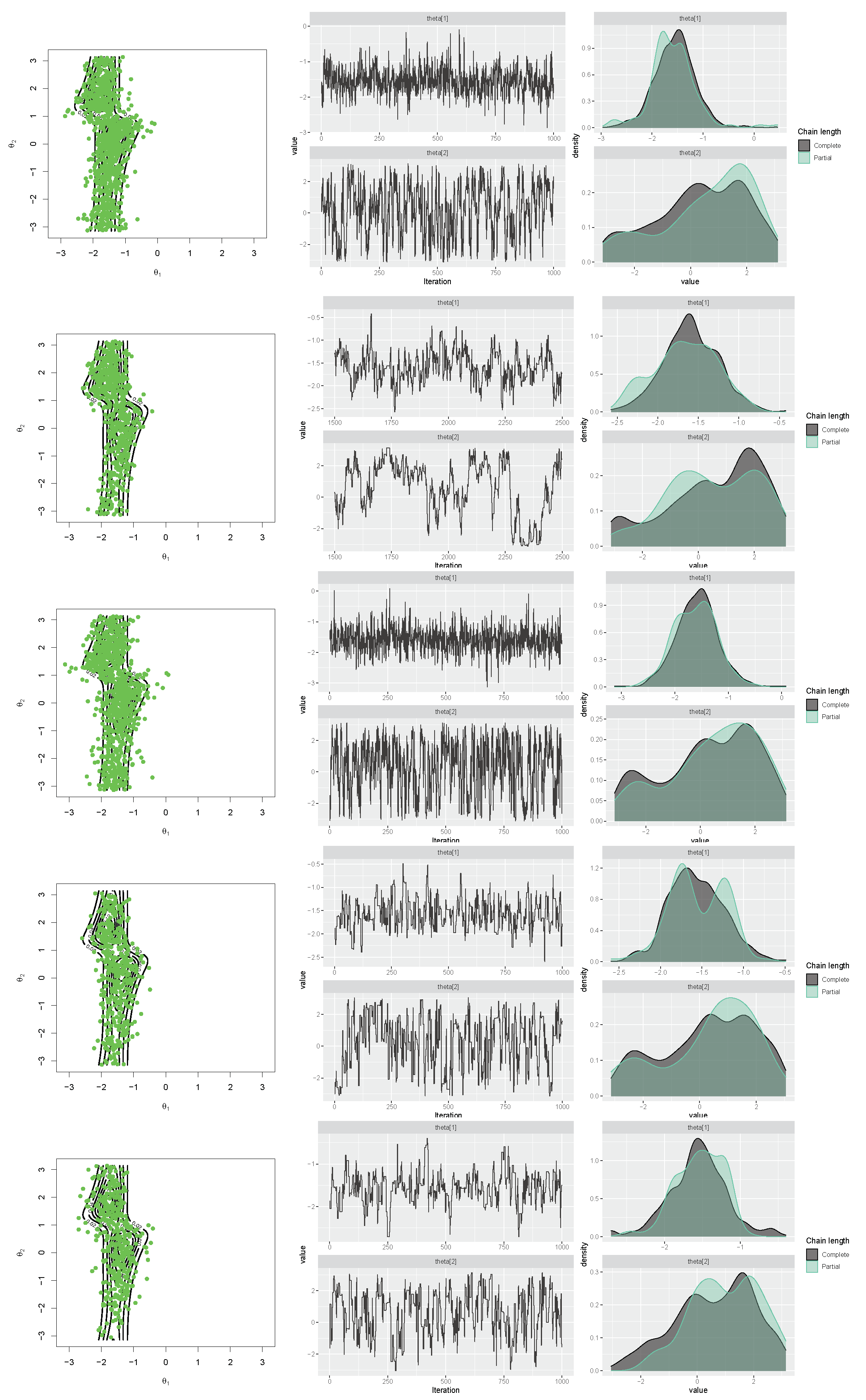
The authors of Ref. [16] explored suitable methods for generating samples from cosine (with positive interaction) and sine models. They found that both Gibbs and rejection sampling approaches performed well, but the latter was more efficient. To simulate a sample from the newly proposed transformed sine and transformed cosine distributions in (16) and (10), four packages in R, which are generally based on rejection sampling, including MCMCpack [43], gibbs.met [44], LearnBayes [45], and MHadaptive [46], were used and the results were compared. These packages are based on Metropolis sampling, random walk Metropolis sampling, Metropolis-Hastings MCMC sampling, and Gibbs sampling with Metropolis steps. First, a sample of size $n=1000$ was generated with each package from the transformed sine model in (16), with the parameters ${\kappa }_1=2.1585$, ${\kappa }_2=0.3489$, ${\kappa }_3=3.1712$, $r_1=0.6036$, $r_2=0.0131$, ${\mu }_1=1.8573$, and ${\mu }_2=2.4321$ (the best-fit model for the SCOP.1 dataset in the previous section). The results, including scatter plots of simulated samples with contour plots of the distribution, trace plots, and compare-partial plots [47], which use the last 10 percent of the chain, are shown in Figure 13. The runtime of each method is shown in Figure 14 (left) for a sample size of $n=100$ [48] (system: Intel(R) Core(TM) i7-8550U CPU @ 1.80 GHz RAM 8.00 GB). Second, the MLE of the parameters and bias and the mean squared error (MSE) of the estimates were calculated for each method using the Monte Carlo method, with 500 replications and n = 1,001,000. The results are listed in Table 4.

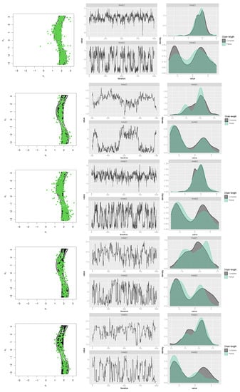
Figure 13. Scatter, trace, and compare-partial plots of the simulated data from the transformed sine model using “gibbs_met” in the “gibbs.met” package (first row), “MCMCmetrop1R” in the “MCMCpack” package (second row), “met_gaussian” in the “gibbs.met” package (third row), “Metro_Hastings” in the “MHadaptive” package (fourth row), and “rwmetrop” in the “LearnBayes” package (fifth row).

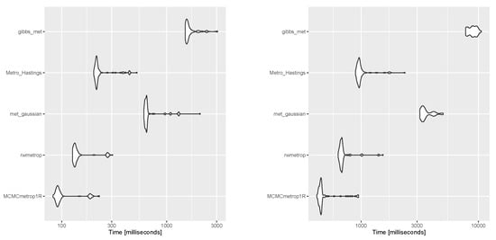
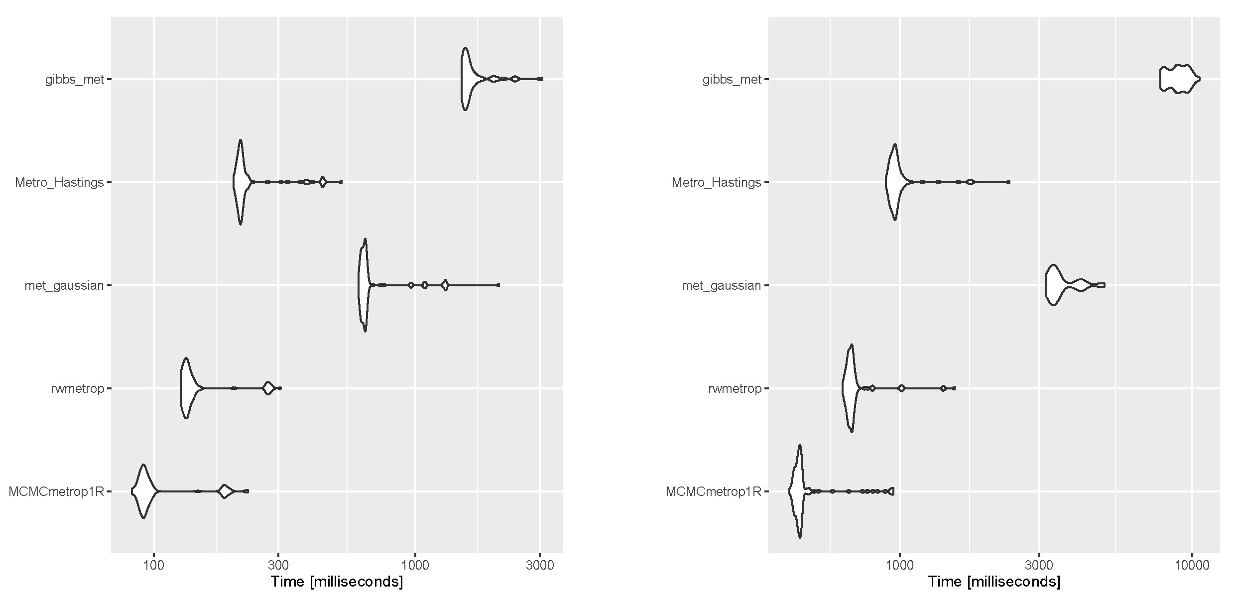
Figure 14. Execution times for generating a sample size of $n=100$ from a transformed sine model (left) and a transformed cosine model (right) for each method.

Table 4. Maximum likelihood estimates of parameters and bias, and the MSE of the estimates for the simulated data obtained from each method.

Method	Distribution	n		${\mathit{\kappa }}_1$	${\mathit{\kappa }}_2$	${\mathit{\kappa }}_3$	${\mathit{r}}_1$	${\mathit{r}}_2$	${\mathit{\mu }}_1$	${\mathit{\mu }}_2$
			MLE	1.8450	0.2876	2.8360	0.6001	0.0063	1.7744	2.6177
		$n=100$	Bias	$-0.0542$	$-0.1932$	$-0.1531$	$-0.0089$	$-0.0521$	$-0.0815$	0.1185
			MSE	0.0879	0.0921	0.1864	0.0083	0.0044	0.0087	0.0344
	Transformed sine
			MLE	2.1311	0.2649	3.1546	0.6243	0.0395	1.8491	2.4263
		$n=1000$	Bias	$-0.0298$	$-0.0900$	$-0.0135$	0.0142	0.0130	$-0.0018$	$-0.0046$
			MSE	0.0527	0.0588	0.0002	0.0018	0.0008	0.0005	$2.5\times {10}^{-5}$
MCMCmetrop1R
			MLE	3.7753	0.5985	1.5693	0.2564	0.4660	$-1.4684$	1.0937
		$n=100$	Bias	$-0.1137$	$-0.0572$	$-0.1022$	0.0143	$-0.0376$	0.0957	0.0421
			MSE	0.0998	0.0932	0.1007	0.0028	0.0116	0.0135	0.0275
	Transformed cosine
			MLE	4.0693	0.6305	1.8210	0.2546	0.5557	$-1.5613$	1.0116
		$n=1000$	Bias	0.0758	$-0.0319$	0.0305	0.0241	0.0329	0.0037	0.0238
			MSE	0.0065	0.0426	0.0085	0.0007	0.0014	0.0007	0.0011
			MLE	1.8186	0.2260	3.2619	0.6444	0.0359	1.8815	2.6027
		$n=100$	Bias	$-0.2337$	$-0.0867$	0.3837	0.0398	0.0205	0.0370	0.1006
			MSE	0.1094	0.0350	0.0726	0.0016	0.0406	0.0022	0.0291
	Transformed sine
			MLE	1.9735	0.3887	3.1546	0.6204	0.0159	1.8701	2.4270
		$n=1000$	Bias	0.0979	0.0360	$-0.0165$	0.0131	0.0046	0.0129	$-0.0046$
			MSE	0.0340	0.0482	0.0003	0.0004	0.0001	0.0005	$2.1\times {10}^{-5}$
rwmetrop
			MLE	3.8086	0.5397	1.4956	0.1726	0.5929	$-1.5746$	1.0417
		$n=100$	Bias	$-0.0984$	$-0.0940$	$-0.2954$	$-0.0512$	0.0883	$-0.0115$	0.0524
			MSE	0.0902	0.0893	0.1003	0.0033	0.0088	0.0009	0.0037
	Transformed cosine
			MLE	3.9139	0.7320	1.8188	0.2546	0.4667	$-1.5766$	0.9962
		$n=1000$	Bias	$-0.0758$	0.0703	$0.0166$	0.0241	$-0.0386$	$-0.0095$	0.0084
			MSE	0.0056	0.0674	0.0007	0.0013	0.0014	0.0007	0.0018
			MLE	2.5400	0.4480	3.1322	0.6963	0.1087	1.8321	2.3133
		$n=100$	Bias	0.3469	0.0904	$-0.0328$	0.0837	0.0916	$-0.0294$	$-0.0908$
			MSE	0.1773	0.0583	0.0117	0.0092	0.0091	0.0009	0.0141
	Transformed sine
			MLE	1.9022	0.2894	3.3403	0.6649	0.0016	1.8619	2.3822
		$n=1000$	Bias	$-0.2223$	$-0.0658$	0.1137	0.0607	$-0.0123$	0.0042	$-0.0481$
			MSE	0.1268	0.0042	0.0286	0.0043	0.0025	$2.1\times {10}^{-5}$	0.0024
met_gaussian
			MLE	3.4389	0.5409	1.4373	0.2530	0.5214	$-1.5411$	1.0526
		$n=100$	Bias	$-0.3642$	$-0.1187$	$-0.2970$	0.0143	0.0113	0.0210	0.0623
			MSE	0.1927	0.0993	0.1251	0.0853	0.0082	0.0005	0.0041
	Transformed cosine
			MLE	3.6491	0.5341	1.6260	0.2420	0.5134	$-1.5720$	1.0158
		$n=1000$	Bias	$-0.2978$	$-0.1049$	$-0.0999$	0.0195	0.0027	$-0.0105$	0.0126
			MSE	0.1214	0.0915	0.0875	0.0019	0.0032	0.0005	0.0024
			MLE	2.1465	0.2728	2.6713	0.6912	0.0010	1.8107	2.2024
		$n=100$	Bias	$-0.0197$	$-0.0784$	$-0.4598$	0.0856	$0.0770$	$-0.0603$	$-0.1029$
			MSE	0.0434	0.0883	0.2498	0.0073	0.0059	0.0046	0.0527
	Transformed sine
			MLE	2.1657	0.2743	3.2124	0.5813	0.0762	1.8487	2.4826
		$n=1000$	Bias	0.0362	$-0.0456$	0.0433	$-0.0262$	0.0531	$-0.0081$	0.0404
			MSE	0.0246	0.0556	0.0027	0.0011	0.0039	$7.3\times {10}^{-5}$	0.0025
Metro_Hastings
			MLE	3.8290	0.5903	2.0419	0.2857	0.5753	$-1.5434$	0.8373
		$n=100$	Bias	$-0.1600$	$-0.0582$	0.2407	0.0577	0.0709	0.0172	$-0.1202$
			MSE	0.1998	0.0944	0.1208	0.0061	0.0059	0.0006	0.0266
	Transformed cosine
			MLE	3.8936	0.6747	1.5822	0.2775	0.4859	$-1.5676$	0.9935
		$n=1000$	Bias	$-0.0961$	0.0298	$-0.2317$	0.0470	$-0.0196$	$-0.0025$	0.0057
			MSE	0.0091	0.0847	0.0829	0.0030	0.0003	0.0002	0.0051
			MLE	2.2340	0.2728	2.8277	0.6198	0.1398	1.8437	2.1688
		$n=100$	Bias	0.0712	$-0.0784$	$-0.3884$	0.0143	0.1220	$-0.0129$	$-0.2598$
			MSE	0.1171	0.0583	0.1179	0.0092	0.0160	0.0003	0.0692
	Transformed sine
			MLE	2.1901	0.3555	3.1760	0.6016	0.0156	1.8573	2.4342
		$n=1000$	Bias	0.0315	0.0066	0.0048	$-0.0020$	0.0024	$6.1\times {10}^{-5}$	0.0021
			MSE	0.0963	0.0221	0.0464	0.0008	0.0003	$1.7\times {10}^{-5}$	0.0018
gibbs_met
			MLE	3.6123	0.5732	1.5193	0.2006	0.5852	$-1.5886$	0.8808
		$n=100$	Bias	$-0.2842$	$-0.0853$	$-0.2717$	$-0.0276$	0.0869	$-0.0238$	$-0.0758$
			MSE	0.1419	0.0893	0.1067	0.0082	0.0087	0.0005	0.0187
	Transformed cosine
			MLE	3.6322	0.5978	1.7613	0.2626	0.5793	$-1.5685$	0.9668
		$n=1000$	Bias	$-0.2568$	$-0.0653$	$-0.0232$	0.0221	0.0648	$-0.0034$	$-0.0209$
			MSE	0.0915	0.0726	0.0008	0.0031	0.0074	0.0002	0.0046

Similarly, for the transformed cosine model in (10) with parameters ${\kappa }_1=3.9891$, ${\kappa }_2=0.6532$, ${\kappa }_3=1.7911$, $r_1=0.2305$, $r_2=0.5046$, ${\mu }_1=-1.5651$, and ${\mu }_2=0.9878$, the aforementioned R packages were applied, first to generate a sample size of $n=1000$. The results, including scatter plots of simulated samples with contour plots of the distribution, trace plots, and compare-partial plots [47], are shown in Figure 15. The runtime of each method is presented in Figure 14 (right) for a sample size of n = 100 [48]. Then, the MLE of the parameters and bias and the MSE of the estimates were calculated for each method using the Monte Carlo method, with 500 replications and n = 100,1000. The results are listed in Table 4, which support the performance of the selected approach for obtaining the MLEs of parameters. As shown in Figure 14, the MCMCmetrop1R is the highest-speed method, and gibbs_met is the lowest-speed method. According to the results in Table 4, rejection sampling provides accurate results. Gibbs sampling with Metropolis steps (gibbs_met) is also precise despite the low speed. With increasing n, bias and MSE decrease.

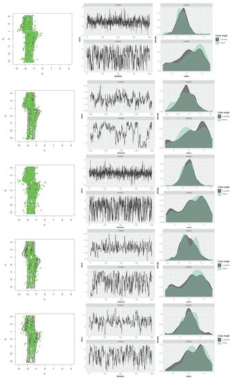
Figure 15. Scatter, trace, and compare-partial plots of the simulated data from the transformed cosine model using “gibbs_met” in the “gibbs.met” package (first row), “MCMCmetrop1R” in the “MCMCpack” package (second row), “met_gaussian” in the “gibbs.met” package (third row), “Metro_Hastings” in the “MHadaptive” package (fourth row), and “rwmetrop” in the “LearnBayes” package (fifth row).

7. Conclusions

In MCMC protein sampling for predicting the 3D structure, when the proposal distribution is closer to the stationary distribution, the results are more accurate. Therefore, a suitable proposal distribution can be defined using the angles and bond lengths observed in natural proteins. Statistical distributions for modelling protein dihedral angles can be used as proposal distributions for MCMC protein sampling. We gave a brief overview of existing symmetric models that formed the basis of the proposed models in this paper ((2) and (4)). In addition, new Möbius transformation-induced toroidal distributions, together with skewed versions, were developed in this study as alternatives to proposal distributions for the MCMC sampling of proteins. We demonstrated their performance with three protein datasets of toroidal nature and graphically illustrated their flexible behaviour. The AIC and BIC confirmed the better performance of our proposed models in comparison with the existing models. These newly proposed models even outperformed mixtures of well-known models for modelling toroidal data. In comparison with the existing toroidal models, these proposed models reflect the protein structural information better and should be incorporated into proposal distributions. Lastly, to meet the need for sampling of proposal distribution in the MCMC algorithm, suitable methods for generating samples from these new models were explored using different types of the Metropolis sampling. In the future, one can investigate the performance of the Möbius transformation to obtain new cylindrical distributions.

Appendix A.1. Proof of Proposition 1

When $r_1,r_2\to 0$, pdf (10) tends to the cosine distribution, which for large values of ${\kappa }_1$ and ${\kappa }_2$ is concentrated near 0. Suppose ${\mu }_1={\mu }_2=0$ (without loss of generality), according to Theorem 1 in [14] and using Taylor expansions, $({\mathsf{\Theta }}_1,{\mathsf{\Theta }}_2)\sim N_2(0,\mathsf{\Sigma })$, where ${\mathsf{\Sigma }}^{-1}=\left(\begin{array}{cc}{\kappa }_1-{\kappa }_3& {\kappa }_3\\ {\kappa }_3& {\kappa }_2-{\kappa }_3\end{array}\right)$, with ${\kappa }_3\le \frac{{\kappa }_1{\kappa }_2}{{\kappa }_1+{\kappa }_2}$.

Appendix A.2. Proof of Corollary 1

Without loss of generality, we consider ${\mu }_1=0$. According to (12), we conclude that:

$$\begin{array}{cc}\hfill \frac{f_{{\mathsf{\Theta }}_1}^{\prime }\left({\theta }_1\right)}{f_{{\mathsf{\Theta }}_1}\left({\theta }_1\right)}& =\{\frac{-2r_1}{(1+r_1^2-2r_{1}cos{\theta }_1)}+\frac{{\kappa }_2{\kappa }_3{(1-r_1^2)}^{2}A\left(h\left({\theta }_1\right)\right)}{h\left({\theta }_1\right){(1+r_1^2-2r_{1}cos{\theta }_1)}^2}\hfill \\ & -\frac{{\kappa }_1{(1-r_1^2)}^2}{{(1+r_1^2-2r_{1}cos{\theta }_1)}^2}\}sin{\theta }_1\hfill \\ & =g\left({\theta }_1\right)sin{\theta }_1.\hfill \end{array}$$

(A1)

In (A1), if ${\kappa }_3<0$, then $g\left({\theta }_1\right)<0$. Therefore, for ${\theta }_1\in [0,\pi )$, $f_{{\mathsf{\Theta }}_1}^{\prime }\left({\theta }_1\right)<0$, and for ${\theta }_1\in [-\pi ,0)$, $f_{{\mathsf{\Theta }}_1}^{\prime }\left({\theta }_1\right)\ge 0$. Thus, $f_{{\mathsf{\Theta }}_1}\left({\theta }_1\right)$ is increasing in $[-\pi ,0)$ and decreases from 0 to $\pi$. In addition, $f_{{\mathsf{\Theta }}_1}\left({\theta }_1\right)=f_{{\mathsf{\Theta }}_1}(-{\theta }_1)$, which means that $f_{{\mathsf{\Theta }}_1}\left({\theta }_1\right)$ is symmetric around 0; thus, for ${\kappa }_3<0$, $f_{{\mathsf{\Theta }}_1}\left({\theta }_1\right)$ is unimodal. If ${\kappa }_3>0$, $h\left({\theta }_1\right)$ decreases from $-\pi$ to 0 and increases from 0 to $\pi$, and $h\left(0\right)=\mid {\kappa }_2-{\kappa }_3\mid$ and $h(-\pi )={\kappa }_2+{\kappa }_3$. From Lemma 1 in Singh et al. (2002), $A\left(t\right)/t$ is a decreasing function of t; therefore, $A\left(h\left({\theta }_1\right)\right)/h\left({\theta }_1\right)$ is increasing in $[-\pi ,0)$ and decreases from 0 to $\pi$. It can be concluded that $g\left({\theta }_1\right)$ is decreasing in $[0,\pi )$ and increasing in $[-\pi ,0)$; hence, if $-2r_1+{\kappa }_2{\kappa }_3\frac{A(\mid {\kappa }_2-{\kappa }_3\mid )}{\mid {\kappa }_2-{\kappa }_3\mid }\frac{{(1-r_1^2)}^2}{{(1-r_1)}^2}-{\kappa }_1\frac{{(1-r_1^2)}^2}{{(1-r_1)}^2}<0$, then $f_{{\mathsf{\Theta }}_1}^{\prime }\left({\theta }_1\right)\ge 0$ for ${\theta }_1\in [-\pi ,0)$ and $f_{{\mathsf{\Theta }}_1}^{\prime }\left({\theta }_1\right)<0$ for ${\theta }_1\in [0,\pi )$; which means that $f_{{\mathsf{\Theta }}_1}\left({\theta }_1\right)$ is unimodal. If $-2r_1+{\kappa }_2{\kappa }_3\frac{A(\mid {\kappa }_2-{\kappa }_3\mid )}{\mid {\kappa }_2-{\kappa }_3\mid }\frac{{(1-r_1^2)}^2}{{(1-r_1)}^2}-{\kappa }_1\frac{{(1-r_1^2)}^2}{{(1-r_1)}^2}>0$ and $-2r_1+{\kappa }_2{\kappa }_3\frac{A({\kappa }_2+{\kappa }_3)}{{\kappa }_2+{\kappa }_3}\frac{{(1-r_1^2)}^2}{{(1+r_1)}^2}-{\kappa }_1\frac{{(1-r_1^2)}^2}{{(1+r_1)}^2}\le 0$, then $f_{{\mathsf{\Theta }}_1}\left({\theta }_1\right)$ is first increasing and then decreasing in $[-\pi ,0)$, which means that $f_{{\mathsf{\Theta }}_1}\left({\theta }_1\right)$ is bimodal. A more detailed proof is provided by the authors upon request.

Appendix A.3. Proof of Corollary 2

Suppose ${\mu }_1=0$ (without loss of generality). According to (18), the following result can be obtained:

$$\begin{array}{cc}\frac{f_{{\mathsf{\Theta }}_1}^{\prime }\left({\theta }_1\right)}{f_{{\mathsf{\Theta }}_1}\left({\theta }_1\right)}& =\{\frac{-2r_1}{(1+r_1^2-2r_{1}cos{\theta }_1)}-\frac{{\kappa }_1{(1-r_1^2)}^2}{{(1+r_1^2-2r_{1}cos{\theta }_1)}^2}+\frac{{\kappa }_3^2{(1-r_1^2)}^{2}A\left(h\left({\theta }_1\right)\right)}{h\left({\theta }_1\right){(1+r_1^2-2r_{1}cos{\theta }_1)}^4}\hfill \\ & \times \left(({(1+r_1^2)}^2+4r_1^2)cos{\theta }_1-4r_1(1+r_1^2){cos}^2{\theta }_1-2r_1(1+r_1^2){sin}^2{\theta }_1\right)\}sin{\theta }_1\hfill \\ & =g\left({\theta }_1\right)sin{\theta }_1.\hfill \end{array}$$

(A2)

In (A2), if $cos{\theta }_1\le 0$, then $g\left({\theta }_1\right)<0$ and the sign of (A2) depends on the sign of $sin{\theta }_1$. Hence, for ${\theta }_1\in (-\pi ,-\pi /2]$, $f_{{\mathsf{\Theta }}_1}^{\prime }\left({\theta }_1\right)<0$ and for ${\theta }_1\in [\pi /2,\pi ]$, $f_{{\mathsf{\Theta }}_1}^{\prime }\left({\theta }_1\right)\ge 0$. Thus, $f_{{\mathsf{\Theta }}_1}\left({\theta }_1\right)$ is increasing in $(-\pi ,-\pi /2]$ and decreasing from $\pi /2$ to $\pi$. In addition, $f_{{\mathsf{\Theta }}_1}\left({\theta }_1\right)=f_{{\mathsf{\Theta }}_1}(-{\theta }_1)$, which means that $f_{{\mathsf{\Theta }}_1}\left({\theta }_1\right)$ is symmetric around 0; therefore, $f_{{\mathsf{\Theta }}_1}\left({\theta }_1\right)$ is unimodal. For $\theta \in [0,\pi /2]$, $h\left({\theta }_1\right)$ is an increasing function of ${\theta }_1$, and according to Lemma 1 in [13], $A\left(h\left({\theta }_1\right)\right)/h\left({\theta }_1\right)$ is a decreasing function of ${\theta }_1$. We can conclude that if $-2r{(1-r_1)}^2-{\kappa }_1{(1-r_1^2)}^2+{\kappa }_3^2{(1-r_1^2)}^2\frac{A\left({\kappa }_2\right)}{{\kappa }_2}<0$, then $f_{{\mathsf{\Theta }}_1}\left({\theta }_1\right)$ is a decreasing function from 0 to $\pi /2$, and because $f_{{\mathsf{\Theta }}_1}\left({\theta }_1\right)$ is symmetric around 0, it increases from $-\pi /2$ to 0. If $-2r{(1-r_1)}^2-{\kappa }_1{(1-r_1^2)}^2+{\kappa }_3^2{(1-r_1^2)}^2\frac{A\left({\kappa }_2\right)}{{\kappa }_2}>0$, then $f_{{\mathsf{\Theta }}_1}\left({\theta }_1\right)$ first increases and then decreases in $[0,\pi /2]$ and $[-\pi /2,0]$ (because it is symmetric around 0), which states that $f_{{\mathsf{\Theta }}_1}\left({\theta }_1\right)$ is bimodal.

References

- Ramachandran, G.T.; Sasisekharan, V. Conformation of polypeptides and proteins. Adv. Protein Chem. 1968, 23, 283–437. [Google Scholar]
- Holley, L.H.; Karplus, M. Protein secondary structure prediction with a neural network. Proc. Natl. Acad. Sci. USA 1989, 86, 152–156. [Google Scholar] [CrossRef] [Green Version]
- Metropolis, N.; Rosenbluth, A.W.; Rosenbluth, M.N.; Teller, A.H.; Teller, E. Equation of state calculations by fast computing machines. J. Chem. Phys. 1953, 21, 1087–1092. [Google Scholar] [CrossRef] [Green Version]
- Hastings, W.K. Monte Carlo sampling methods using Markov chains and their applications. Biometrika 1970, 57, 97–109. [Google Scholar] [CrossRef]
- Irbäck, A.; Mohanty, S. PROFASI: A Monte Carlo simulation package for protein folding and aggregation. J. Comput. Chem. 2006, 27, 1548–1555. [Google Scholar] [CrossRef]
- Jones, D.T. Successful ab initio prediction of the tertiary structure of NK-lysin using multiple sequences and recognized supersecondary structural motifs. Proteins Struct. Funct. Bioinform. 1997, 29, 185–191. [Google Scholar] [CrossRef]
- Jones, T.A.; Thirup, S. Using known substructures in protein model building and crystallography. Embo J. 1986, 5, 819–822. [Google Scholar] [CrossRef]
- Simons, K.T.; Kooperberg, C.; Huang, E.; Baker, D. Assembly of protein tertiary structures from fragments with similar local sequences using simulated annealing and Bayesian scoring functions. J. Mol. Biol. 1997, 268, 209–225. [Google Scholar] [CrossRef] [Green Version]
- Ley, C.; Verdebout, T. Applied Directional Statistics: Modern Methods and Case Studies; CRC Press: Boca Raton, FL, USA, 2018. [Google Scholar]
- Ley, C.; Verdebout, T. Modern Directional Statistics; CRC Press: Boca Raton, FL, USA, 2017. [Google Scholar]
- Mardia, K.V. Statistics of directional data. J. R. Stat. Soc. Ser. B (Methodol.) 1975, 37, 349–371. [Google Scholar] [CrossRef]
- Rivest, L.P. A distribution for dependent unit vectors. Commun. Stat.-Theory Methods 1988, 17, 461–483. [Google Scholar] [CrossRef]
- Singh, H.; Hnizdo, V.; Demchuk, E. Probabilistic model for two dependent circular variables. Biometrika 2002, 89, 719–723. [Google Scholar] [CrossRef]
- Mardia, K.V.; Taylor, C.C.; Subramaniam, G.K. Protein bioinformatics and mixtures of bivariate von-Mises distributions for angular data. Biometrics 2007, 63, 505–512. [Google Scholar] [CrossRef]
- Kent, J.T.; Mardia, K.V.; Taylor, C.C. Modelling strategies for bivariate circular data. In Proceedings of the Leeds Annual Statistical Research Conference; The Art and Science of Statistical Bioinformatics, Leeds University Press: Leeds, UK, 2008; pp. 70–73. [Google Scholar]
- Mardia, K.V.; Frellsen, J. Statistics of bivariate von Mises distributions. In Bayesian Methods in Structural Bioinformatics; Springer: Berlin/Heidelberg, Germany, 2012; pp. 159–178. [Google Scholar]
- Mardia, K.V.; Hughes, G.; Taylor, C.C.; Singh, H. A multivariate von Mises distribution with applications to bioinformatics. Can. J. Stat. 2008, 36, 99–109. [Google Scholar] [CrossRef]
- Wehrly, T.E.; Johnson, R.A. Bivariate models for dependence of angular observations and a related Markov process. Biometrika 1980, 67, 255–256. [Google Scholar] [CrossRef]
- Jones, M.C.; Pewsey, A.; Kato, S. On a class of circulas: Copulas for circular distributions. Ann. Inst. Stat. Math. 2015, 67, 843–862. [Google Scholar] [CrossRef]
- Fernández-Durán, J.J. Models for circular–linear and circular–circular data constructed from circular distributions based on nonnegative trigonometric sums. Biometrics 2007, 63, 579–585. [Google Scholar] [CrossRef]
- García-Portugués, E.; Crujeiras, R.M.; González-Manteiga, W. Exploring wind direction and SO2 concentration by circular–linear density estimation. Stoch. Environ. Res. Risk Assess. 2013, 27, 1055–1067. [Google Scholar] [CrossRef] [Green Version]
- Pewsey, A.; García-Portugués, E. Recent advances in directional statistics. TEST 2021, 30, 1–58. [Google Scholar] [CrossRef]
- Di Marzio, M.; Panzera, A.; Taylor, C.C. Kernel density estimation on the torus. J. Stat. Plan. Inference 2011, 141, 2156–2173. [Google Scholar] [CrossRef] [Green Version]
- Ameijeiras-Alonso, J.; Ley, C. Sine-skewed toroidal distributions and their application in protein bioinformatics. Biostatistics 2020. Available online: https://doi.org/10.1093/biostatistics/kxaa039 (accessed on 20 January 2021). [CrossRef]
- Kato, S.; Shimizu, K.; Shieh, G.S. A circular–circular regression model. Stat. Sin. 2008, 18, 633–645. [Google Scholar]
- Shieh, G.S.; Johnson, R.A. Inferences based on a bivariate distribution with von-Mises marginals. Ann. Inst. Stat. Math. 2005, 57, 789–802. [Google Scholar] [CrossRef]
- Shieh, G.S.; Zheng, S.; Johnson, R.A.; Chang, Y.F.; Shimizu, K.; Wang, C.C.; Tang, S.L. Modeling and comparing the organization of circular genomes. Bioinformatics 2011, 27, 912–918. [Google Scholar] [CrossRef]
- Liu, D.; Peddada, S.D.; Li, L.; Weinberg, C.R. Phase analysis of circadian-related genes in two tissues. BMC Bioinform. 2006, 7, 87. [Google Scholar] [CrossRef] [PubMed] [Green Version]
- Downs, T.D.; Mardia, K.V. Circular regression. Biometrika 2002, 89, 683–697. [Google Scholar] [CrossRef]
- Jones, M.C. The Möbius distribution on the disc. Ann. Inst. Stat. Math. 2004, 56, 733–742. [Google Scholar] [CrossRef]
- Kato, S.; Jones, M.C. A family of distributions on the circle with links to, and applications arising from, Möbius transformation. J. Am. Stat. Assoc. 2010, 105, 249–262. [Google Scholar] [CrossRef] [Green Version]
- Wang, M.Z.; Shimizu, K. On applying Möbius transformation to cardioid random variables. Stat. Methodol. 2012, 9, 604–614. [Google Scholar] [CrossRef]
- Kato, S.; Pewsey, A. A Möbius transformation-induced distribution on the torus. Biometrika 2015, 102, 359–370. [Google Scholar] [CrossRef]
- Kato, S. A distribution for a pair of unit vectors generated by Brownian motion. Bernoulli 2009, 15, 898–921. [Google Scholar] [CrossRef]
- Kato, S.; McCullagh, P. Some properties of a Cauchy family on the sphere derived from the Möbius transformation. Bernoulli 2020, 26, 3224–3248. [Google Scholar] [CrossRef]
- McCullagh, P. Möbius transformation and Cauchy parameter estimation. Ann. Stat. 1996, 24, 787–808. [Google Scholar] [CrossRef]
- Abe, T.; Pewsey, A. Sine-skewed circular distributions. Stat. Pap. 2011, 52, 683–707. [Google Scholar] [CrossRef]
- Mullen, K.; Ardia, D.; Gil, D.L.; Windover, D.; Cline, J. DEoptim: An R package for global optimization by differential evolution. J. Stat. Softw. 2011, 40, 1–26. [Google Scholar] [CrossRef] [Green Version]
- Storn, R.; Price, K. Differential evolution-a simple and efficient heuristic for global optimization over continuous spaces. J. Glob. Optim. 1997, 11, 341–359. [Google Scholar] [CrossRef]
- Price, K.; Storn, R.M.; Lampinen, J.A. Differential Evolution: A Practical Approach to Global Optimization; Springer: Berlin/Heidelberg, Germany, 2006. [Google Scholar]
- Najibi, S.M.; Maadooliat, M.; Zhou, L.; Huang, J.Z.; Gao, X. Protein structure classification and loop modeling using multiple Ramachandran distributions. Comput. Struct. Biotechnol. J. 2017, 15, 243–254. [Google Scholar] [CrossRef] [PubMed] [Green Version]
- Moghimbeygi, M.; Golalizadeh, M. Spherical logistic distribution. Commun. Math. Stat. 2020, 8, 151–166. [Google Scholar] [CrossRef]
- Martin, A.D.; Quinn, K.M.; Park, J.H.; Park, M.J.H. MCMCpack: Markov Chain Monte Carlo (MCMC) Package; Version 1.5-0; R Package: Vienna, Austria, 2020; Available online: https://cran.r-project.org/web/packages/MCMCpack/index.html (accessed on 25 August 2020).
- Li, L. gibbs.met: Naive Gibbs Sampling with Metropolis Steps; Version 1.1-3; R Package: Vienna, Austria, 2015; Available online: https://cran.r-project.org/web/packages/gibbs.met/index.html (accessed on 25 August 2020).
- Albert, J. LearnBayes: Functions for Learning Bayesian Inference; Version 2.15.1; R Package: Vienna, Austria, 2018; Available online: https://cran.r-project.org/web/packages/LearnBayes/index.html (accessed on 25 August 2020).
- Chivers, C.; Chivers, M.C. MHadaptive: General Markov Chain Monte Carlo for Bayesian Inference Using Adaptive Metropolis-Hastings Sampling; Version 1.1-8; R Package: Vienna, Austria, 2015; Available online: https://cran.r-project.org/web/packages/MHadaptive/index.html (accessed on 25 August 2020).
- Fernández-i-Marın, X. ggmcmc: Analysis of MCMC samples and Bayesian inference. J. Stat. Softw. 2016, 70, 1–20. [Google Scholar] [CrossRef] [Green Version]
- Mersmann, O. Microbenchmark: Accurate Timing Functions; Version 1.4-7; R Package: Vienna, Austria, 2019; Available online: https://www.rdocumentation.org/packages/microbenchmark/versions/1.4-7/topics/microbenchmark (accessed on 25 August 2020).
Publisher’s Note: MDPI stays neutral with regard to jurisdictional claims in published maps and institutional affiliations. |
© 2021 by the authors. Licensee MDPI, Basel, Switzerland. This article is an open access article distributed under the terms and conditions of the Creative Commons Attribution (CC BY) license (https://creativecommons.org/licenses/by/4.0/).