Web-Based Tool for Algebraic Modeling and Mathematical Optimization

Abstract

In this article, we present a new open-source tool for algebraic modeling and mathematical optimization. We begin by distilling the main gaps within the existing algebraic modeling languages and tools (varying performance, limited cross-compatibility, complex syntax, and different solver, feature, and problem type support). Later, we propose a state-of-the-art web-based tool (WebAML and Optimization System) for algebraic modeling languages and mathematical optimization. The tool does not require specific algebraic language knowledge, allows solving problems using different solvers, and utilizes the best characteristics of existing algebraic modeling languages. We also provide clear extension points and ideas on how we could further improve such a tool.

1. Introduction

It is common to routinely solve real-world problems using modern optimization tools (e.g., [1,2,3,4,5,6]). These tools combine a mathematical model with an appropriate solution algorithm (e.g., [4,5,7,8,9,10,11,12,13]) to solve the problem at hand. Thus, the way mathematical models are formulated is critical for the impact of mathematical optimization in real life. Examples of real-life problems include production and shipment by firms, investment planning, macroeconomics stabilization, water distribution networks, oil refineries, petrochemical plants, applied general equilibrium, international trade of aluminum and copper, and many more [14]. Algebraic modeling languages (AMLs) are declarative mathematical optimization modeling languages, which bridge the gap between model formulation and the proper solution technique [2]. They facilitate the formulation of a mathematical model as a human-readable set of equations. Moreover, they do not require specifying how the described model should be solved or what mathematical optimization solver should be used. Models written in an AML are known for the high degree of similarity to the mathematical formulation. Such an algebraic design approach allows practitioners without specific programming or modeling knowledge to be efficient in describing the problems to be solved.

In general, AMLs are advanced software that provides a central link between an optimization model’s mathematical concept and the complex mathematical optimization solvers used to determine optimal solutions. Typically, AML software automatically reads a model and the data generates an instance and transfers it to a solver in the required format [15].

From the late 1970s, numerous AMLs were created (e.g., AMPL [16], GAMS [17]) and are still actively developed and used today. Lately, new open-source competitors to the traditional AMLs started to appear (e.g., Pyomo [18,19], JuMP [20,21]). Thus, we deem it important to identify, compare, and evaluate the most important characteristics of modeling systems and algebraic modeling languages.

Some comparisons of AMLs are made based on questionnaires sent out by the vendors [22]. At the same time, in our previous research [23], we have conducted an extensive theoretical and experimental analysis of the characteristics of the most prominent AMLs (AMPL, GAMS, JuMP, and Pyomo) and the modeling systems supporting them. In a theoretical comparison, we evaluated how the reviewed modern AMLs match the current needs of practitioners. While performing the experimental analysis, we used a purpose-built test model library to perform extensive performance and presolving benchmarks.

We feel the need to continue research by further distilling the main gaps within the existing AMLs and proposing both a more generalized modeling language and an open-source-based tool combining the best characteristics of the existing AMLs. While a suggestion for using LATEX as a foundation for the AML tool by Triantafyllidis and Papageorgiou [24] already exists, we believe another, more user-friendly alternative can be provided.

The contributions of this paper are the following:

• It identifies the differences amongst the most prominent algebraic modeling languages for mathematical optimization, which make it challenging for practitioners to learn and use it.
• It proposes concepts for a universal algebraic modeling language aimed to simplify mathematical modeling and optimization. Thus, making it easier to learn and be taught in a mathematics classroom and still making it suitable for a usual practitioner once faced with a need for solving real-life mathematical optimization problems.
• It provides the prototype of the universal mathematical optimization system (WebAML and Optimization Ecosystem), implementing the proposed concepts and combining the best characteristics of the most prominent AMLs.

The remainder of the paper is organized as follows: Section 2 presents an overview on how the characteristics of the most prominent algebraic modeling languages differ and what challenges it poses for a practitioner. Section 3 defines concepts of the universal algebraic modeling language (WebAML) and describes a prototype of the optimization ecosystem supporting it. Section 4 compares the proposed way of algebraic modeling with classical ones and comments on the extensibility of the proposed language and prototype. Finally, Section 5 concludes our work.

2. Materials and Methods

First, we need to identify the differences which make the most prominent AMLs difficult for practitioners to learn and use. We start by examining the results published in our previous research [23] and using datasets provided as part of it [25]. We continue to compare AMPL, GAMS, JuMP, and Pyomo, which were identified as the most prominent ones in our previous research. To compare the practical aspects of the algebraic modeling, we have chosen to use an example of the classical transportation problem by Dantzig, G. B. [26], which can be stated mathematically as seen in Listing 1.

This is a linear programming problem in which the objective function is to minimize the cost of transportation subject to demand and supply constraints. The transportation problem applies to situations where a single commodity is transported from various sources of supply (origins) to different demands (destinations).

Let there be m sources of supply $s_1,s_2,\dots ,s_m$ having $a_i$ (i = $1,2,\dots ,m$) units of supplies, respectively, to be transported among n destinations $d_1,d_2,\dots ,d_n$ with $b_j$ (j = $1,2,\dots ,n$) units of requirements, respectively.

Let $c_{ij}$ be the cost for shipping one unit of the commodity from source i to destination j for each route. Suppose $x_{ij}$ represents the units shipped per route from source i to destination j. In that case, the problem is determining the transportation schedule that minimizes the total cost of satisfying the supply and demand conditions.

Listing 1. The classical transportation problem by Dantzig, G. B.  [26].
Minimize:
	$$\sum _{i=1}^m\sum _{j=1}^n{c}_{ij}{x}_{ij}$$
Subject to:
	$$\sum _{j=1}^n{x}_{ij}\le a_i, \mathrm{for}i=1,2,\dots ,m(\mathrm{supply}\mathrm{constraints})$$
	$$\sum _{i=1}^m{x}_{ij}\ge b_j, \mathrm{for}j=1,2,\dots ,n(\mathrm{demand}\mathrm{constraints})$$
	$$x_{ij}\ge 0, \mathrm{for}\mathrm{all}i=1,2,\dots ,m\mathrm{and}j=1,2,\dots ,n$$

2.1. General Features

Based on the information available on the vendors’ websites of the discussed AMLs, the general features are provided in

Table 1. General features of AMPL, GAMS, Pyomo, and JuMP software packages.

General Feature	AMPL	GAMS	JuMP	Pyomo
Operating system	Win/Mac/Unix	Win/Mac/Unix	Win/Mac/Unix	Win/Mac/Unix
First released	1985	1978	2017	2008
User interface	GUI (Textual)	GUI (Textual)	Command line	Command line
License	Commercial	Commercial	Free	Free

. We can observe that none of them have a full-fledged graphical user interface (GUI) to do the modeling. AMPL and GAMS provide a simple GUI for writing a textual model code and running standard commands. Pyomo and JuMP do not have any graphical interface at all.

They all support the three major operating systems (Windows, Unix, and Mac). Therefore, the usage is relatively the same independent of what operating system or hardware the modeler is using. However, it requires local installation, and thus access to the same physical machine is needed.

AMPL and GAMS are commercial tools with academic licenses starting at USD 500 and the basic commercial license from USD 4000. However, adding more solvers might easily double the price. JuMP and Pyomo are open source and distributed for free, though the solvers have to be procured separately.

2.2. Syntax

The syntax to describe the problems for different AMLs is a noticeable difference to explore. Fragniere and Gondzio [2] state that the algebraic design approach used in AMLs should allow practitioners without specific programming or modeling knowledge to be efficient in describing the problems to be solved. However, observing constraints of the same problem defined in Listing 2, we can conclude that it does require some programming knowledge to use AMLs such as Pyomo and JuMP, and it is also not a straightforward process to switch between different AMLs. Exploring more complex language structures (e.g., calculated parameters, suffixes) showcases even more differences between the syntax of AMLs and complexity for practitioners to learn multiple of them.

Listing 2. The objective function and constraints of the transportation problem [26] expressed in AMPL, GAMS, Pyomo, and JuMP syntax.

# AMPL minimize cost: sum{i in I, j in J} c[i,j] ∗ x[i,j]; s.t. supply{i in I}: sum{j in J} x[i,j] <= a[i]; s.t. demand{j in J}: sum{i in I} x[i,j] >= b[j];

# GAMS cost..      z =e= sum((i,j), c(i,j)∗x(i,j)); supply(i).. sum(j, x(i,j)) =l= a(i); demand(j).. sum(i, x(i,j)) =g= b(j);

# Pyomo def objective_rule (model):    return sum(model.c[i,j]∗model.x[i,j] for i in model.i for j in model. j) model.objective = Objective (rule=objective_rule, sense=minimize) def supply_rule (model, i):    return sum(model.x[i,j] for j in model. j) <= model.a [i] model.supply = Constraint (model.i, rule=supply_rule) def demand_rule (model, j):    return sum(model.x[i,j] for i in model. i) >= model.b [j] model.demand = Constraint (model.j, rule=demand_rule)

# JuMP @objective (model, Min, sum(cost_f[i, j] ∗ trans[i,j]     for i in 1:length(ORIG), j in 1: length(DEST))) @constraint (model, [i in 1: length(ORIG)],     sum(trans[i, j] for j in 1: length(DEST)) <= supply [i]) @constraint (model, [j in 1: length(DEST)],     sum(trans[i, j] for i in 1: length(ORIG)) >= demand [j])

2.3. Compatibility

The compatibility between AMLs from a tooling perspective is also scarce. GAMS Convert [27] is the only tool (commercial) capable of converting between different AMLs. However, the conversion results in a scalar model being produced where the original model structure is lost. An example of a GAMS Convert-generated scalar model in Pyomo format can be seen in Listing 3. Once compared to the model in an original Pyomo format, as seen in Listing 4, the scalar model becomes more difficult to read, understand, and extend.

Listing 3. The classical transportation problem [26] expressed in a Pyomo scalar format.

from pyomo.environ import ∗

model = m = ConcreteModel ()

m.x1 = Var(within=Reals,bounds=(0,None),initialize=0) m.x2 = Var(within=Reals,bounds=(0,None),initialize=0) m.x3 = Var(within=Reals,bounds=(0,None),initialize=0) m.x4 = Var(within=Reals,bounds=(0,None),initialize=0) m.x5 = Var(within=Reals,bounds=(0,None),initialize=0) m.x6 = Var(within=Reals,bounds=(0,None),initialize=0)

m.obj = Objective(expr=   0.225∗m.x1 + 0.153∗m.x2             + 0.162∗m.x3 + 0.225∗m.x4 + 0.162∗m.x5 + 0.126∗m.x6, sense=minimize) m.c2 = Constraint(expr=   m.x1 + m.x2 + m.x3 <= 350) m.c3 = Constraint(expr=   m.x4 + m.x5 + m.x6 <= 600) m.c4 = Constraint(expr=   m.x1 + m.x4 >= 325) m.c5 = Constraint(expr=   m.x2 + m.x5 >= 300) m.c6 = Constraint(expr=   m.x3 + m.x6 >= 275)

Furthermore, during our recent benchmarks [25], we have identified a few flaws of the GAMS Convert tool. Around 3% of models available in the GAMS library were converted to AMPL, Pyomo, and JuMP with syntax errors, making them unsolvable. Most of the Pyomo errors were caused by an incorrect GAMS Convert tool behavior where the definition of the Suffix primitive uses AMPL but not Pyomo semantics. Similar issues were observed in some of the JuMP models.

Listing 4. The classical transportation problem [26] expressed in a Pyomo original format.

from pyomo.environ import ∗ model = ConcreteModel () model.i = Set(initialize=[’seattle’,’san-diego’]) model.j = Set(initialize=[’new-york’,’chicago’, ’topeka’]) model.a = Param(model.i, initialize={’seattle’:350,’san-diego’:600}) model.b = Param(model.j, initialize={’new-york’:325,’chicago’:300,’topeka’:275}) dtab = {      (’seattle’,  ’new-york’)  : 2.5,      (’seattle’,  ’chicago’)   : 1.7,      (’seattle’,  ’topeka’)    : 1.8,      (’san-diego’,’new-york’) : 2.5,      (’san-diego’,’chicago’)  : 1.8,      (’san-diego’,’topeka’)   : 1.4,      } model.d = Param(model.i, model.j, initialize=dtab) model.f = Param(initialize=90) def c_init(model, i, j):      return model.f ∗ model.d[i,j] / 1000 model.c = Param(model.i, model.j, initialize=c_init) model.x = Var(model.i, model.j, bounds=(0.0,None)) def supply_rule(model, i):      return sum(model.x[i,j] for j in model.j) <= model.a[i] model.supply = Constraint(model.i, rule=supply_rule) def demand_rule(model, j):      return sum(model.x[i,j] for i in model.i) >= model.b[j] model.demand = Constraint(model.j, rule=demand_rule) def objective_rule(model):      return sum(model.c[i,j]∗model.x[i,j] for i in model.i for j in model.j) model.objective = Objective(rule=objective_rule, sense=minimize)

2.4. Solvers

Solvers are an essential part of what a modern AML offers. They implement appropriate solution algorithms to solve the problem at hand. Some solvers are distributed together with AMLs, while others can be purchased separately.

Since the “No Free Lunch Theorems for Optimization” [28] states that for certain types of mathematical problems, the computational cost of finding a solution, averaged over all problems in the class, is the same for any solution method. Thus, no single universal solver for all problem types can exist. This is why in

Table 2. The number of solvers supported by AMLs grouped by the problem type.

Type	AMPL	GAMS	JuMP	Pyomo
Global	4	9	2	1
LP	17	21	9	10
MCP	1	5	1	1
MINLP	6	15	3	6
MIP	14	16	6	8
MIQCP	5	20	3	4
NLP	19	17	7	10
QCP	9	21	6	6
Total	47	35	14	25

, we provide an overview of the solvers supported by different AMLs grouped by problem types. As solvers usually support several types of optimization problems, the last row reflects the total number of unique solvers.

The quality of the algorithms implemented by the solvers is also important. In our research, we have identified AMPL and GAMS as the ones providing the most extensive set of state-of-the-art solvers for various types of mathematical optimization problems. The list of supported solvers is continuously updated and growing [29,30]. We believe that some solvers might be more significant since having support for multiple problem types makes it appealing for practitioners. However, being universal does not guarantee the best performance. Thus, practitioners might prefer more specialized but also more efficient solvers.

AMPL comes with the majority of solvers bundled in a standard package. However, it should not be confused that the solvers supported by AMPL are the exact solvers supported by other AMLs. We can get into a situation where a specific problem needs a solver, which is only available through the one and only AML. This would require the modeler to define the model in a given AML, and it must be known upfront. It is not always the case in real-life situations where the nature of the problem is not fully understood until it has been defined in a specific AML and attempted to be solved.

2.5. Performance

Performance becomes essential once we start to solve complex real-life problems. Models tend to grow in size and input data amount. Thus, we must focus on the solvers’ performances, i.e., solution time, and consider the potential savings in a model instance generation phase. Our benchmark results in Figure 1 [23] show significant model instance generation time variation between different AMLs. It is important to note that while AMPL is a clear top performer, open-source counterparts have varying results within different problem types. Thus, choosing the right AML for a concrete problem type would impact performance.

2.6. Presolving

Presolving, a feature supported by very few AMLs, attempts to reduce the problem size or determine the problem to be unfeasible even before sending it to the solver. Out of the benchmarked AMLs, only AMPL supports presolving. Our research observed that an AMPL presolver managed to simplify models in 52.8% of the cases, out of which five times it determined that the problem solution is not feasible, thus not requiring to call the solver. On average, once applied, the AMPL presolver managed to reduce the model size by removing 18.42% of constraints and 10.73% of variables.

The benchmark seen in

Table 3. Benchmark of AMPL presolve impact on solving. Sample models were solved with a Gurobi solver, and the solver’s presolve function turned off while keeping AMPL presolver on.

	Iteration-Wise	Time-Wise	Iteration-Wise (%)	Time-Wise (%)
Positive	33	44	54.10%	72.13%
Neutral	10	0	16.39%	0.00%
Negative	18	17	29.51%	27.87%

was made to test the impact of the AMPL presolve on solution time. The results were positive, allowing us to conclude that the presolver is an efficient way to simplify larger problems leading to improved solution finding performance once invoking a solver with an already reduced problem model instance. Moreover, the ability to determine infeasible models can help modelers in the problem definition process debug and find errors in the model definition.

2.7. Parallelism

Parallelism is a feature we have not explored in our previous research, but it is significant for solving real-life mathematical optimization problems. We can identify three prominent use cases of parallelism within AMLs.

First, it is the parallelism in a problem-solving phase implemented by the solver algorithms. There is the opportunity to use parallel computations to aid in the search for (global) solutions, typically in a nonconvex (or discrete) setting. Mathematical optimization algorithms have also utilized building blocks, most prominently decomposition and parallel linear algebra techniques, to exploit the computational power of high-performance machines [31].

Secondly, in some applications, optimization of a collection of problems is required where each problem is structurally the same. Still, some or all of the data defining the instance is updated [32]. Solving such collections of problems could benefit from the single initiation of the base model instance, updating the base model instance with specific scenario information and solving the scenarios in parallel.

Lastly, truly large-scale problems may require parallel processing for the solution of the problem and during the model generation phase [33]. For this, we need an AML that facilitates the modeling of the problem structure and can utilize problem structure in the parallel model generation.

Our work focuses on the last two types of parallelism within AMLs since the first one is implemented by the solvers and not by the AMLs themselves.

Table 4. Support for parallel scenario solving and parallel model generation in AMPL, GAMS, Pyomo, and JuMP.

Type of Parallelism	AMPL	GAMS	JuMP	Pyomo
Scenario solving	Preampl [34]	GUSS/GRID [31]	StructJuMP [35]	Pyro/PH [36]
Model generation	PSMG [37]	.stage/GDX [38]	StructJuMP [35]	N/A

provides a brief overview of how specific AMLs can implement the two types of parallelism in which we are interested. It is worth noting that in none of the AMLs, parallel scenario solving or parallel model generation is implemented by default. The tools or techniques cited in Table 4 are provided by the scientific society, not the vendors themselves.

2.8. Summary

Summarizing all of the observations about differences within AMLs described so far, we find the following:

• Practitioners must learn the specific syntax of a given AML, which is coupled to a specific modeling environment. Practitioners are not flexible to reuse the knowledge and simplify work;
• Very limited cross-compatibility between different AMLs makes it practically impossible to transfer the model from one AML to another automatically. This might result in vendor lock-in—choosing to stay with a specific AML due to the increased cost of switching;
• Different AMLs support different solvers, so, in some scenarios, practitioners might have a solver available in another AML than the model is written and will not be able to utilize it;
• Different AMLs have different levels of support for various model types. Since in the beginning it is not always clear what type of problem we are dealing with, it is risky to choose AML, which might not be supported;
• As identified in our practical benchmark, AML performance differs significantly between modeling environments and model types. It is beneficial to be flexible in choosing the best one for large models;
• Varying support for additional capabilities such as presolving or parallel solving.

This leads us to believe that while there are a few powerful modeling environments and AMLs, neither provide a complete feature set required for the efficient and intuitive modeling of mathematical optimization problems.

To address the identified gaps, we propose developing a "universal” AML and a tool supporting it, which would benefit from the best characteristics of all of the existing AMLs. We strongly believe that an open-source and web-based approach will make it much more accessible for a wider audience, will not require local installations, and will utilize cloud computing power. Thus, we are suggesting a web-based tool which:

• Does not require syntax knowledge of any specific AML. Everything can be done via a guided graphical user interface;
• Internally combines and utilizes the best characteristics of different AMLs. Thus, it is capable of converting between different AMLs;
• Is designed for enabling presolving and parallel solving in the future;
• Provides a framework for other contributors to extend it (e.g., feature to choose the best solver based on the model type automatically).

3. Results

We have worked on two main building blocks supporting the vision of the universal algebraic modeling system. The first one is a formal language capable of capturing problem characteristics, which we call WebAML. The second one is a prototype of the tool allowing us to build a model using the WebAML language and solve it using the underlying AMLs. We have scoped the prototype to support three key operations—load the model from a file, solve the model, and export the model to a file. Currently, our prototype supports three AMLs: AMPL, GAMS, and Pyomo. All of the results and code base is available in our WebAML GitHub repository [39], which is structured as follows:

• The webaml-schema directory contains the WebAML language definitions and transportation problem example;
• The webaml-c4model directory contains an architecture model for a reference implementation of WebAML and Optimization System;
• The webaml-backend directory contains Java-based backend services supporting WebAML;
• The webaml-frontend directory contains a single-page front-end application for building and manipulating WebAML models.

3.1. WebAML Language

Once deciding on how to design and define WebAML language for structuring, validating, and capturing the mathematical optimization model logic, we have taken into account the following criteria:

• Models will be built using a graphical user interface. Thus, there is no need to have a short and straightforward syntax;
• Model has to be strictly typed and well structured to allow converting it to the syntax of other AMLs;
• Model will be used on the Web. Thus, the data interchange format should be lightweight, open, standardized, and well adopted on the Web.

Based on the criteria above, we have decided to choose JSON [40] as a lightweight data-interchange format and JSON Schema [41] as a metadata format to describe and validate our WebAML data format. Most programming languages widely support JSON, which is human-readable, and have a small metadata footprint compared to other formalized formats such as, e.g., XML. Using JSON Schema creates additional value since tooling to generate OpenAPI-based (the OpenAPI: language-agnostic interface to RESTful APIs; https://swagger.io/specification (accessed on 17 September 2021)) services from JSON Schema can simplify the development of a prototype while supporting more accessible updates once the WebAML language format evolves.

We also had to choose how to capture the mathematical equations needed to define constraints in the model. Here, we have chosen to use a well-known language, such as LATEX, instead of its less-adopted counterparts, such as ASCII Math (AsciiMath: an easy-to-write markup language for mathematics; http://asciimath.org (accessed on 17 September 2021)). This was dictated by both widespread knowledge of LATEX in academic society and the existence of libraries capable of tokenizing LATEX formulas (LATEX.js: JavaScript LATEX to HTML5 translator; https://latex.js.org (accessed on 17 September 2021)) and displaying them nicely on the Web using W3C MathML [42] standard.

A detailed structure of a WebAML model is defined in the JSON Schema file called webaml.schema.json (accessed on 10 October 2021), available on our GitHub repository. At the same time, a summary of the basic components is provided in

Table 5. Basic components of WebAML language.

Component	Type	Comment
Set	Single-dimensional	String and number data types supported
Table	Two-dimensional	Number data type supported
Parameter	Scalar	Fixed value
	Indexed	Can be calculated
Variable	Continuous	Upper/lower bound supported
	Binary	-
	Integer	Upper/lower bound supported
Constraint	Simple	For a single variable
	Indexed	Defined over a set
Objective	Minimize	Single objective only
	Maximize	Single objective only

.

As seen in Table 5, at the moment, we have limited our language to support only the basic features. Thus, no syntactic sugar is maintained (e.g., aliases), and only single-dimensional sets and two-dimensional arrays are supported. Features such as indexing over partial sets are also not supported. However, our JSON Schema is defined in a flexible manner. If the tooling working with the WebAML language supported more features, it would be easy to extend the WebAML language by introducing new enumerated type values to the schema definition.

In Listing 5, we demonstrate how the same constraints of the transportation problem provided in Listing 2 look in WebAML syntax. While being more verbose, we can observe that it is also much more structured, thus making it easier to write code capable of interpreting and converting it to different formats.

Listing 5. Constraints of transportation problem [26] expressed in WebAML syntax.

"constraints": [        {          "name": "supply",          "type": "INDEXED",          "indexes": ["i"],          "value": "\\sum_j x_{ij} \\leq a_i",          "description": "Observe supply limit at plant"         },         {          "name": "demand",          "type": "INDEXED",          "indexes": ["j"],          "value": "\\sum_i x_{ij} \\geq b_j",          "description": "Satisfy demand at market"        }     ],     "objectives": [        {          "name": "cost",          "type": "MINIMIZE",          "value": "\\sum_i \\sum_j c_{ij} ∗ x_{ij}",          "description": "MINIMIZE transportation cost"        }     ]

3.2. Prototype of WebAML Optimization System

As identified in our earlier findings, we were set to build an extendable, open-source, web-based prototype combining the best characteristics of the underlying AMLs. In Figure 2, we provide the system architecture landscape viewpoint for this prototype of the universal WebAML Optimization System using C4 architecture model (The C4 model for visualizing the software architecture; https://c4model.com (accessed on 17 September 2021)) notation. A more detailed system component diagram can be seen in Figure A1. All of the code is provided on our WebAML GitHub repository [39].

We can observe that the WebAML modeling and mathematical optimization tool acts as an orchestrator that allows the AML modeler to build the model, convert it to a specific AML format, and send it for solving via local solvers or remote solving in the NEOS Server platform. This way, we are not building any new solving capabilities, instead of relying and building on top of the best features provided by the most prominent AMLs.

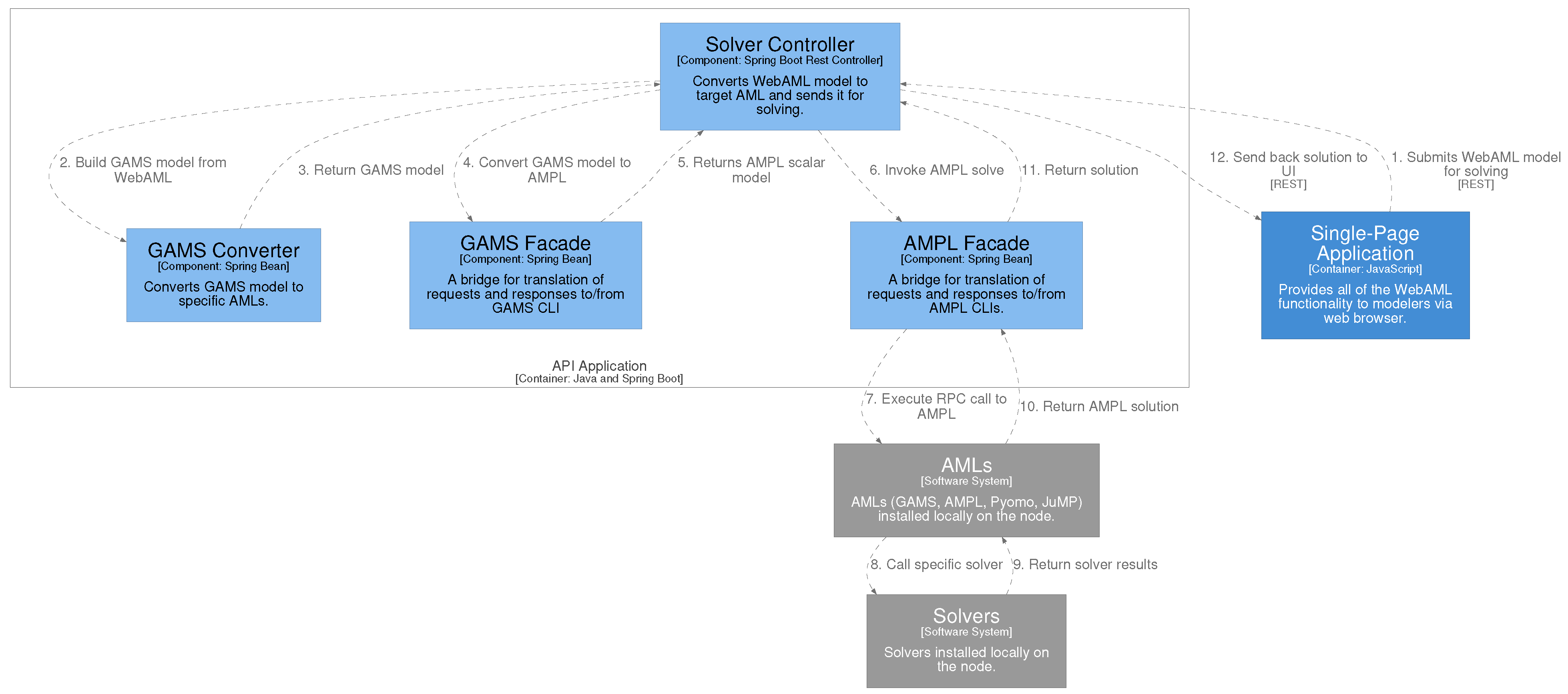
We are also proposing to utilize the GAMS Convert tool to support an even wider variety of AMLs. Adding the support for a new AML that GAMS Convert already supports is as easy as converting WebAML to GAMS (which already has native support in our prototype) and then using GAMS Convert to convert to any other target AML. We have shown how such an approach can work in the AMPL and Pyomo converters provided in the prototype. A detailed description of how such a solution works while using AMPL as an underlying AML is provided in Figure A2.

When implementing the prototype, we have chosen to split our front-end and back-end parts of the prototype into:

• Client-side single page, React.js (React: A JavaScript library for building user interfaces; https://reactjs.org (accessed on 17 September 2021)), the base application responsible for guiding the user while building a WebAML model;
• Back-end application implemented using Spring Boot (Spring Boot: a framework for building stand-alone, production-grade Spring-based applications; https://spring.io/projects/spring-boot (accessed on 17 September 2021)) capable of parsing and converting WebAML language to other AMLs and communicating with underlying AMLs for solving the model.

This approach allows us to leverage the strength of modern browser support for JSON and JSON Schema standards and offload the building of a WebAML model to the client-side, thus reducing the load on the back-end services. The back-end also benefits from the fact that WebAML is a JSON-based language and can quickly validate incoming requests based on the standard JSON Schema while generating OpenAPI-based service contracts using it.

Our prototype provides a simple yet straightforward and guided graphical user interface for constructing a WebAML model. Examples of how the constraints of the transportation problem [26] are displayed in our user interface can be seen in Section 4.1. Since we decided to use LATEX for storing mathematical equations, we also included an on-the-fly MathML-based visualizer of LATEX equations. We believe this helps validate the mathematical expressions and guides nonsavvy LATEX practitioners in the modeling process.

4. Discussion

We believe that in this research, we succeeded in proposing a universal web-based AML that does not require any prior knowledge of a specific AML syntax and provides a guided user interface for defining the model. Such a tool simplifies the process of algebraic modeling and mathematical optimization, making it appealing for new practitioners (e.g., students) who are just trying to grasp the basics of mathematical optimization. We can also identify clear extension points and principles on how additional features such as presolving or parallel model generation can be implemented.

The following sections show how algebraic modeling can be simplified by comparing the traditional mathematical approach with our proposed user interface (UI)-based one. We also, in more detail, define how the extensibility of the prototype can be leveraged.

4.1. Comparative Example

We continue using the classical transportation problem by Dantzig, G. B. [26] for the comparative example to explore the potential advantages of using WebAML. This time, we look into a concrete model instance where the goal is to minimize the cost of shipping goods from two plants to three markets, subject to the supply and demand constraints. Listing 6 provides the characteristics of such a model instance in a mathematical format.

First, we need to define the sets and indices describing plants and markets. Then, we define the parameters that will hold the data about the capacity of each plant, the demand at each market, and the distance between them. Later, we describe how the transportation cost per case should be calculated. Having the data initiated, we define two variables we except the solver to calculate: shipment quantities between the plants and markets and the total transportation cost. Lastly, we need to describe the demand and supply constraints and objective function.

Once we have modeled such optimization problems using a typical algebraic modeling language, we need to know how such mathematical concepts have to be written in a textual format. An example of the classical transportation problem expressed in a Pyomo original format was already presented in Listing 4. If we would like to model it in a different language than Pyomo, we would need to start from scratch and take the mathematical concepts to yet another textual notation of another algebraic modeling language. As shown in Listing 2, the syntax of algebraic modeling languages might differ a lot. Some are more targeted towards practitioners with a mathematical background (e.g., AMPL, GAMS), and others are familiar with common programming languages (e.g., Pyomo, JuMP).

Listing 6. Concrete model instance of the classical transportation problem by Dantzig, G. B. [26] with the goal of minimizing the shipping cost of goods from two plants to three markets.
Sets:	Plants	{Seattle, San Diego} ($m=2$ plants)
	Markets	{New-York, Chicago, Topeka} ($n=3$ markets)
Indices:	i	On plants
	j	On markets
Parameters:	$A_i$	Capacity of plant i
	$B_j$	Demand at market j
	F	Freight in dollars per case per thousand miles
	$D_{ij}$	Distance in thousands of miles
	$C_{ij}$	Transport cost in thousands per cases ($F\ast D_{ij}/1000$ )
Variables:	$X_{ij}$	Shipment quantities in cases
	Z	Total transportation costs in thousands of dollars
Constraints:	${\sum }_{j=1}^n{X}_{ij}\le A_i;\mathrm{for}i=1,2,\dots ,m$; observe supply limit at plant i
	${\sum }_{i=1}^m{X}_{ij}\ge B_j;\mathrm{for}j=1,2,\dots ,n$; satisfy demand at market j
	$X_{ij}\ge 0;\mathrm{for}i=1,2,\dots ,m\mathrm{and}j=1,2,\dots ,n$
Objective:	Minimize transportation cost subject to supply and demand constraints
	$\mathrm{Min}\mathrm{Z}={\sum }_{i=1}^m{\sum }_{j=1}^n{C}_{ij}{X}_{ij}$

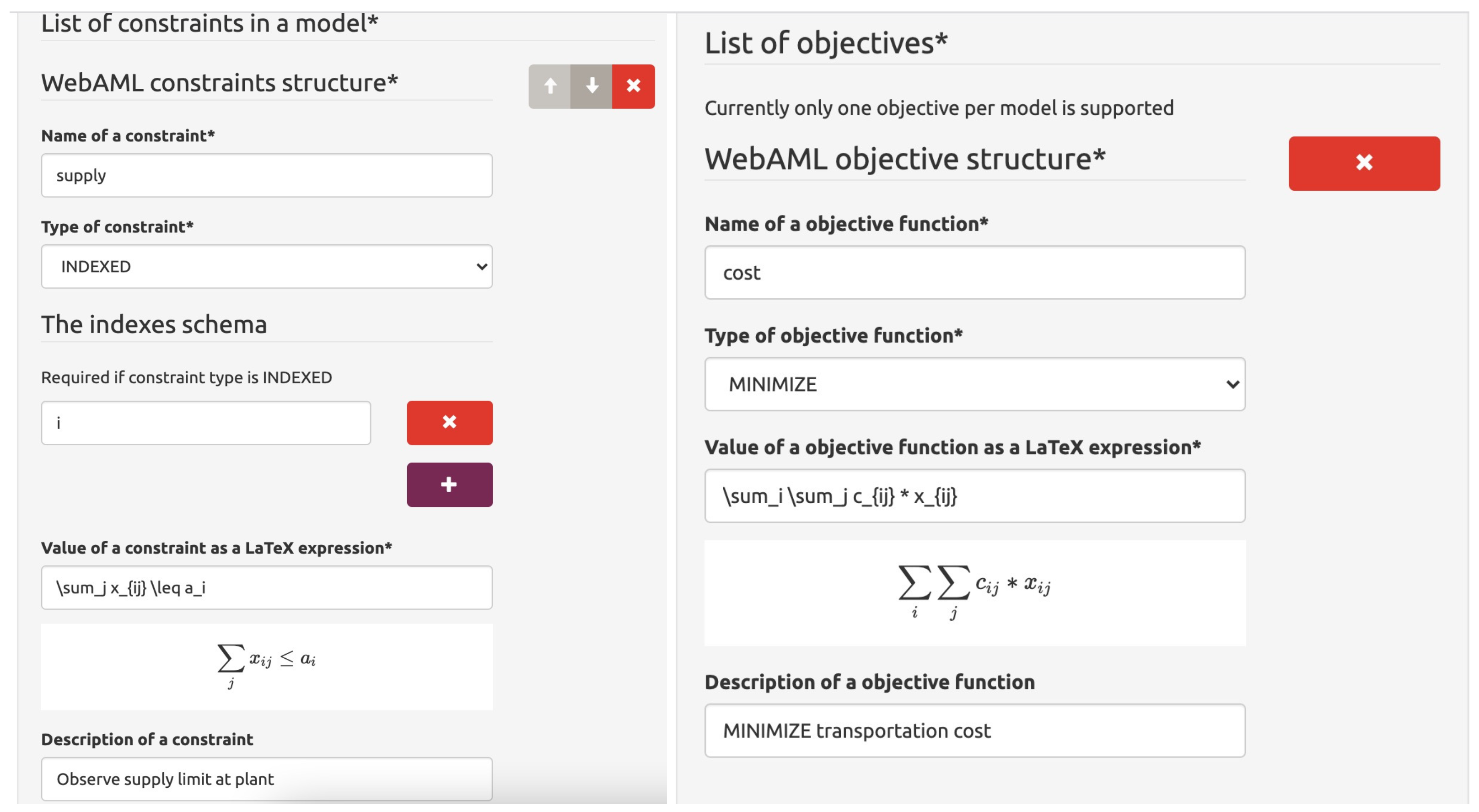
An alternative to capturing optimization problems in a textual format is using a guided user interface proposed in our WebAML Optimization System prototype. In Figure 3, we display how the supply constraint and objective function of a given transportation model instance are captured using the user interface. The user is asked the basic information, such as the type of constraint, indices used in the constraints, and the mathematical expression of the constraint itself.

The constraints are entered using the LATEX mathematical syntax displayed in a visual form to help the user and ensure that valid syntax is used. The objective function is entered similarly. In essence, each type of the model component (set, parameter, constraint, etc.) has its visual representation so that the user experience can be custom tailored to specific kinds of model components. An example of how the solution to the problem and solver output is displayed can be seen in Figure 4.

4.2. Extensibility

We can extend the user interface provided in our prototype further, thus making the process even smoother by giving guiding text and introducing questionnaire-like behavior and similar user experience improvements. We also believe that the architectural decisions made in the design of the WebAML Optimization System make it the foundation for a universal mathematical optimization toolkit. The toolkit could be extended with other state-of-the-art features, such as presolving, distributed solving, or best solver selection based on the model type.

Firstly, one can easily extend WebAML language based on the JSON Schema by introducing new types for the already defined essential components. Listing 7 shows how one could add a new data type called boolean to the set component.

Listing 7. WebAML JSON Schema extended with a new data type for the set component.

"sets": { …      "items": {           …           "properties": {                …                 "valueType": {                      "type": "string",                      "title": "Data type of values in a set",                      "enum": ["STRING", "NUMBER", "BOOLEAN"] // New boolean type                },                …           }      } }

Secondly, one can easily extend the back-end service to support new AMLs by writing a converter from WebAML, thus implementing the WebAMLConverter interface and implementing the AmlFacade interface for integration with the underlying AML binaries. It does not require any changes to be completed in the controller or user interface. Everything is registered automatically and works out of the box after fully implementing the AmlFacade interface provided in Listing 8. There is even an option not to write a special WebAML converter, but to use the GAMS Convert tool as demonstrated in the AmplConverter class.

Listing 8. Structure of AmlFacade interface.

public interface AmlFacade {      boolean isAmlAvailable();      String getAmlName();      List<String> getAvailableSolvers();      AmlResult solveModel(String model, String solver);      String convertModel(String model, String targetAml); }

Finally, one can quickly introduce new features such as presolving or parallel solving by extending the existing ModelController class and adding additional features as an intermediate step between the convert and solve operations.

5. Conclusions and Future Work

In this research, we have identified the major differences and shortcomings amongst four prominent algebraic modeling languages. One is the major is a lack of cross-compatibility, resulting in the difficulty to switch between AMLs and the need to learn the specific syntax. We identify that it can become a challenge in teaching mathematical optimization in schools and universities. To address this and other identified shortcomings, we proposed a new formalized algebraic modeling language (WebAML). We provided the graphical user interface-based open-source tool (WebAML Optimization System) prototype for algebraic modeling and mathematical optimization.

The tool does not require any specific algebraic language knowledge and allows for solving problems using different mathematical optimization solvers. Thus, it simplifies the process of algebraic modeling and mathematical optimization, making it available for individuals without detailed technical knowledge. This makes it appealing not only for enterprise users but also for teachers, lecturers, and students trying to understand the basics of mathematical optimization. Worldwide research of the usage of information and communication technology (ICT) to support, enhance, and optimize information delivery has shown that ICT can lead to improved student learning and better teaching methods (e.g., [43,44,45,46]). The tool also supports all of the solvers available in the underlying AMLs, thus providing a wide range of free and commercial solvers. Since the tool can easily be installed on a server and accessed via a web interface, an institution can acquire a full academic or commercial license and allow easy access for every member to solve large-scale optimization problems.

One possible future research direction could be extending the proposed WebAML language to simplify the model definition process. Improving the user interface (e.g., adding textual guidance) and simplifying the syntax of the language (e.g., support for implicit definition of sets) are among the potential nearest future works. Another research avenue could be the development of extensions to the WebAML Optimization System. Our analysis revealed a need for parallel model generation and presolving capabilities. We have guided how such extensions can be built into our prototype. Further research could be implementing automated solver algorithm selection in the WebAML Optimization System, which would significantly simplify the work for practitioners. Research in automatic algorithm selection is already ongoing and advanced [47]. Finally, testing in real-life situations and improving the existing prototype are needed to make a tool be adopted in mathematics classrooms and by enterprise users.