The Exact Solutions of Stochastic Fractional-Space Kuramoto-Sivashinsky Equation by Using ($\frac{G^{\prime }}{G}$)-Expansion Method

Abstract

In this paper, we consider the stochastic fractional-space Kuramoto–Sivashinsky equation forced by multiplicative noise. To obtain the exact solutions of the stochastic fractional-space Kuramoto–Sivashinsky equation, we apply the $\frac{G^{\prime }}{G}$-expansion method. Furthermore, we generalize some previous results that did not use this equation with multiplicative noise and fractional space. Additionally, we show the influence of the stochastic term on the exact solutions of the stochastic fractional-space Kuramoto–Sivashinsky equation.

1. Introduction

In recent decades, fractional derivatives have received a lot of attention because they have been effectively used to problems in finance [1,2,3], biology [4], physics [5,6,7,8], thermodynamic [9,10], hydrology [11,12], biochemistry and chemistry [13]. Since fractional-order integrals and derivatives allow for the representation of the memory and heredity properties of various substances, these new fractional-order models are more suited than the previously used integer-order models [14]. This is the most important benefit of fractional-order models in comparison with integer-order models, where such impacts are ignored.

On the other hand, fluctuations or randomness have now been shown to be important in many phenomena. Therefore, random effects have become significant when modeling different physical phenomena that take place in oceanography, physics, biology, meteorology, environmental sciences, and so on. Equations that consider random fluctuations in time are referred to as stochastic differential equations.

Recently, some studies on the approximation solutions of fractional differential equations with stochastic perturbations have been published, such as those of Taheri et al. [15], Zou [16], Mohammed et al. [17,18], Mohammed [19], Kamrani [20], Li and Yang [21] and Liu and Yan [22], while the exact solutions of stochastic fractional differential equations have not been discussed until now.

In this study, we take into account the following stochastic fractional-space Kuramoto–Sivashinsky (S-FS-KS) equation in one dimension with multiplicative noise in the itô sense:

$${\partial }_{t}u+ru{D}_x^{\alpha }u+p{D}_x^{2\alpha }u+q{D}_x^{4\alpha }u=\rho u{\partial }_t\beta ,$$

(1)

where r, p, and q are nonzero real constants, $\alpha$ is the order of the fractional space derivative, $\rho$ is the noise strength, and $\beta (t)$ is the standard Gaussian process and it depends only on t.

The deterministic Kuramoto–Sivashinsky Equation (1) (i.e., $\rho =0$) with $\alpha =1$ has been studied by a number of authors to attain its exact solutions by different methods such as the modified tanh-coth method [23], the tanh method and the extended tanh method [24], homotopy analysis method [25], the $(\frac{G^{\prime }}{G})$-expansion method [26], perturbation method [27], the Weiss–Tabor–Carnevale method [28], Painlevé expansion methods [29], the truncated expansion method [30], the polynomial expansion method [31,32,33,34,35,36,37], among many others; see also the references therein.

The motivation of this article is to find the exact solutions of the S-FS-KS (1) derived from multiplicative noise by employing the $(\frac{G^{\prime }}{G})$-expansion method. The results presented here improve and generalize earlier studies, such as those mentioned in [24]. It is also discussed how multiplicative noise affects these solutions. To the best of our knowledge, this is the first paper to establish the exact solution of the S-FS-KS (1).

In the next section, we define the order $\alpha$ of Jumarie’s derivative and we state some significant properties of the modified Riemann–Liouville derivative. In Section 3, we obtain the wave equation for the S-FS-KS Equation (1), while in Section 4 we have the exact stochastic solutions of the S-FS-KS (1) by applying the $(\frac{G^{\prime }}{G})$-expansion method. In Section 5, we show several graphical representations to demonstrate the effect of stochastic terms on the obtained solutions of the S-FS-KS. Finally, the conclusions of this paper are presented.

2. Modified Riemann–Liouville Derivative and Properties

The order $\alpha$ of Jumarie’s derivative is defined by [38]:

$$D_x^{\alpha }g(x)=\left\{\begin{array}{l}\frac{1}{\Gamma (1-\alpha )}\frac{d}{dx}{\int }_0^x{(x-\zeta )}^{-\alpha }(g(\zeta )-g(0))d\zeta ,0<\alpha <1,\\ [g^{(n)}{(x)]}^{\alpha -n},n\le \alpha \le n+1,n\ge 1,\end{array}\right.$$

where g: $\mathbb{R}\to \mathbb{R}$ is a continuous function but not necessarily first-order differentiable and $\Gamma (.)$ is the Gamma function.

Now, let us state some significant properties of modified Riemann–Liouville derivative as follows:

$$D_x^{\alpha }{x}^{\delta }=\frac{\Gamma (1+\delta )}{\Gamma (1+\delta -\alpha )}{x}^{\delta -\alpha },\delta >0,$$

$$D_x^{\alpha }[ag(x)]=a{D}_x^{\alpha }g(x),$$

$$D_x^{\alpha }[af(x)+bg(x)]=a{D}_x^{\alpha }f(x)+b{D}_x^{\alpha }g(x),$$

and

$$D_x^{\alpha }g(u(x))={\sigma }_x\frac{dg}{du}{D}_x^{\alpha }u,$$

where ${\sigma }_x$ is called the sigma indexes [39,40].

3. Wave Equation for S-FS-KS Equation

To obtain the wave equation for the SKS Equation (1), we apply the next wave transformation

$$u(x,t)=\phi (\eta )e^{(\rho \beta (t)-\frac{1}{2}{\rho }^{2}t)},\eta =\frac{1}{\Gamma (1+\alpha )}{x}^{\alpha }-ct,$$

(2)

where $\phi$ is the deterministic function and c is the wave speed. By differentiating Equation (2) with respect to x and t, we obtain

$$\begin{array}{ccc}\hfill u_t& =& (-c{\phi }^{\prime }+\frac{1}{2}{\rho }^2\phi -\frac{1}{2}{\rho }^2\phi +\rho \phi {\beta }_t)e^{(\rho \beta (t)-\frac{1}{2}{\rho }^{2}t)},\hfill \\ \hfill D_x^{\alpha }u& =& {\sigma }_x{\phi }^{\prime }{e}^{[\rho \beta (t)-{\rho }^{2}t]},D_x^{2\alpha }u={\sigma }_x^2{\phi }^{″}{e}^{[\rho \beta (t)-{\rho }^{2}t]}.\hfill \\ \hfill D_x^{3\alpha }& =& {\sigma }_x^3{e}^{(\rho \beta (t)-\frac{1}{2}{\rho }^{2}t)},D_x^{4\alpha }={\sigma }_x^4{e}^{(\rho \beta (t)-\frac{1}{2}{\rho }^{2}t)},\hfill \end{array}$$

(3)

where $+\frac{1}{2}{\rho }^2\phi$ is the Itô correction term. Now, substituting Equation (3) into Equation (1), we obtain

$$-c{\phi }^{\prime }+\tilde{r}\phi {\phi }^{\prime }{e}^{(\rho \beta (t)-\frac{1}{2}{\rho }^{2}t)}+\tilde{p}{\phi }^{″}+\tilde{q}{\phi }^{⁗}=0,$$

(4)

where we put $\tilde{r}={\sigma }_{x}r$, $\tilde{p}={\sigma }_x^{2}p$ and $\tilde{q}={\sigma }_x^{4}q$. Taking the expectation on both sides and considering that $\phi$ is deterministic function, we have

$$-c{\phi }^{\prime }+\tilde{r}\phi {\phi }^{\prime }{e}^{-\frac{1}{2}{\rho }^{2}t}\mathbb{E}(e^{\rho \beta (t)})+\tilde{p}{\phi }^{″}+\tilde{q}{\phi }^{⁗}=0.$$

(5)

Since $\beta (t)$ is standard Gaussian random variable, then for any real constant $\rho$ we have $\mathbb{E}(e^{\rho \beta (t)})=e^{\frac{{\rho }^2}{2}t}.$ Now, Equation (5) has the form

$$-c{\phi }^{\prime }+\tilde{r}\phi {\phi }^{\prime }+\tilde{p}{\phi }^{″}+\tilde{q}{\phi }^{⁗}=0.$$

(6)

Integrating Equation (6) once in terms of $\eta$ yields

$$\tilde{q}{\phi }^{‴}+\tilde{p}{\phi }^{\prime }+\frac{\tilde{r}}{2}{\phi }^2-c\phi =0,$$

(7)

where we set the constant of integration as equal to zero.

4. The Exact Solutions of the S-FS-KS Equation

Here, we apply the $\frac{G^{\prime }}{G}$-expansion method [41] in order to find the solutions of Equation (7). As a result, we have the exact solutions of the S-FS-KS (1). First, we suppose the solution of the S-FS-KS equation, Equation (7), has the form

$$\phi =\sum _{k=0}^M{b}_k{[\frac{G^{\prime }}{G}]}^k,$$

(8)

where $b_0,b_1,...,b_M$ are uncertain constants that must be calculated later, and G solves

$$G^{″}+\lambda G^{\prime }+\mu G=0,$$

(9)

where $\lambda ,\mu$ are unknown constants. Let us now calculate the parameter M by balancing ${\phi }^2$ with ${\phi }^{‴}$ in Equation (7) as follows

$$2M=M+3;$$

hence

$$M=3.$$

(10)

From (10), we can rewrite Equation (8) as

$$\phi =b_0+b_1[\frac{G^{\prime }}{G}]+b_2{[\frac{G^{\prime }}{G}]}^2+b_3{[\frac{G^{\prime }}{G}]}^3.$$

(11)

Putting Equation (11) into Equation (7) and utilizing Equation (9), we obtain a polynomial with degree 6 of $\frac{G^{\prime }}{G}$ as follows

$$\begin{array}{ccc}& & (\frac{1}{2}\tilde{r}{b}_3^2-60\tilde{q}{b}_3){[\frac{G^{\prime }}{G}]}^6+(-24\tilde{q}{b}_2+\tilde{r}{b}_2{b}_3-144\tilde{q}\lambda b_3){[\frac{G^{\prime }}{G}]}^5\hfill \\ & & +(\frac{1}{2}\tilde{r}{b}_2^2-3\tilde{p}{b}_3-6\tilde{q}{b}_1+\tilde{r}{b}_1{b}_3-111\tilde{q}{\lambda }^2{b}_3-114\tilde{q}\mu b_3-54\tilde{q}\lambda b_2){[\frac{G^{\prime }}{G}]}^4\hfill \\ & & +(-c{b}_3+2\tilde{p}{b}_2+\tilde{r}{b}_0{b}_3+\tilde{r}{b}_1{b}_2-3\tilde{p}\lambda b_3-38\tilde{q}{\lambda }^2{b}_2-40\tilde{q}\mu b_2-27{\lambda }^3{b}_3\hfill \\ & & -12\tilde{q}\lambda b_1-168\tilde{q}\lambda \mu b_3){[\frac{G^{\prime }}{G}]}^3+(-c{b}_2+\frac{1}{2}\tilde{r}{b}_1^2-\tilde{p}{b}_1+\tilde{r}{b}_0{b}_2-2\tilde{p}\lambda b_2\hfill \\ & & -3\tilde{p}\mu b_3-7\tilde{q}{\lambda }^2{b}_1-8\tilde{q}\mu b_1-8\tilde{q}{\lambda }^3{b}_2-52\tilde{q}\lambda \mu b_2-60\tilde{q}{\mu }^2{b}_3\hfill \\ & & -57\tilde{q}{\lambda }^2\mu b_3){[\frac{G^{\prime }}{G}]}^2+(-c{b}_1+\tilde{r}{b}_0{b}_1-\tilde{p}\lambda b_1-2\tilde{p}\mu b_2-\tilde{q}{\lambda }^3{b}_1\hfill \\ & & -16\tilde{q}{\mu }^2{b}_2-8\tilde{q}\lambda \mu b_1-14\tilde{q}{\lambda }^2\mu b_2-36\tilde{q}{\mu }^2\lambda b_3)[\frac{G^{\prime }}{G}]+\hfill \end{array}$$

$$(-c{b}_0+\frac{1}{2}\tilde{r}{b}_0^2-\tilde{p}\mu b_1-\tilde{q}{\lambda }^2\mu b_1-6\tilde{q}{\mu }^2\lambda b_2-2\tilde{q}{\mu }^2{b}_1-6\tilde{q}{\mu }^3{b}_3)=0.$$

By equating each coefficient of ${[\frac{G^{\prime }}{G}]}^i$ ($i=6,5,4,3,2,1,0$) to zero, we have a system of algebraic equations. By solving this system by using Maple, we obtain two cases:

First case:

$$\begin{array}{ccc}\hfill b_0& =& \pm \frac{30\tilde{p}}{19\tilde{r}}\sqrt{\frac{-\tilde{p}}{19\tilde{q}}},b_1=\frac{90\tilde{p}}{19\tilde{r}},b_2=0,b_3=\frac{120\tilde{q}}{\tilde{r}},\hfill \\ \hfill c& =& \pm \frac{30\tilde{p}}{19}\sqrt{\frac{-\tilde{p}}{19\tilde{q}}},\lambda =0,\mu =\frac{\tilde{p}}{76\tilde{q}},\mathrm{if}\frac{\tilde{p}}{\tilde{q}}<0.\hfill \end{array}$$

(12)

In this situation, the solution of Equation (7) is

$$\phi (\eta )=b_0+b_1[\frac{G^{\prime }}{G}]+b_3{[\frac{G^{\prime }}{G}]}^3.$$

(13)

By solving Equation (9) with $\lambda =0,\mu =\frac{\tilde{p}}{76\tilde{q}}$ if $\frac{\tilde{p}}{\tilde{q}}<0,$ we obtain

$$G(\eta )=c_{1}exp(\sqrt{\frac{-\tilde{p}}{76\tilde{q}}}\eta )+c_{2}exp(-\sqrt{\frac{-\tilde{p}}{76\tilde{q}}}\eta ),$$

(14)

where $c_1$ and $c_2$ are constants. Putting Equation (14) into Equation (13), we have

$$\begin{array}{ccc}\hfill \phi (\eta )& =& \pm \frac{30\tilde{p}}{19\tilde{r}}\sqrt{\frac{-\tilde{p}}{19\tilde{q}}}+\frac{90\tilde{p}}{19\tilde{r}}\sqrt{\frac{-\tilde{p}}{76\tilde{q}}}[\frac{c_{1}exp(\sqrt{\frac{-\tilde{p}}{76\tilde{q}}}\eta )-c_{2}exp(-\sqrt{\frac{-\tilde{p}}{76\tilde{q}}}\eta )}{c_{1}exp(\sqrt{\frac{-\tilde{p}}{76\tilde{q}}}\eta )+c_{2}exp(-\sqrt{\frac{-\tilde{p}}{76\tilde{q}}}\eta )}]\hfill \\ & & +\frac{120\tilde{q}}{\tilde{r}}{(\sqrt{\frac{-\tilde{p}}{76\tilde{q}}})}^3{[\frac{c_{1}exp(\sqrt{\frac{-\tilde{p}}{76\tilde{q}}}\eta )-c_{2}exp(-\sqrt{\frac{-\tilde{p}}{76\tilde{q}}}\eta )}{c_{1}exp(\sqrt{\frac{-\tilde{p}}{76\tilde{q}}}\eta )+c_{2}exp(-\sqrt{\frac{-\tilde{p}}{76\tilde{q}}}\eta )}]}^3.\hfill \end{array}$$

Hence, the exact solution in this case of the S-FS-KS (1), by using (2), has the form

$$\begin{array}{ccc}\hfill u_1(x,t)& =& e^{(\rho \beta (t)-\frac{1}{2}{\rho }^{2}t)}\{\pm \frac{30\tilde{p}\hslash }{19\tilde{r}}\hfill \\ & & +\frac{90\tilde{p}\hslash }{19\tilde{r}}[\frac{c_{1}exp(\hslash (\frac{1}{\Gamma (1+\alpha )}{x}^{\alpha }-ct))-c_{2}exp(-\hslash (\frac{1}{\Gamma (1+\alpha )}{x}^{\alpha }-ct))}{c_{1}exp(\hslash (\frac{1}{\Gamma (1+\alpha )}{x}^{\alpha }-ct))+c_{2}exp(-\hslash (\frac{1}{\Gamma (1+\alpha )}{x}^{\alpha }-ct))}]\hfill \\ & & +\frac{120\tilde{q}{\hslash }^3}{\tilde{r}}{[\frac{c_{1}exp(\frac{\hslash }{\Gamma (1+\alpha )}{x}^{\alpha }-c\hslash t)-c_{2}exp(-\hslash (\frac{1}{\Gamma (1+\alpha )}{x}^{\alpha }-ct))}{c_{1}exp(\frac{\hslash }{\Gamma (1+\alpha )}{x}^{\alpha }-c\hslash t)+c_{2}exp(-\hslash (\frac{1}{\Gamma (1+\alpha )}{x}^{\alpha }-ct))}]}^3\},\hfill \end{array}$$

(15)

where $c=\pm \frac{30\tilde{p}}{19}\sqrt{\frac{-\tilde{p}}{19\tilde{q}}}$, $\hslash =\sqrt{\frac{-\tilde{p}}{76\tilde{q}}}$ and $\frac{\tilde{p}}{\tilde{q}}<0.$

Second case:

$$\begin{array}{ccc}\hfill b_0& =& \pm \frac{30\tilde{p}}{19\tilde{r}}\sqrt{\frac{11}{19\tilde{q}}},b_1=\frac{-270\tilde{p}}{19\tilde{r}},b_2=0,b_3=\frac{120\tilde{q}}{\tilde{r}},\hfill \\ \hfill c& =& \pm \frac{30\tilde{p}}{19}\sqrt{\frac{11\tilde{p}}{19\tilde{q}}},\lambda =0,\mu =\frac{-11\tilde{p}}{76\tilde{q}},\mathrm{if}\frac{\tilde{p}}{\tilde{q}}>0.\hfill \end{array}$$

(16)

In this situation, the solution of Equation (7) is

$$\phi (\eta )=b_0+b_1[\frac{G^{\prime }}{G}]+b_3{[\frac{G^{\prime }}{G}]}^3.$$

(17)

Solving Equation (9) with $\lambda =0,\mu =\frac{-11p}{76\tilde{q}},$ if $\frac{\tilde{p}}{\tilde{q}}>0,$ we obtain

$$G(\eta )=c_{1}exp(\sqrt{\frac{11\tilde{p}}{76\tilde{q}}}\eta )+c_{2}exp(-\sqrt{\frac{11\tilde{p}}{76\tilde{q}}}\eta ).$$

(18)

Substituting Equation (14) into Equation (13), we have

$$\begin{array}{ccc}\hfill \phi (\eta )& =& \pm \frac{30\tilde{p}}{19\tilde{r}}\sqrt{\frac{11\tilde{p}}{19\tilde{q}}}-\frac{270\tilde{p}}{19\tilde{r}}\sqrt{\frac{11\tilde{p}}{76\tilde{q}}}[\frac{c_{1}exp(\sqrt{\frac{11\tilde{p}}{76\tilde{q}}}\eta )-c_{2}exp(-\sqrt{\frac{11\tilde{p}}{76\tilde{q}}}\eta )}{c_{1}exp(\sqrt{\frac{11\tilde{p}}{76\tilde{q}}}\eta )+c_{2}exp(-\sqrt{\frac{11\tilde{p}}{76\tilde{q}}}\eta )}]\hfill \\ & & +\frac{120\tilde{q}}{\tilde{r}}{(\sqrt{\frac{11\tilde{p}}{76\tilde{q}}})}^3{[\frac{c_{1}exp(\sqrt{\frac{11\tilde{p}}{76\tilde{q}}}\eta )-c_{2}exp(-\sqrt{\frac{11\tilde{p}}{76\tilde{q}}}\eta )}{c_{1}exp(\sqrt{\frac{11\tilde{p}}{76\tilde{q}}}\eta )+c_{2}exp(-\sqrt{\frac{11\tilde{p}}{76\tilde{q}}}\eta )}]}^3.\hfill \end{array}$$

Therefore, by using (2), the exact solution in this case of the S-FS-KS (1) has the form

$$\begin{array}{ccc}\hfill u_2(x,t)& =& e^{(\rho \beta (t)-\frac{1}{2}{\rho }^{2}t)}\{\pm \frac{30\tilde{p}}{19\tilde{r}}\sqrt{\frac{11\tilde{p}}{19\tilde{q}}}\hfill \\ & & -\frac{270\tilde{p}\hslash }{19\tilde{r}}[\frac{c_{1}exp(\hslash (\frac{x^{\alpha }}{\Gamma (1+\alpha )}-ct))-c_{2}exp(-\hslash (\frac{x^{\alpha }}{\Gamma (1+\alpha )}-ct))}{c_{1}exp(\sqrt{\frac{11\tilde{p}}{76\tilde{q}}}(\frac{1}{\Gamma (1+\alpha )}{x}^{\alpha }-ct))+c_{2}exp(-\hslash (\frac{x^{\alpha }}{\Gamma (1+\alpha )}-ct))}]\hfill \\ & & +\frac{120\tilde{q}{\hslash }^3}{\tilde{r}}{[\frac{c_{1}exp(\hslash (\frac{x^{\alpha }}{\Gamma (1+\alpha )}-ct))-c_{2}exp(-\hslash (\frac{x^{\alpha }}{\Gamma (1+\alpha )}-ct))}{c_{1}exp(\hslash (\frac{x^{\alpha }}{\Gamma (1+\alpha )}-ct))+c_{2}exp(-\hslash (\frac{x^{\alpha }}{\Gamma (1+\alpha )}-ct))}]}^3\},\hfill \end{array}$$

(19)

where $c=\pm \frac{30\tilde{p}}{19}\sqrt{\frac{11\tilde{p}}{19\tilde{q}}}$, $\hslash =\sqrt{\frac{11\tilde{p}}{76\tilde{q}}}$ and $\frac{\tilde{p}}{\tilde{q}}>0.$

Special Cases:

Case 1: If we choose $c_1=c_2=1,$ then Equations (15) and (19) become

$$\begin{array}{ccc}\hfill u_1(x,t)& =& e^{(\rho \beta (t)-\frac{1}{2}{\rho }^{2}t)}[\pm \frac{30\tilde{p}}{19\tilde{r}}\sqrt{\frac{-\tilde{p}}{19\tilde{q}}}+\frac{90\tilde{p}\hslash }{19\tilde{r}}tanh(\hslash (\frac{x^{\alpha }}{\Gamma (1+\alpha )}-ct))\hfill \\ & & +\frac{120\tilde{q}{\hslash }^3}{\tilde{r}}{tanh}^3(\hslash (\frac{x^{\alpha }}{\Gamma (1+\alpha )}-ct))],\hfill \end{array}$$

(20)

where $c=\pm \frac{30\tilde{p}}{19}\sqrt{\frac{-\tilde{p}}{19\tilde{q}}}$, $\hslash =\sqrt{\frac{-\tilde{p}}{76\tilde{q}}}$ and $\frac{\tilde{p}}{\tilde{q}}<0,$ and

$$\begin{array}{ccc}\hfill u_2(x,t)& =& e^{(\rho \beta (t)-\frac{1}{2}{\rho }^{2}t)}[\pm \frac{30\tilde{p}}{19\tilde{r}}\sqrt{\frac{11\tilde{p}}{19\tilde{q}}}-\frac{270\tilde{p}\hslash }{19\tilde{r}}tanh(\frac{\hslash x^{\alpha }}{\Gamma (1+\alpha )}-c\hslash t)\hfill \\ & & +\frac{120\tilde{q}}{\tilde{r}}{\hslash }^3{tanh}^3(\frac{\hslash x^{\alpha }}{\Gamma (1+\alpha )}-c\hslash t)],\hfill \end{array}$$

(21)

where $c=\pm \frac{30\tilde{p}}{19}\sqrt{\frac{11\tilde{p}}{19\tilde{q}}}$, $\hslash =\sqrt{\frac{11\tilde{p}}{76\tilde{q}}}$ and $\frac{\tilde{p}}{\tilde{q}}>0.$

Case 2: If we choose $c_1=1$ and $c_2=-1,$ then Equations (15) and (19) become

$$\begin{array}{ccc}\hfill u_1(x,t)& =& e^{(\rho \beta (t)-\frac{1}{2}{\rho }^{2}t)}\{\pm \frac{30p}{19\tilde{r}}\sqrt{\frac{-\tilde{p}}{19\tilde{q}}}+\frac{90\tilde{p}\hslash }{19\tilde{r}}coth(\frac{\hslash x^{\alpha }}{\Gamma (1+\alpha )}-c\hslash t)\hfill \\ & & +\frac{120\tilde{q}{\hslash }^3}{\tilde{r}}{coth}^3(\frac{\hslash x^{\alpha }}{\Gamma (1+\alpha )}-c\hslash t))\},\hfill \end{array}$$

(22)

where $c=\pm \frac{30\tilde{p}}{19}\sqrt{\frac{-\tilde{p}}{19\tilde{q}}}$, $\hslash =\sqrt{\frac{-\tilde{p}}{76\tilde{q}}}$ and $\frac{\tilde{p}}{\tilde{q}}<0,$ and

$$\begin{array}{ccc}\hfill u_2(x,t)& =& e^{(\rho \beta (t)-\frac{1}{2}{\rho }^{2}t)}\{\pm \frac{30\tilde{p}}{19\tilde{r}}\hslash -\frac{270\tilde{p}\hslash }{19\tilde{r}}coth(\frac{\hslash x^{\alpha }}{\Gamma (1+\alpha )}-c\hslash t)\hfill \\ & & +\frac{120\tilde{q}{\hslash }^3}{\tilde{r}}{coth}^3(\frac{\hslash x^{\alpha }}{\Gamma (1+\alpha )}-c\hslash t)\},\hfill \end{array}$$

(23)

where $c=\pm \frac{30\tilde{p}}{19}\sqrt{\frac{11\tilde{p}}{19\tilde{q}}}$, $\hslash =\sqrt{\frac{11\tilde{p}}{76\tilde{q}}}$ and $\frac{\tilde{p}}{\tilde{q}}>0.$

Remark 1.

If we put $\rho =0$ (i.e., Equation (1) without noise) and $\alpha =1$ in Equations (20)–(23), then we obtain the same results stated in [24].

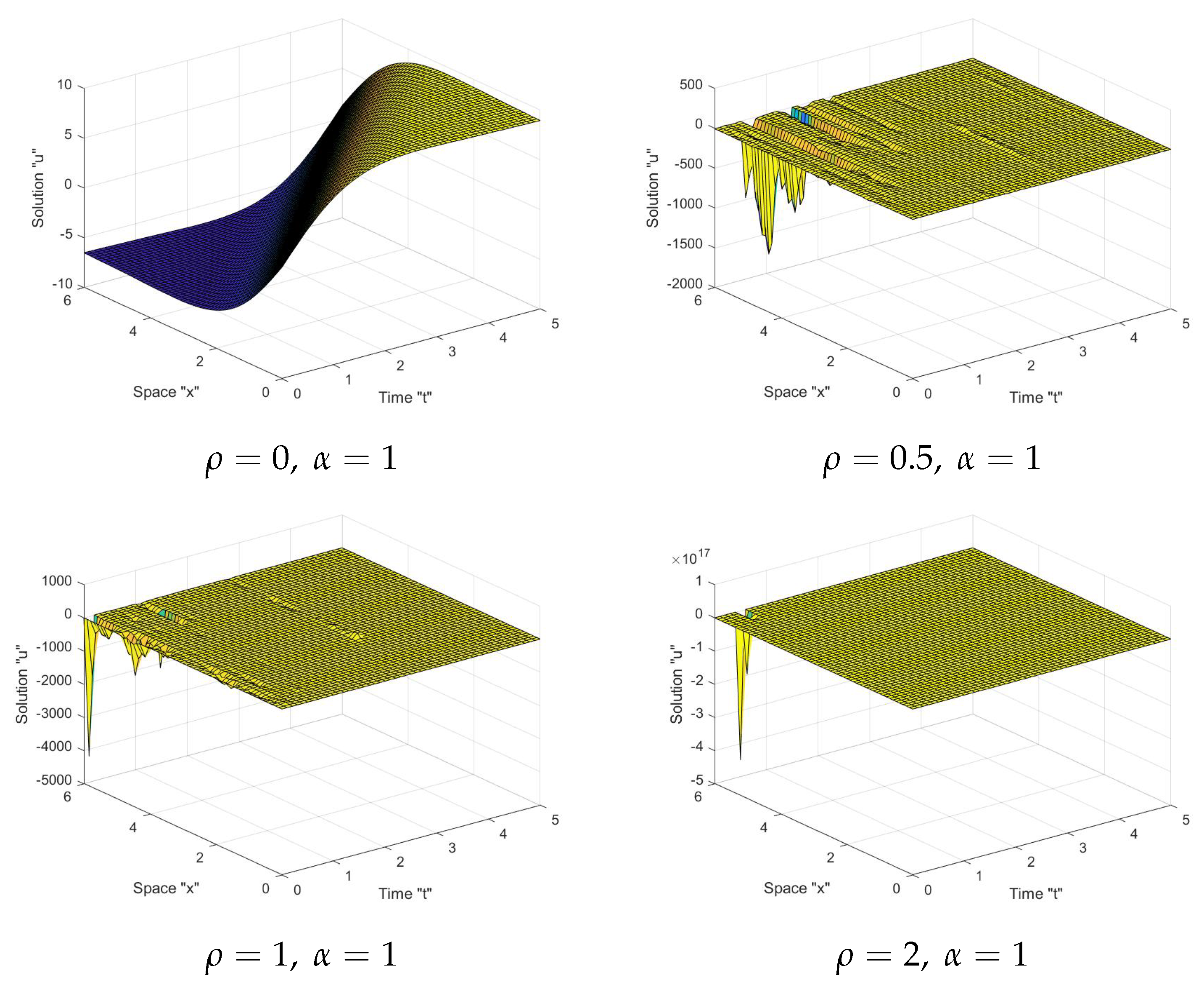
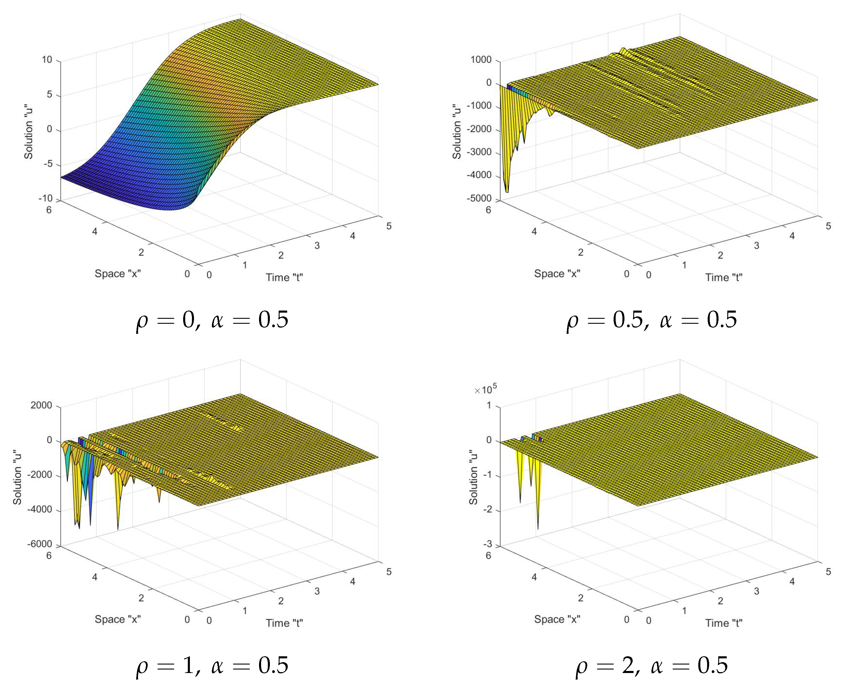
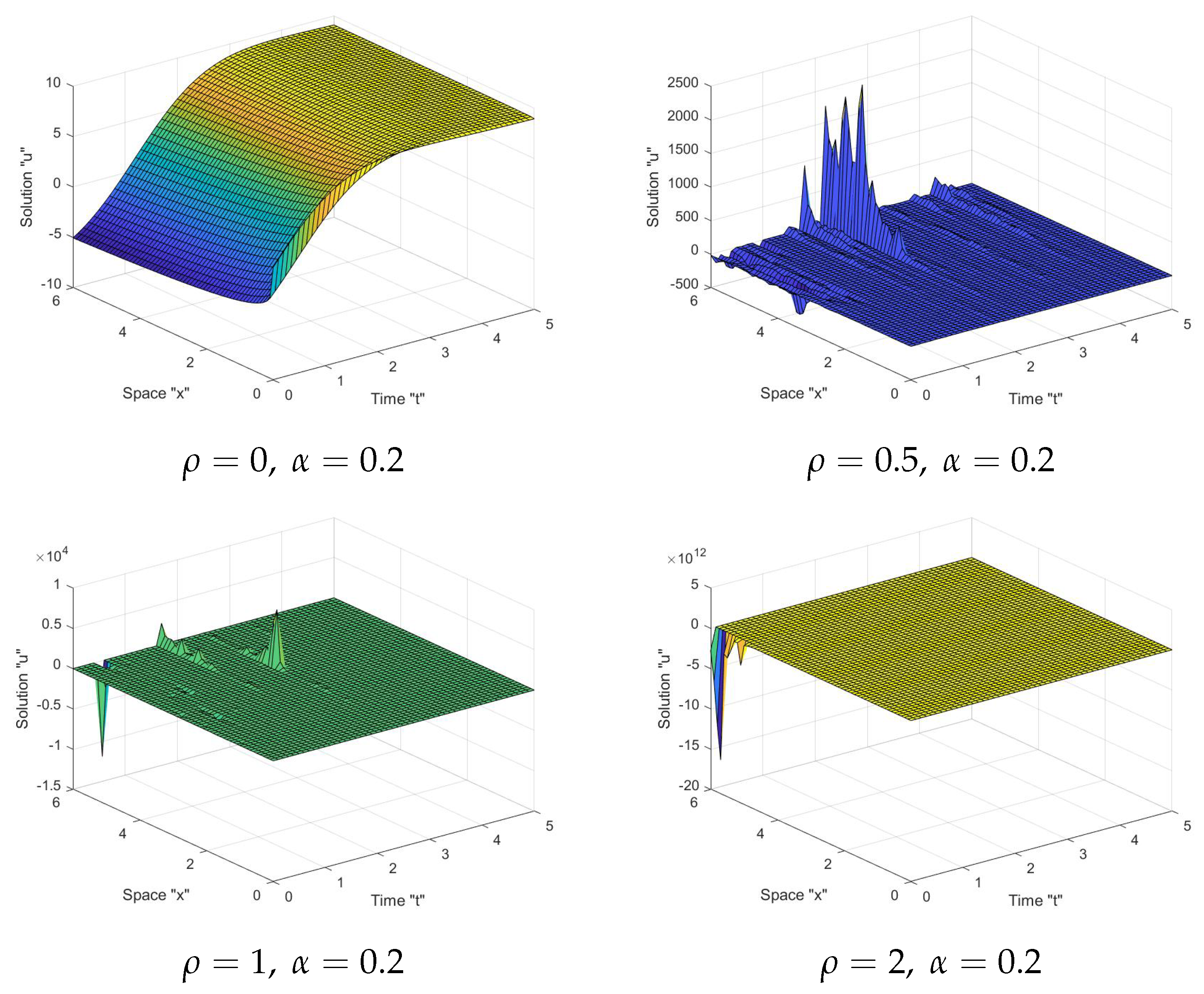
5. The Influence of Noise on the S-FS-KS Solutions

Here, we discuss the influence of stochastic term on the exact solutions of the S-FS-KS Equation (1) and fix the parameters $\tilde{r}=\tilde{p}=\tilde{q}=1$. We present a number of simulations for different values of $\rho$ (noise intensity). We utilize the MATLAB program to plot the solution $u_2(t,x)$ defined in Equation (21) for $t\in [0,5]$ and $x\in [0,6]$ as follows:

In Figure 1, Figure 2 and Figure 3, as seen in the first graph in each figure, the surface becomes less flat when the noise intensity is equal to zero. However, when noise appears and the strength of the noise grows ($\rho =1,2,3$), we notice that the surface becomes more planar after minor transit behaviors. This indicates that the solutions are stable due to the multiplicative noise effects.

6. Conclusions

In this paper, we presented different exact solutions of the stochastic fractional-space Kuramoto–Sivashinsky equation, Equation (1), forced by multiplicative noise. Moreover, several results were extended and improved such as those described in [24]. These types of solutions can be utilized to explain a variety of fascinating and complex physical phenomena. Finally, we used the MATLAB program to generate some graphical representations to show the effect of the stochastic term on the solutions of the S-FS-KS (1). In this paper, we considered the multiplicative noise and fractional space. In future work, we can consider the additive noise and fractional time.

References

1. Gorenflo, R.; Mainardi, F. Random walk models for space—Fractional diffusion processes. Fract. Calc. Appl. Anal. 1998, 1, 167–191. [Google Scholar]
2. Raberto, M.; Scalas, E.; Mainardi, F. Waiting-times and returns in high-frequency financial data: An empirical study. Phys. A Stat. Mech. Appl. 2002, 314, 749–755. [Google Scholar] [CrossRef] [Green Version]
3. Wyss, W. The fractional Black—Scholes equation. Fract. Calc. Appl. Anal. 2000, 3, 51–61. [Google Scholar]
4. Yuste, S.B.; Lindenberg, K. Subdiffusion-limited A+A reactions. Phys. Rev. Lett. 2001, 87, 118301. [Google Scholar] [CrossRef] [Green Version]
5. Barkai, E.; Metzler, R.; Klafter, J. From continuous time random walks to the fractional Fokker—Planck equation. Phys. Rev. E 2000, 61, 132–138. [Google Scholar] [CrossRef]
6. Metzler, R.; Klafter, J. The random walk’s guide to anomalous diffusion: A fractional dynamics approach. Phys. Rep. 2000, 339, 1–77. [Google Scholar] [CrossRef]
7. Saichev, A.I.; Zaslavsky, G.M. Fractional kinetic equations: Solutions and applications. Chaos 1997, 7, 753–764. [Google Scholar] [CrossRef] [PubMed] [Green Version]
8. Zaslavsky, G.M. Chaos, fractional kinetics and anomalous transport. Phys. Rep. 2002, 6, 461–580. [Google Scholar] [CrossRef]
9. Abouelregal, A.E.; Ahmad, H. Thermodynamic modeling of viscoelastic thin rotating microbeam based on non-Fourier heat conduction. Appl. Math. Model. 2021, 91, 973–988. [Google Scholar] [CrossRef]
10. Zenkour, A.M.; Abouelregal, A.E. Effect of harmonically varying heat on FG nanobeams in the context of a nonlocal two-temperature thermoelasticity theory. Eur. J. Comput. Mech. 2014, 23, 1–14. [Google Scholar] [CrossRef]
11. Benson, D.A.; Wheatcraft, S.W.; Meerschaert, M.M. The fractional-order governing equation of Lévy motion. Water Resour. Res. 2000, 36, 1413–1423. [Google Scholar] [CrossRef]
12. Liu, F.; Anh, V.; Turner, I. Numerical solution of the space fractional Fokker—Planck equation. J. Comput. Appl. Math. 2004, 166, 209–219. [Google Scholar] [CrossRef] [Green Version]
13. Yuste, S.B.; Acedo, L.; Lindenberg, K. Reaction front in an A+BC reaction—Subdiffusion process. Phys. Rev. E 2004, 69, 036126. [Google Scholar] [CrossRef] [PubMed] [Green Version]
14. Podlubny, I. Fractional Differential Equations; Academic Press: New York, NY, USA, 1999. [Google Scholar]
15. Taheri, Z.; Javadi, S.; Babolian, E. Numerical solution of stochastic fractional integro-differential equation by the spectral collocation method. J. Comput. Appl. Math. 2017, 321, 336–347. [Google Scholar] [CrossRef]
16. Zou, G. Galerkin finite element method for time-fractional stochastic diffusion equations. Comput. Appl. Math. 2018, 37, 4877–4898. [Google Scholar] [CrossRef]
17. Mohammed, W.W.; Iqbal, N. Effect of the Same Degenerate Additive Noise on a Coupled System of Fractional-Space Diffusion Equations. Fractals. Accepted.
18. Iqbal, N.; Wu, R.; Mohammed, W.W. Pattern formation induced by fractional cross-diffusion in a 3-species food chain model with harvesting. Math. Comput. Simul. 2021, 188, 102–119. [Google Scholar] [CrossRef]
19. Mohammed, W.W. Approximate solutions for stochastic time-fractional reaction—Diffusion equations with multiplicative noise. Math. Methods Appl. Sci. 2021, 44, 2140–2157. [Google Scholar] [CrossRef]
20. Kamrani, M. Numerical solution of stochastic fractional differential equations. Numer. Algorithms 2015, 68, 81–93. [Google Scholar] [CrossRef]
21. Li, X.; Yang, X. Error estimates of finite element methods for stochastic fractional differential equations. J. Comput. Math. 2017, 35, 346–362. [Google Scholar]
22. Liu, J.; Yan, L. Solving a nonlinear fractional stochastic partial differential equation with fractional noise. J. Theor. Probab. 2016, 29, 307–347. [Google Scholar] [CrossRef]
23. Wazzan, L. A modified tanh-coth method for solving the general Burgers-Fisher and Kuramoto-Sivashinsky Equations. Commun. Nonlinear Sci. Numer. Simulat. 2009, 14, 2642–2652. [Google Scholar] [CrossRef]
24. Wazwaz, A.M. New solitary wave solutions to the Kuramoto-Sivashinsky and the Kawahara equations. Appl. Math. Comput. 2006, 182, 1642–1650. [Google Scholar] [CrossRef]
25. Abbasbandy, S. Solitary wave solutions to the Kuramoto—Sivashinsky equation by means of the homotopy analysis method. Nonlinear Dyn. 2008, 52, 35–40. [Google Scholar] [CrossRef]
26. Kheiri, H.; Jabbari, A. Application of the (G′/G)-expansion method for two nonlinear evolution equations. Int. Nonlinear Dyn. Eng. Sci. 2010, 2, 57–67. [Google Scholar]
27. Mohammed, W.W. Approximate solution of the Kuramoto-Shivashinsky equation on an unbounded domain. Chin. Ann. Math. Ser. B 2018, 39, 145–162. [Google Scholar] [CrossRef]
28. Kudryashov, N.A. Exact solutions of the generalized kuramoto-sivashinsky equation. Phys. Lett. A 1990, 147, 287–291. [Google Scholar] [CrossRef]
29. Kudryashov, N.A. On types of nonlinear nonintegrable equations with exact solutions. Phys. Lett. A 1991, 155, 269–275. [Google Scholar] [CrossRef]
30. Kudryashov, N.A.; Soukharev, M.B. Popular ansatz methods and solitary wave solutions of the Kuramoto-Sivashinsky equation. Regul. Chaotic Dyn. 2009, 14, 407–409. [Google Scholar] [CrossRef]
31. Peng, Y.Z. A polynomial expansion method and new general solitary wave solutions to KS equation. Comm. Theor. Phys. 2003, 39, 641–642. [Google Scholar]
32. Kudryashov, N.A. Solitary and periodic solutions of the generalized kuramoto-sivashinsky equation. Regul. Chaotic Dyn. 2008, 13, 234–238. [Google Scholar] [CrossRef]
33. Kudryashov, N.A. Exact soliton solutions of the generalized evolution equation of wave dynamics. J. Appl. Math. Mech. 1988, 52, 361–365. [Google Scholar] [CrossRef]
34. Khalique, C.M. Exact Solutions of the Generalized Kuramoto-Sivashinsky Equation. Casp. J. Math. Sci. 2012, 1, 109–116. [Google Scholar]
35. Zhang, S. New Exact Solutions of the KdV–Burgers–Kuramoto Equation. Phys. Lett. A 2006, 358, 414–420. [Google Scholar] [CrossRef]
36. Blomker, D.; Mohammed, W.W. Amplitude equation for spdes with quadratic nonlinearities. Electron. J. Probab. 2009, 14, 2527–2550. [Google Scholar] [CrossRef]
37. Fu, Z.; Liu, S.; Liu, S. New Exact Solutions to the KdV–Burgers–Kuramoto Equation. Chaos Solitons Fractals 2005, 23, 609–616. [Google Scholar] [CrossRef]
38. Jumarie, G. Modified Riemann–Liouville derivative and fractional Taylor series of nondifferentiable functions further results. Comput. Math. Appl. 2006, 51, 1367–1376. [Google Scholar] [CrossRef] [Green Version]
39. He, J.H.; Elegan, S.K.; Li, Z.B. Geometrical explanation of the fractional complex transform and derivative chain rule for fractional calculus. Phys. Lett. A 2012, 376, 257–259. [Google Scholar] [CrossRef]
40. Aksoy, E.; Kaplan, M.; Bekir, A. Exponential rational function method for space–time fractional differential equations. Waves Random Complex Media 2016, 26, 142–151. [Google Scholar] [CrossRef]
41. Wang, M.L.; Li, X.Z.; Zhang, J.L. The G G -expansion method and travelling wave solutions of nonlinear evolution equations in mathematical physics. Phys. Lett. A 2008, 372, 417–423. [Google Scholar] [CrossRef]
Figure 1. Graph of solution u 2 in Equation (21) with α = 1 .
Mathematics 09 02712 g001
Figure 2. Graph of solution u 2 in Equation (21) with α = 0.5 .
Mathematics 09 02712 g002
Figure 3. Graph of solution u 2 in Equation (21) with α = 0.2 .
Mathematics 09 02712 g003
Publisher’s Note: MDPI stays neutral with regard to jurisdictional claims in published maps and institutional affiliations.