Applying Heath-Jarrow-Morton Model to Forecasting the US Treasury Daily Yield Curve Rates

Abstract

The Heath-Jarrow-Morton (HJM) model is a powerful instrument for describing the stochastic evolution of interest rate curves under no-arbitrage assumption. An important feature of the HJM approach is the fact that the drifts can be expressed as functions of respective volatilities and the underlying correlation structure. Aimed at researchers and practitioners, the purpose of this article is to present a self-contained, but concise review of the abstract HJM framework founded upon the theory of interest and stochastic partial differential equations in infinite dimensions. To illustrate the predictive power of this theory, we apply it to modeling and forecasting the US Treasury daily yield curve rates. We fit a non-parametric model to real data available from the US Department of the Treasury and illustrate its statistical performance in forecasting future yield curve rates.

1. Introduction

Stocks and bonds play a crucial role in making investment decisions. However, there is a significant difference between stock and bond markets. A stock market is a platform enabling companies to issue their shares and trade them on a stock exchange. Buying these shares and having ownership stake, investors can benefit from the performance of the issuer in the future. In contrast, a bond market is used for issuing and trading debt securities. Usually, an investor and a bond issuer make a contract enabling the former to benefit from the interest paid on a regular basis and full nominal amount received when reaching maturity. The bond issuer may be a government, a corporation, etc.

Besides, there are bonds that do not pay an intermediate interest but are traded at a deep discount, rendering profit at the maturity when they are redeemed for their full face value. These bonds are called zero-coupon bonds. For a maturity $T\ge 0$, let $P(t,T)$ denote the price of a zero-coupon bond at time $t\in [0,T]$. It is known from the theory of interest rates (viz. Definition 10 in Section 2) that the instantaneous forward rate of a zero-coupon bond is given by

$$f(t,T)=-\frac{\partial \ln P(t,T)}{\partial T} \mathrm{for} \mathrm{all} t\in [0,T], T>0.$$

(1)

Under appropriate assumptions, Heath, Jarrow and Morton [1] demonstrated that $f(t,T)$ can be modeled as a Markovian diffusion that evolves according to the following stochastic differential equation (SDE):

$$\left\{\begin{array}{ccc}\hfill \mathrm{d}f(t,T)& =& \alpha (t,T)\mathrm{d}t+\sigma (t,T)·\mathrm{d}W\left(t\right),\hfill \\ \hfill f(0,T)& =& f^0\left(T\right),\hfill \end{array}\right.$$

(2)

where ${\left(W\left(t\right)\right)}_{t\in [0,T]}$ is a d-dimensional standard Brownian motion, $T\mapsto f^0\left(T\right)$ is the market instantaneous forward curve at time $t=0$, ${\left(\alpha (t,T)\right)}_{t\in [0,T]}$ and ${\left(\sigma (t,T)\right)}_{t\in [0,T]}$ are 1- and d-dimensional stochastic processes adapted to the natural filtration of ${\left(W\left(t\right)\right)}_{t\in [0,T]}$ and $\sigma (t,T)·\mathrm{d}W\left(t\right)={\sum }_{k=1}^d{\sigma }_k(t,T)\mathrm{d}{W}_k\left(t\right)$ is formally defined as the scalar product. Under suitable regularity assumptions, integrating Equation (2) over $[0,t]$ for $t\in [0,T]$, the instantaneous forward rate $f(t,T)$ can be represented as an Itô-process:

$$f(t,T)=f(0,T)+{\int }_0^t\alpha (s,T)\mathrm{d}s+{\int }_0^t\sigma (s,T)·\mathrm{d}W\left(s\right).$$

(3)

However, the dynamics in Equation (2) is not necessarily arbitrage-free. In the spirit of [2], we understand the presence of arbitrage as the existence of a self-financing strategy which yields a positive income in the future without investing a positive amount today (cf. Section 4). It was further proved in [3] that the existence of an equivalent martingale measure implies the absence of arbitrage opportunities. It was also shown that the unique equivalent martingale measure exists if the drift $\alpha$ depends on the volatility $\sigma$ (see ([2], Chapter 2) for details). In particular, the requirement that the evolution in Equation (2) is taking place under a risk-neutral measure $\mathbb{Q}$ necessitates the following representation:

$$\alpha (t,T)=\sigma (t,T)·{\int }_t^T\sigma (t,s)\mathrm{d}s={\displaystyle \sum }_{k=1}^d{\sigma }_k(t,T){\int }_t^T{\sigma }_k(t,s)\mathrm{d}s \mathrm{for} \mathrm{all} t\in [0,T].$$

Therefore, for all $t\in [0,T]$, we conclude that $f(t,T)$ is fully specified (as a stochastic process) as long as the volatility vector $\sigma$ is provided:

$$f(t,T)=f(0,T)+{\displaystyle \sum }_{k=1}^d{\int }_0^t{\sigma }_k(\tau ,T){\int }_{\tau }^T{\sigma }_k(\tau ,s)\mathrm{d}s\mathrm{d}\tau +{\displaystyle \sum }_{k=1}^d{\int }_0^t{\sigma }_k(s,T)\mathrm{d}{W}_k\left(s\right).$$

Recalling Equation (1), Itô’s lemma furnishes the following SDE for the zero-coupon bond price $P(t,T)$ for all $t\in [0,T]$:

$$\mathrm{d}P(t,T)=P(t,T)\left(r_t \mathrm{d}t-\left({\int }_t^T\sigma (t,s)\mathrm{d}s\right)\mathrm{d}W\left(t\right)\right),$$

where $r_t$ is the instantaneous short-term interest rate at t given by

$$\begin{array}{cc}\hfill r_t& =f(t,t)=f(0,t)+{\int }_0^t\sigma (\tau ,t){\int }_{\tau }^t\sigma (\tau ,s)\mathrm{d}s\mathrm{d}\tau +{\int }_0^t\sigma (s,t)\mathrm{d}W\left(s\right)\hfill \\ \hfill & =f(0,t)+{\displaystyle \sum }_{k=1}^d{\int }_0^t{\sigma }_k(\tau ,t){\int }_{\tau }^t{\sigma }_k(\tau ,s)\mathrm{d}s\mathrm{d}\tau +{\displaystyle \sum }_{k=1}^d{\int }_0^t{\sigma }_k(s,t)\mathrm{d}{W}_k\left(s\right).\hfill \end{array}$$

In his dissertation [4], Filipović proposed to extend this approach to an infinite-dimensional framework and consider the following stochastic partial differential equation (SPDE):

$$\left\{\begin{array}{ccc}\hfill \mathrm{d}{f}_t\left(x\right)& =& (\frac{\mathrm{d}}{\mathrm{d}x}{f}_t\left(x\right)+{\alpha }_t\left(x\right))\mathrm{d}t+{\sigma }_t\left(x\right)·\mathrm{d}W\left(t\right),\hfill \\ \hfill f_t\left(x\right)& =& f^0\left(x\right),\hfill \end{array}\right.$$

(4)

with the so-called Musiela’s notation (cf. [5]) $f_t\left(x\right):=f(t,t+x)$, $x\in [0,T-t]$ being employed (see also [6], Chapter 6). Here, ${\left(W\left(t\right)\right)}_{t\in [0,T]}$ is an infinite-dimensional vector of (coutably many) independent real-valued Brownian motions, the forward rate curve $x\mapsto f_t\left(x\right)$ is a random variable taking its values in a function space $\mathcal{H}$ and the drift $\alpha$ is given by the no-arbitrage condition

$$\begin{array}{c}\hfill {\alpha }_t\left(x\right):=\alpha (t,t+x)={\displaystyle \sum }_{k=1}^{\infty }{\sigma }_k(t,t+x)\left({\int }_0^x{\sigma }_k(t,t+s)\mathrm{d}s\right).\end{array}$$

To facilitate the analytic treatment of Equation (4), we put it into the framework of abstract operator SDEs with stochastic coefficients:

$$\left\{\begin{array}{ccc}\hfill \mathrm{d}{X}_t& =& (A{X}_t+F(t,X_t))\mathrm{d}t+B(t,X_t)\mathrm{d}W\left(t\right),\hfill \\ \hfill X_0& =& X^0,\hfill \end{array}\right.$$

(5)

where X is an $\mathcal{H}$-valued random process, $X^0$ is a random $\mathcal{H}$-valued ${\mathcal{F}}_0$-measurable initial value, $A:\mathcal{H}\to \mathcal{H}$ is a linear (possibly unbounded) operator, ${\left(W\left(t\right)\right)}_{t\in [0,T]}$ is a standard cylindrical Wiener process over $\mathcal{U}$, $F:[0,T]\times \mathsf{\Omega }\times \mathcal{H}\to \mathcal{H}$, $B:[0,T]\times \mathsf{\Omega }\times \mathcal{H}\to {\mathcal{L}}_{\mathrm{HS}}(\mathcal{U},\mathcal{H})$ and $\mathcal{H}$, $\mathcal{U}$ are separable Hilbert spaces. Here and in the sequel, ${\mathcal{L}}_{\mathrm{HS}}(·,·)$ denotes the space of Hilbert-Schmidt operators (cf. Definition A8). Letting

$$\begin{array}{c}\hfill A:=\frac{\mathrm{d}}{\mathrm{d}x}, X_t:=f_t, F:={\alpha }_t, B:=⟨{\sigma }_t,·⟩.\end{array}$$

we can easily see that Equation (4) is a special case of Equation (5). A straightforward integration of Equation (5) over $[0,t]$ yields the integral formulation of Equation (5):

$$X_t=X^0+{\int }_0^t\left(A{X}_s+F(s,X_s)\right)\mathrm{d}s+{\int }_0^{t}B(s,X_s)\mathrm{d}W\left(s\right) \mathrm{for} \mathrm{all} t\in [0,T].$$

(6)

The rest of the paper is structured as follows. Section 2, Section 3 and Section 4 are meant to provide a concise review of the HJM framework and related results. With most of the results being scattered over a number of articles and monographs, our thrust was to give a coherent presentation on this matter with consistent terminology and notation to make the theory better accessible to a broad scientific and professional audience. In Section 2, a brief summary of the interest rate theory is given, in particular, a relation between the price of a zero-coupon bond and its instantaneous forward rate from Equation (1) is established. In Section 3, we introduce the abstract HJM model first presented and studied by [4,6], discuss major advantages of this approach and protocol some known well-posedness results. In Section 4, we summarize central properties of the abstract HJM model, in particular, we give sufficient conditions under which the abstract HJM model defines an arbitrage-free market, describe the long rates associated with the model, and give an example of a state space compatible with the instantaneous forward rate dynamics. Section 5 contains the main contribution of this paper. A (semi-)implicit numerical scheme is developed and applied to Equation (4). Using real data from the US Department of the Treasury [7], the resulting non-parametric model is calibrated using a custom-developed least-squares-like procedure involving principal component analysis (PCA) for parameter estimation and dimension reduction. The simplicity of our approach is one of its main advantages. Indeed, it does not rely on any sophisticated optimization techniques or third-party libraries, thus, making itself attractive and accessible to a wide audience. The model is then deployed to forecast future yield curve rates, estimate the mean future yield curve and compute prediction regions. Using the predictive power of the model as a benchmark measure in lieu of the mere calibration quality is another novelty of our contribution. To the best of our knowledge, this is the first time an infinite-dimensional model is applied to analyze the US Treasury’s daily yield curve rates. We refer [8,9,10] for the finite-dimensional treatise. In Section 6, conclusions are presented. Appendix A, Appendix B and Appendix C contain all seminal probabilistic and functional-analytic concepts and results [6,11,12,13,14,15] used in the article.

2. Interest Rate Theory

Before presenting the abstract Heath-Jarrow-Morton model in Section 3, we give a concise summary of the theory of interest rates based on ([2] pp. 2–18). The goal of this section is twofold. First, we want to give motivation for using the theory of interest rates in this paper. Second, we aim to prove relation (1) between the price and the instantaneous forward rate of a zero-coupon bond in order to define the abstract HJM model afterwards.

As pointed out in ([16], Chapter 25), multivariate (or multidimensional) models have numerous advantages over single-state short rate models, in particular, in describing the intrinsic volatility structure or explaining the inversion of the yield curve, etc. The HJM framework, being at “the far end of this [multivariate] spectrum” (cf. [16], p. 388), is, probably, the most comprehensive one as it employs the forward rate curve as an infinite-dimensional state variable. We refer to the aforecited monograph as well as ([17], pp. 242–245) for further discussions.

Application areas of the HJM framework are very diverse. They include, but are not limited to, modeling of interest futures [18], risk management [19], American option pricing [20], credit risk modeling [21], investment management [22], etc.

2.1. Bank Account and Short Rate

Depositing a certain amount of money in a bank account is typically expected to guarantee its growth at some rate. We need appropriate definitions to express this concept in mathematical terms. Consider a bank account which represents a riskless investment with the profit accruing continuosly.

Definition 1

(Bank account). Let $B\left(t\right)$ be the value of a bank account at time $t\ge 0$. We assume that the bank account evolves according to the differential equation

$$\left\{\begin{array}{ccc}\hfill \mathrm{d}B\left(t\right)& =& r_{t}B\left(t\right)\mathrm{d}t,\hfill \\ \hfill B\left(0\right)& =& B_0,\hfill \end{array}\right.$$

(7)

where $r_t$ is a positive function of time. Letting $B_0=1$, we have

$$B\left(t\right)=\exp \left({\int }_0^t{r}_s\mathrm{d}s\right).$$

(8)

Definition 1 suggests that a unit amount invested at $t=0$ has value (8) at $t>0$, implying also that $B\left(t\right)$ accrues at the short rate $r_t$.

In fact, the first-order Taylor expansion of $B(t+\Delta t)$ is

$$\begin{array}{c}\hfill B(t+\Delta t)=B\left(t\right)(1+r_t\Delta t),\end{array}$$

whence

$$\begin{array}{c}\hfill \frac{B(t+\Delta t)-B\left(t\right)}{B\left(t\right)}=r_t\Delta t \mathrm{as} \Delta t\to 0.\end{array}$$

Definition 2

(Numéraire). A numeraire is any positive non-dividend-paying asset.

Remark 1.

The concept of bank account numéraire is important for relating amounts of currencies available at different times. Assume for simplicity that $r_t$ is deterministic. If K units of currency are deposited into a bank account at the time $t=0$, the amount of units of currency at time $t\ge 0$ is $KB\left(t\right)$. Analogously, the amount is $KB\left(T\right)$ at time $T\ge t$. If we want to have one unit of currency at time T, i.e., $KB\left(T\right)=1$, we have to initially invest $K=1/B\left(T\right)$. Hence, the value of the invested amount K at time t is

$$\begin{array}{c}\hfill KB\left(t\right)=\frac{B\left(t\right)}{B\left(T\right)}.\end{array}$$

Remark 1 motivates the following definition (cf. [2], Chapter 1).

Definition 3

(Stochastic discount factor). The amount at time t “equivalent” to one unit of currency payable at time T

$$\begin{array}{c}\hfill D(t,T)=\frac{B\left(t\right)}{B\left(T\right)}=\exp \left(-{\int }_t^T{r}_s\mathrm{d}s\right).\end{array}$$

is referred to as stochastic discount factor.

2.2. Zero-Coupon Bonds and Spot Interest Rates

Definition 4

(Zero-coupon bond).A zero-coupon bond is a contract that entitles its holder to a (single) payment of one unit of currency at maturity T. Denoting the contract value at time $t\le T$ by $P(t,T)$, we observe $P(T,T)=1$ for all $T\ge 0$.

Definition 5

(Time to maturity). The amount of time $T-t$ from the present moment of time t to the maturity time $T>t$ is referred to as time to maturity $T-t$.

Obviously, $T-t$ is well-defined if t and T are real numbers associated with some time instants. However, if t and T denote two dates $D_1,D_2$, e.g., of format (month/day/year), we can define the amount of time between them in terms of the number of days. Moreover, the number of days between $D_1$ and $D_2$ is calculated according to appropriate market convention, which specifies how these days are to be counted.

Definition 6

(Year fraction). Let $\tau (t,T)$ denote a time measure between t and T, which is usually referred to as year fraction between the dates t and T. If t and T are less than one day apart (typically, occuring when dealing with limiting quantities which involve time to maturities tending to zero), $\tau (t,T)$ is roughly given by $T-t$. A particular choice is known as the day-count convention (see [2,23] for examples).

Additionally, we have to exploit another feature of the zero-coupon bonds called the compounding type in order to switch from the price of a zero-coupon bond and its instantaneous forward rate and vice versa.

Definition 7

(Continuously-compounded spot interest rate). The (constant) rate

$$\begin{array}{c}\hfill R(t,T):=-\frac{\ln P(t,T)}{\tau (t,T)}\end{array}$$

at which an investment of amount $P(t,T)$ at time t accrues continuously to produce a unit amount of currency at maturity T is referred to as continuously-compounded spot interest rate.

Definition 8

(Simply-compounded spot interest rate). Given an initial capital of $P(t,T)$ at time t and assumning accruing takes place proportionally to the investment time, the (constant) rate

$$\begin{array}{c}\hfill L(t,T):=\frac{1-P(t,T)}{\tau (t,T)P(t,T)}\end{array}$$

at which money needs to be invested to yield a single unit of currency at maturity T is called the simply-compounded spot interest.

2.3. Forward Rates

Forward rates are interest rates that can be locked in on a particular day for an investment in a future time period. They are characterized by three time instants: the time t at which the rate is considered, its expiry T and its maturity S, $t<T<S$.

The forward rate can be also viewed as a typical forward rate agreement represented by a contract involving three time characteristics: the current time t, the expiry time $T>t$ and the maturity $S>T$. It enables the investor to benefit from the interest paid between T and S. Moreover, it is possible to fix the interest between T and S at rate K with simply-compounded contract rates, implying a payment of $\tau (T,S)L(T,S)N$ and a receipt of $\tau (T,S)KN$, with N denoting the contract nominal value. This renders the contract value to be $N\tau (T,S)\left(K-L(T,S)\right)$. Recalling Definition 8, the former quantity rewrites it as

$$N\left(\tau (T,S)K-\frac{1}{P(T,S)}+1\right).$$

(9)

Let $1/P(T,S)$ be the amount of currency held at time S. Its value at time T is obtained by multiplying this amount with the zero coupon price $P(T,S)$, i.e.,

$$\begin{array}{c}\hfill P(T,S)\left(1/P(T,S)\right)=1,\end{array}$$

so this term is equivalent to holding one unit of currency at the time T. Besides, one unit of currency at the time T is worth $P(t,T)$ units of currency at the time t. Therefore, the amount $1/P(T,S)$ in S is equivalent to an amount of $P(t,T)$ in t. Now, consider the remaining terms in Equation (9). The worth of $W:=\tau (T,S)K+1$ at the maturity S at the time t is

$$\begin{array}{c}\hfill P(t,S)W=P(t,S)\tau (T,S)K+P(t,S).\end{array}$$

Therefore, the total value of the contract at the time t is

$$N\left(P(t,S)\tau (T,S)K-P(t,T)+P(t,S)\right).$$

(10)

Remark 2.

The value of K rendering the contract in Equation (10) fair at the time t is unique.

Definition 9

(Simply-compounded forward interest rate). Given expiry $T>t$ and maturity $S>T$, the simply-compounded forward interest rate at time t reads as

$$\begin{array}{c}\hfill F(t;T,S):=\frac{1}{\tau (T,S)}\left(\frac{P(t,T)}{P(t,S)}-1\right).\end{array}$$

As the maturity of the forward rate approches its expiry, the concept of instantaneous forward rate emerges. If S is sufficiently close to T, then $\tau (T,S)=S-T$ and we have:

$$\begin{array}{cc}\hfill \underset{S\to T}{\lim }F(t;T,S)& =-\underset{S\to T}{\lim }\frac{1}{P(t,S)}\frac{P(t,S)-P(t,T)}{S-T}\hfill \\ \hfill & =-\frac{1}{P(t,T)}\frac{\partial P(t,T)}{\partial T}\hfill \\ \hfill & =-\frac{\partial \ln P(t,T)}{\partial T}.\hfill \end{array}$$

This motivates the following definition.

Definition 10

(Instantaneous forward interest rate). The instantaneous forward interest rate prevailing at time t for the maturity $T>t$ is denoted by $f(t,T)$ and given as

$$\begin{array}{c}\hfill f(t,T)=\underset{S\to T}{\lim }f(t;T,S)=-\frac{\partial \ln P(t,T)}{\partial T}.\end{array}$$

Remark 3.

Using Musiela’s notation (viz. [5]), $f_t\left(x\right):=f(t,t+x)$ for $x=T-t$ and $t,x\ge 0$. The space of functions $f_t$ will be denoted by $\mathcal{S}$ and called the state space.

3. The Abstract Heath-Jarrow-Morton Model

Filipović [4] proposed to model the instantaneous forward rate of a zero-coupon bond via an infinite-dimensional SDE driven by the standard cylindrical Wiener process. In contrast to the standard finite-dimensional Heath-Jarrow-Morton (HJM) framework, the underlying bond market captures the entire (unobservable) infinite-dimensional interest rate term structure. Among many other advantages, the infinite-dimensional HJM model mitigates the so-called “maturity specific risk” typically present in finite-dimensional models. For a more detailed discussion of infinite-dimensional models, the reader may be referred to the monograph ([6], Chapter 6.5). Also, it gives a natural way to “extrapolate” outside of the original finite maturity grid. From the empirical point of view, the infinite-dimensional structure of the model not only helps better mimic the observed dynamics by merely increasing the “number” of model parameters, but makes it possible to capture the non-trivial topological aspects of the dynamics, thus, improving the predictive power and allowing for natural dimension reduction or regularization without resorting to ad hoc penalties. Arguably, this justifies the increased price associated with the infinite-dimensional functional-analytic and probabilistic framework.

In this section, we introduce the abstract HJM model following the approach of [4,6]. The resulting model is a semilinear stochastic PDE (SPDE) driven by the standard cylindrical Wiener process (see Appendix C). The well-posedness of these abstract SPDEs in the class of mild solutions is obtained using the abstract results from ([11], Chapter 7) and discussed in Section 3.1. The results are then applied to justify the well-posedness of the abstract HJM model to be introduced in Section 3.2.

3.1. Existence and Uniqueness of Mild Solutions to Semilinear Spdes

We consider the abstract SPDE

$$\left\{\begin{array}{ccc}\hfill \mathrm{d}{X}_t& =& \left(A{X}_t+F(t,X_t)\right)\mathrm{d}t+B(t,X_t)\mathrm{d}W\left(t\right),\hfill \\ \hfill X_0& =& X^0\hfill \end{array}\right.$$

(11)

and investigate the existence and uniqueness of mild solutions. Depending on the context, the solution process will be denoted as ${\left(X_t\right)}_{t\in [0,T]}$ or ${\left(X\left(t\right)\right)}_{t\in [0,T]}$. Let $\left(\mathsf{\Omega },\mathcal{F},{\left\{{\mathcal{F}}_t\right\}}_{t\ge 0},\mathbb{P}\right)$ be a filtered probability space and let $T>0$. Let ${\mathcal{P}}_T$ and ${\mathcal{P}}_{\infty }$ denote the predictable $\sigma$-algebras on $[0,T]\times \mathsf{\Omega }$ and $[0,\infty )\times \mathsf{\Omega }$, respectively. We also assume that $\mathcal{U}$, $\mathcal{H}$ are separable Hilbert spaces and ${\left(W\left(t\right)\right)}_{t\in [0,T]}$ is a standard cylindrical Wiener process over $\mathcal{U}$ given in Definition A7. Therefore, using the notation of Appendix C.1, we can let $Q=I$ and ${\mathcal{U}}_0=Q^{\frac{1}{2}}\mathcal{U}\equiv \mathcal{U}$. The spaces $\mathcal{U}$, $\mathcal{H}$, ${\mathcal{L}}_{\mathrm{HS}}(\mathcal{U},\mathcal{H})$ induce corresponding Borel $\sigma$-algebras $\mathcal{B}\left(\mathcal{U}\right)$, $\mathcal{B}\left(\mathcal{H}\right)$, $\mathcal{B}\left({\mathcal{L}}_{\mathrm{HS}}(\mathcal{U},\mathcal{H})\right)$. (Recall that ${\mathcal{L}}_{\mathrm{HS}}(·,·)$ denotes the space of Hilbert-Schmidt operators.) Lastly, $X^0$ is a random $\mathcal{H}$-valued ${\mathcal{F}}_0$-measurable initial value. See Appendix A and Appendix C for a brief review of probabilistic concepts and results used in this section.

Assumption 1.

Let A, F and B in Equation (11) satisfy:

• $F:[0,T]\times \mathsf{\Omega }\times \mathcal{H}\to \mathcal{H}$ is measurable from $\left([0,T]\times \mathsf{\Omega }\times \mathcal{H},{\mathcal{P}}_T\times \mathcal{B}\left(\mathcal{H}\right)\right)$ to $\left(\mathcal{H},\mathcal{B}\left(\mathcal{H}\right)\right)$,
• $B:[0,T]\times \mathsf{\Omega }\times \mathcal{H}\to {\mathcal{L}}_{\mathrm{HS}}(\mathcal{U},\mathcal{H})$ is measurable from $\left([0,T]\times \mathsf{\Omega }\times \mathcal{H},{\mathcal{P}}_T\times \mathcal{B}\left(\mathcal{H}\right)\right)$ to $\left({\mathcal{L}}_{\mathrm{HS}}(\mathcal{U},\mathcal{H}),\mathcal{B}\left({\mathcal{L}}_{\mathrm{HS}}(\mathcal{U},\mathcal{H})\right)\right)$,
• There exists a constant $C>0$ such that for all $u,v\in \mathcal{H}$, $t\in [0,T]$, $\omega \in \mathsf{\Omega }$ we have:

  $$\begin{array}{cc}\hfill {\parallel F(t,\omega ,u)-F(t,\omega ,v)\parallel }_{\mathcal{H}}+{\parallel B(t,\omega ,u)-B(t,\omega ,v)\parallel }_{{\mathcal{L}}_{\mathrm{HS}}(\mathcal{U},\mathcal{H})}& \le C{\parallel u-v\parallel }_{\mathcal{H}},\hfill \\ \hfill {\parallel F(t,\omega ,u)\parallel }_{\mathcal{H}}^2+{\parallel B(t,\omega ,u)\parallel }_{{\mathcal{L}}_{\mathrm{HS}}(\mathcal{U},\mathcal{H})}^2& \le C^2\left(1+{\parallel u\parallel }_{\mathcal{H}}^2\right),\hfill \end{array}$$
• A is the generator of a strongly continuous operator semigroup ${\left(S_t\right)}_{t\ge 0}$ on $\mathcal{H}$.

Definition 11

(Mild Solution). An $\mathcal{H}$-valued predictable stochastic process ${\left(X\left(t\right)\right)}_{t\in [0,T]}$ with

$$\begin{array}{c}\hfill \mathbb{P}\left({\int }_0^T{\parallel X\left(s\right)\parallel }_{\mathcal{H}}^2\mathrm{d}s<\infty \right)=1\end{array}$$

is referred to as a mild solution to Equation (11) if it satisfies the integral equation (well-defined on the strength of Proposition A9):

$$\begin{array}{c}\hfill X_t=S_t{X}^0+{\int }_0^t{S}_{t-s}F(s,X_s)\mathrm{d}s+{\int }_0^t{S}_{t-s}B(s,X_s)\mathrm{d}W\left(s\right) \mathit{for} \mathit{all} t\in [0,T]\end{array}$$

$\mathbb{P}$-almost surely.

Note that the predictability of ${\left(X\left(t\right)\right)}_{t\in [0,T]}$ implies it possesses a continuous modification, i.e., $\mathbb{P}\left(X\in C^0\left([0,T],\mathcal{H}\right)\right)=1$, which (in addition to squared-integrability) is essential for the latter integral to be well-defined.

Theorem 1

([11], Section 7.1). Under Assumption 1, there exists a unique (up to indistinguishability) $\mathcal{H}$-valued mild solution ${\left(X\left(t\right)\right)}_{t\in [0,T]}$ to Equation (11). Moreover, for any $p\ge 2$, there exists a positive constant C, which only depends on p and T, such that

$$\begin{array}{c}\hfill \underset{t\in [0,T]}{\sup }\mathbb{E}\left[{\parallel X\left(t\right)\parallel }_{\mathcal{H}}^p\right]\le C\left(1+\mathbb{E}\left[{\parallel X^0\parallel }_{\mathcal{H}}^p\right]\right).\end{array}$$

3.2. Definition of Abstract HJM Model

Let $(\mathsf{\Omega },\mathcal{F},{\left\{{\mathcal{F}}_t\right\}}_{t\ge 0},\mathbb{P})$ be a filtered probability space. Further, let $\mathcal{I}$ either be a compact interval of the form $[0,t_0]$ for some positive $t_0$ or the half-line $[0,\infty )$ and let ${\left(W\left(t\right)\right)}_{t\in \mathcal{I}}$ be a standard cylindrical Wiener process over a separable Hilbert space $\mathcal{U}$. Let $\mathcal{S}$ be a state space and ${\mathcal{P}}_{\mathcal{I}}$ be a predictable $\sigma$-algebra on $\mathcal{I}\times \mathsf{\Omega }$. We make the following assumption (cf. [6], Chapter 6).

Assumption 2.

Suppose:

• $\mathcal{S}$ is a separable Hilbert space consisting of continuous, real-valued functions $f:\mathcal{I}\to \mathbb{R}$. Additionally, we assume that for every $x\in \mathcal{I}$ the functionals

  $${\delta }_x\left(f\right)=f\left(x\right), {\mathcal{J}}_x\left(f\right)={\int }_0^{x}f\left(s\right)\mathrm{d}s$$

  are continuous on $\mathcal{S}$. (The former assumption can also be encountered in statistics, for example, in the context of Reproducing Kernel Hilbert Spaces (RKHS)).
• The left shift semigroup ${\left(S_t\right)}_{t\ge 0}$ defined via

  $$\left(S_{t}f\right)\left(x\right)=f(t+x)$$

  is a strongly continuous operator semigroup on $\mathcal{S}$ generated by a (linear) operator A.
• $F_{\mathrm{HJM}}$ is a measurable mapping from a non-empty subset of ${\mathcal{L}}_{\mathrm{HS}}(\mathcal{U},\mathcal{S})$ into $\mathcal{S}$ and defined by

  $$\begin{array}{c}\hfill F_{\mathrm{HJM}}\left(\sigma \right)\left(x\right)={⟨{\sigma }^{*}{\delta }_x,{\sigma }^{*}{\mathcal{J}}_x⟩}_{\mathcal{U}}\end{array}$$

  for all $\sigma \in {\mathcal{L}}_{\mathrm{HS}}(\mathcal{U},\mathcal{S})$.

The crucial property of the space $\mathcal{S}$ is that its elements $f\in \mathcal{S}$ are (locally) integrable functions so that $P(t,T)=e^{{\int }_0^{T-t}{f}_t\left(s\right)\mathrm{d}s}$ is well-defined. Indeed, the local integrability holds true as the linear functional ${\mathcal{J}}_x$ is bounded on $\mathcal{S}$ for each $x\in {\mathcal{I}}_t$ since

$$\begin{array}{c}\hfill \left|{\int }_0^{x}f\left(s\right)\mathrm{d}s\right|\le x\underset{s\in [0,x]}{\sup }\left|f\left(s\right)\right|\le x\underset{s\in [0,x]}{\sup }{\parallel {\delta }_s\parallel }_{{\mathcal{S}}^{*}}{\parallel f\parallel }_{\mathcal{S}}<\infty \end{array}$$

where ${\sup }_{s\in [0,x]}{\parallel {\delta }_s\parallel }_{{\mathcal{S}}^{*}}$ is finite on the strength of Banach-Steinhaus theorem.

The financial implication of the first part of Assumption 2 is the identity $r_t=f_t\left(0\right)$ for the short interest rate. The bank account is then defined via $B\left(t\right)=e^{{\int }_0^t{r}_s\mathrm{d}s}$. The semigroup ${\left(S_t\right)}_{t\ge 0}$ given in the second part of Assumption 2 enables us to switch to Musiela’s notation $f_t\left(x\right)$, where $f_t\left(x\right)=f(t,t+x)$. The third part of Assumption 2 is intimately related to the no-arbitrage principle and is needed to define the drift term in the HJM equation. Further, it is generally false that $F_{\mathrm{HJM}}\left(\sigma \right)$ is an element of $\mathcal{S}$ unless $\sigma$ is an element of a proper subspace of ${\mathcal{L}}_{\mathrm{HS}}(\mathcal{U},\mathcal{S})$.

Assumption 3.

Assume there exists a subspace ${\mathcal{S}}_{\star }$ of $\mathcal{S}$ such that the binary operator ⋆ defined by

$$(f\star g)\left(x\right)=f\left(x\right){\int }_0^{x}g\left(s\right)\mathrm{d}s,$$

mapping from ${\mathcal{S}}_{\star }\times {\mathcal{S}}_{\star }$ into $\mathcal{S}$ is bounded, i.e., there exists $C>0$ such that the following bound

$${\parallel f\star g\parallel }_{\mathcal{S}}\le C{\parallel f\parallel }_{\mathcal{S}}{\parallel g\parallel }_{\mathcal{S}}$$

holds for all $f,g\in {\mathcal{S}}_{\star }$.

The following estimate for $F_{\mathrm{HJM}}$ is known after ([6], p. 167).

Proposition 1.

Let the space $\mathcal{S}$ satisfy Assumption 3. Then the mapping $F_{\mathrm{HJM}}$ satisfies the estimate

$${\parallel F_{\mathrm{HJM}}\left({\sigma }_1\right)-F_{\mathrm{HJM}}\left({\sigma }_2\right)\parallel }_{\mathcal{S}}\le C{\parallel {\sigma }_1+{\sigma }_2\parallel }_{{\mathcal{L}}_{\mathrm{HS}}(\mathcal{U},\mathcal{S})}{\parallel {\sigma }_1-{\sigma }_2\parallel }_{{\mathcal{L}}_{\mathrm{HS}}(\mathcal{U},\mathcal{S})}$$

for all Hilbert-Schmidt operators ${\sigma }_1,{\sigma }_2\in {\mathcal{L}}_{\mathrm{HS}}(\mathcal{U},{\mathcal{S}}_{\star })$ with the range contained in ${\mathcal{S}}_{\star }$. In particular, the mapping $F_{\mathrm{HJM}}$ is measurable from ${\mathcal{L}}_{\mathrm{HS}}(\mathcal{U},{\mathcal{S}}_{\star })$ to $\mathcal{S}$.

Now we can give a rigorous formulation of the abstract HJM model adopted from ([6], Section 6.3). It is rooted in the standard HJM framework [1], which describes a certain class of arbitrage-free finite-dimensional models for the instantaneous forward rate. We provide a more powerful framework, referred to as the abstract HJM model, which incorporates arbitrage-free infinite-dimensional models.

Definition 12

(The abstract HJM model). The abstract HJM model in a functional space $\mathcal{S}$ is a pair of functions $(\lambda ,\sigma )$ such that

• λ is a measurable function from $(\mathcal{I}\times \mathsf{\Omega }\times \mathcal{S},{\mathcal{P}}_{\mathcal{I}}\times \mathcal{B}\left(\mathcal{S}\right))$ into $(\mathcal{U},\mathcal{B}(\mathcal{U}\left)\right)$,
• σ is a measurable function from $(\mathcal{I}\times \mathsf{\Omega }\times \mathcal{S},{\mathcal{P}}_{\mathcal{I}}\times \mathcal{B}\left(\mathcal{S}\right))$ into $({\mathcal{L}}_{\mathrm{HS}}(\mathcal{U},{\mathcal{S}}_{\star }),\mathcal{B}\left({\mathcal{L}}_{\mathrm{HS}}(\mathcal{U},{\mathcal{S}}_{\star })\right)$

so that there exists a non-empty set of $\mathcal{S}$-valued ${\mathcal{F}}_0$-measurable initial conditions ${\mathsf{\Phi }}^0$, which admits a unique time-continuous mild $\mathcal{S}$-valued solution ${\left({\mathsf{\Phi }}_t\right)}_{t\in \mathcal{I}}$ to the HJM equation:

$$\left\{\begin{array}{ccc}\hfill \mathrm{d}{\mathsf{\Phi }}_t& =& (A{\mathsf{\Phi }}_t+\alpha (t,{\mathsf{\Phi }}_t))\mathrm{d}t+\sigma (t,{\mathsf{\Phi }}_t)\mathrm{d}{W}_t,\hfill \\ \hfill \alpha (t,{\mathsf{\Phi }}_t)& =& F_{\mathrm{HJM}}\left(\sigma (t,{\mathsf{\Phi }}_t)\right)+\sigma (t,{\mathsf{\Phi }}_t)\lambda (t,{\mathsf{\Phi }}_t),\hfill \\ \hfill {\mathsf{\Phi }}_0& =& {\mathsf{\Phi }}^0.\hfill \end{array}\right.$$

(12)

The mild formulation of Equation (12) is given via:

$$\left\{\begin{array}{ccc}\hfill {\mathsf{\Phi }}_t& =& S_t{\mathsf{\Phi }}_0+{\int }_0^t{S}_{t-s}\alpha (s,{\mathsf{\Phi }}_s)\mathrm{d}s+{\int }_0^t{S}_{t-s}\sigma (s,{\mathsf{\Phi }}_s)\mathrm{d}{W}_s,\hfill \\ \hfill \alpha (t,{\mathsf{\Phi }}_t)& =& F_{\mathrm{HJM}}\left(\sigma (t,{\mathsf{\Phi }}_t)\right)+\sigma (t,{\mathsf{\Phi }}_t)\lambda (t,{\mathsf{\Phi }}_t),\hfill \\ \hfill {\mathsf{\Phi }}_0& =& {\mathsf{\Phi }}^0.\hfill \end{array}\right.$$

(13)

Imposing typical Lipschitzianity and boundedness assumptions, as a direct corollary of Theorem 1, we obtain (cf. [6], p. 169):

Proposition 2

(Sufficient existence condition). Let $\mathcal{S}$ satisfy Assumption 3 with a closed subspace ${\mathcal{S}}_{\star }\subset \mathcal{S}$ such that ${\parallel f\star g\parallel }_{\mathcal{S}}\le C{\parallel f\parallel }_{\mathcal{S}}{\parallel g\parallel }_{\mathcal{S}}$ for $f,g\in {\mathcal{S}}_{\star }$. Let the operator σ map into ${\mathcal{S}}_{\star }$ for every $(t,\omega ,f)\in \mathcal{I}\times \mathsf{\Omega }\times \mathcal{S}$. Assume σ is bounded and the Lipschitzian

$$\begin{array}{cc}\hfill {∥\sigma (t,f)-\sigma (t,g)∥}_{{\mathcal{L}}_{\mathrm{HS}}(\mathcal{U},\mathcal{S})}& \le C{\parallel f-g\parallel }_{\mathcal{S}},\hfill \\ \hfill {∥\sigma (t,f)\lambda (t,f)-\sigma (t,g)\lambda (t,g)∥}_{\mathcal{S}}& \le C{\parallel f-g\parallel }_{\mathcal{S}}\hfill \end{array}$$

for some constant $C>0$ and all $t\in \mathcal{I},f,g\in {\mathcal{S}}_{\star }$, then the pair $(\lambda ,\sigma )$ is an abstract HJM model on $\mathcal{S}$. Furthermore, for any initial $\mathcal{S}$-valued forward curve ${\mathsf{\Phi }}^0$, there exists a unique time-continuous mild solution ${\left({\mathsf{\Phi }}_t\right)}_{t\in \mathcal{I}}$ to Equation (12) such that

$$\mathbb{E}\left[\underset{t\in \mathcal{I}}{\sup }{\parallel {\mathsf{\Phi }}_t\parallel }_{\mathcal{S}}^p\right]<\infty \mathit{for} \mathit{all} \mathit{finite} p\ge 0.$$

4. Absence of Arbitrage

A fundamental economic assumption behind any adequate financial model is the absence of arbitrage opportunities in the associated financial market (cf. [24], pp. 637–654). The absence of arbitrage means impossibility to invest nothing today and receive a positive amount in the future. We restrict ourselves to continuous-time economies (cf. [25], pp. 381–408).

Consider a filtered probability space $(\mathsf{\Omega },\mathcal{F},{\left\{{\mathcal{F}}_t\right\}}_{t\in [0,T]},{\mathbb{Q}}_0)$ with a right-continuous filtration ${\left\{{\mathcal{F}}_t\right\}}_{t\in [0,T]}$. Assume $(K+1)$ non-dividend paying securities are traded from time 0 until time T continuously with their modeled by an adapted $(K+1)$-dimensional semimartingale $M=\{M_t | 0\le t\le T\}$ having non-negative components $M^0,M^1,\cdots ,M^K$. The asset indexed by 0 is a bank account. We refer to Appendix B for a brief review of the martingale theory.

Definition 13

(Trading strategy). A trading strategy is a ($(K+1)$-dimensional) process $\varphi =\{{\varphi }_t | 0\le t\le T\}$ with locally bounded, predictable components ${\varphi }^0,{\varphi }^1,\cdots ,{\varphi }^K$. The value process associated with a strategy ϕ is defined by

$$V_t\left(\varphi \right)={\varphi }_t·M_t={\displaystyle \sum }_{k=0}^K{\varphi }_t^k{M}_t^k \mathit{for} \mathit{all} t\in [0,T],$$

and the gains process associated with a strategy ϕ are given by

$$G_t\left(\varphi \right)={\int }_0^t{\varphi }_s·\mathrm{d}{M}_s={\displaystyle \sum }_{k=0}^K{\int }_0^t{\varphi }_s^k\mathrm{d}{M}_s^k \mathit{for} \mathit{all} t\in [0,T].$$

The quantity ${\varphi }_t^k$ corresponds to the number of units of k-th security held by an investor at time t. Predictability of ${\varphi }^k$ suggests that ${\varphi }_t^k$ is known directly before t.

Definition 14

(Self-financing trading strategy). We refer to a trading strategy ϕ as self-financing if $V_T\left(\varphi \right)\ge 0$ and $V_t\left(\varphi \right)=V_0\left(\varphi \right)+G_t\left(\varphi \right)$ for $t\in [0,T)$.

Definition 15

(Equivalent martingale measure). A probability measure $\mathbb{Q}$ on $(\mathsf{\Omega },\mathcal{F})$ is referred to as equivaletn martinage measure if it satisfies:

• $\mathbb{Q}$ and ${\mathbb{Q}}_0$ are equivalent martingale measures, i.e., $\mathbb{Q}\left(A\right)=0$ if and only if ${\mathbb{Q}}_0\left(A\right)=0$ for all $A\in \mathcal{F}$,
• The Radon-Nikodym derivative $\frac{\mathrm{d}\mathbb{Q}}{\mathrm{d}{\mathbb{Q}}_0}$ belongs to $L^2(\mathsf{\Omega },\mathcal{F},{\mathbb{Q}}_0)$,
• The “discounted asset price” process $D(0,·)M$ is an $({\left\{{\mathcal{F}}_t\right\}}_{t\in [0,T]},\mathbb{Q})$-martingale, i.e.,
  ${\mathbb{E}}_{\mathbb{Q}}\left[D(0,t)M_t^k|{\mathcal{F}}_s\right]=D(0,s)M_s^k$ for all $k\in \{1,2,\cdots ,K\}$ and all $0\le s\le t\le T$.

Definition 16

(Locally equivalent martingale measure). We say that $\mathbb{Q}$ is a locally equivalent martingale measure if for all $t>0$ the restriction of $\mathbb{Q}$ to ${\mathcal{F}}_t$ is equivalent to the restriction of $\mathbb{P}$ to ${\mathcal{F}}_t$.

An arbitrage opportunity is defined by a self-financing strategy $\varphi$ such that $V_0\left(\varphi \right)=0$ but ${\mathbb{Q}}_0(V_T\left(\varphi \right)>0)>0$. It is known (cf. ([3], pp. 215–260) and ([26], pp. 17–19)) that the existence of an equivalent martingale measure implies the absence of arbitrage opportunities:

Theorem 2

(Fundamental theorem of asset pricing ([6], Theorem 2.1)). There are no arbitrage strategies if there exists a probability measure $\mathbb{Q}$, equivalent to $\mathbb{P}$, such that the discounted asset prices process ${\left(P_D\left(t\right)\right)}_{t\ge 0}$ is a local martingale under $\mathbb{Q}$.

Chapter 3.1.1 of [6] provides sufficient conditions for the abstract HJM model from Section 3 to be free of arbitrage. These results are summarized below. Consider an abstract HJM model $(\sigma ,\lambda )$ with an initial condition ${\mathsf{\Phi }}^0$ and denote by ${\left({\mathsf{\Phi }}_t\right)}_{t\in [0,T]}$ the unique mild solution to the HJM equation. For brevity, denote ${\lambda }_t:=\lambda (t,\omega ,f_t)$ and ${\sigma }_t:=\sigma (t,\omega ,f_t)$.

Theorem 3

(Conditions of no arbitrage for the abstract HJM model). Provided

$$\begin{array}{c}\hfill \begin{array}{cc}\hfill \mathbb{E}\left[\exp \left(-\frac{1}{2}{\int }_0^t{\parallel {\lambda }_s\parallel }_{\mathcal{U}}^2\mathrm{d}s+{\int }_0^t{\lambda }_s\mathrm{d}W\left(s\right)\right)\right]& =1 \mathit{and} \hfill \\ \hfill {\int }_0^t{\left(\mathbb{E}\left[{\int }_0^t{\parallel {\sigma }_s^{*}{\delta }_{s-\tau }\parallel }_{\mathcal{U}}^2\mathrm{d}\tau \right]\right)}^{\frac{1}{2}}\mathrm{d}s& <\infty \hfill \end{array}\end{array}$$

for all $t\in [0,T]$, then the market given by the abstract HJM model $(\sigma ,\lambda )$ admits no arbitrage.

In its current form, the setup of Theorem 3 appears to be too general for practical use. Indeed, it would suffice to show the Novikov condition for $\mathbb{Q}$

$$\begin{array}{c}\hfill {\mathbb{E}}_{\mathbb{Q}}\left[\exp \left(\frac{1}{2}{\int }_0^T{\parallel {\sigma }_s^{*}{\mathcal{J}}_{T-s}\parallel }_{\mathcal{U}}^2\mathrm{d}s\right)\right]<\infty \end{array}$$

is satisfied in order to prove that ${\left(P_D\left(t\right)\right)}_{t\ge 0}$ is a martingale (cf. [6], Theorem 6.1) since every martingale is a local martingale.

4.1. Long Rates

Modeling the forward rate as a function on a bounded interval $\mathcal{I}$ is different from modeling it on the real half-line. Namely, we encounter an unexpected phenomenon that the long rate defined by the limit

$$l_t=\underset{x\to \infty }{\lim }{f}_t\left(x\right)=:f_t(\infty )$$

never decreases. This phenomenon for long forward and zero-coupon rates was previously studied in [27]. The intrinsic nature of this phenomenon is rooted in the fact that the (appropriately defined) discounted bond prices ${\left(\tilde{P}(t,T)\right)}_{t\in [0,T]}$ are local martingales for all $T>0$ (cf. [6], p. 172). The following result is known after ([6], Chapter 6.3.2).

Assumption 4.

Every $f\in \mathcal{S}$ is a function $f:{\mathbb{R}}^{+}:=[0,\infty )\to \mathbb{R}$ such that the limit ${\lim }_{x\to \infty }f\left(x\right)$ exists. The functional ${\delta }_{\infty }:f\mapsto {\lim }_{x\to \infty }f\left(x\right)$ is an element of ${\mathcal{S}}^{*}$.

Theorem 4.

If $0\le s\le t$, then $l_s\le l_t$ $\mathbb{P}$-almost surely.

4.2. Example of State Space

An example of a state space $\mathcal{S}$ was first proposed in ([4], Chapter 3) and further investigated in ([6], Chapter 3.3). Obviously, this space should fulfill the first and the second parts of Assumption 2 under which the abstract HJM model is well-defined, i.e., it should consist of real-valued continuous functions, for which the functionals ${\delta }_x,{\mathcal{J}}_x$ should be continuous on $\mathcal{S}$ and the strongly continuous semigroup ${\left(S_t\right)}_{t\ge 0}$ should exist on $\mathcal{S}$. Parenthetically, we point out that, though the following presentation assumes $\mathcal{I}=[0,\infty )$, our empirical example in Section 5 will rather utilize a bounded interval $[0,x_{\max }]$.

Definition 17

(Example of state space). Let $w:{\mathbb{R}}^{+}\to {\mathbb{R}}^{+}$ be a monotonically increasing function such that

$${\int }_0^{\infty }\frac{1}{w\left(s\right)}\mathrm{d}s<\infty .$$

(14)

denote by ${\mathcal{H}}_w$ the space

$${\mathcal{H}}_w=\{f\in L_{\mathrm{loc}}^1\left({\mathbb{R}}^{+}\right)|f^{\prime }\in L_{\mathrm{loc}}^1\left({\mathbb{R}}^{+}\right) \mathit{and} {\parallel f\parallel }_{{\mathcal{H}}_{\omega }}<\infty \},$$

where $f^{\prime }$ is the distributional derivative of f and

$${\parallel f\parallel }_{{\mathcal{H}}_w}^2:={⟨f,f⟩}_{{\mathcal{H}}_w} \mathit{with} {⟨f,g⟩}_{{\mathcal{H}}_w}=f\left(0\right)g\left(0\right)+{\int }_0^{\infty }{f}^{\prime }\left(s\right)g^{\prime }\left(s\right)w\left(s\right)\mathrm{d}s.$$

If $f\in L_{\mathrm{loc}}^1\left({\mathbb{R}}^{+}\right)$ has a weak derivative $f^{\prime }\in L_{\mathrm{loc}}^1\left({\mathbb{R}}^{+}\right)$, e.g., some function $\varphi$ such that

$$\begin{array}{c}\hfill {\int }_0^{\infty }f\left(s\right){\varphi }^{\prime }\left(s\right)\mathrm{d}s=-{\int }_0^{\infty }{f}^{\prime }\left(s\right)\varphi \left(s\right)\mathrm{d}s \mathrm{for} \mathrm{all} \varphi \in C_c^1\left({\mathbb{R}}^{+}\right),\end{array}$$

then there exists an absolutely continuous representative f, still denoted by f, such that

$$\begin{array}{c}\hfill f\left(t_2\right)-f\left(t_1\right)={\int }_{t_1}^{t_2}{f}^{\prime }\left(s\right)\mathrm{d}s \mathrm{for} \mathrm{all} t_1,t_2\in {\mathbb{R}}^{+}\end{array}$$

(cf. [28], Section VIII.2). In particular, this implies that the trace ${\delta }_x:f\mapsto f\left(x\right)$ is well-defined.

Proposition 3

([6], Chapter 3.3). If w satisfies inequality (14), then the inner product space ${\mathcal{H}}_{\omega }$ is a separable Hilbert space. The evaluation functional ${\delta }_x$ and the definite integration functional ${\mathcal{J}}_x$ defined by

$$\begin{array}{cc}\hfill {\delta }_x\left(f\right)& =f\left(x\right), {\mathcal{J}}_x\left(f\right)={\int }_0^{x}f\left(s\right)\mathrm{d}s\hfill \end{array}$$

respectively, are continuous on ${\mathcal{H}}_w$ for all positive x. Further, the operator semigroup $\left(S_{t}f\right)\left(x\right)=f(t+x)$ on ${\mathcal{H}}_w$ is strongly continuous.

5. Example: Modeling and Predicting US Treasuries

Over the past two decades, the problem of parameter estimation, also referred to as model calibration or estimation, for the classical finite-dimensional HJM model [1] (viz. Equation (2)) has attracted major attention from various researchers in econometrics, quantitative finance, stochastic analysis, numerical analysis, etc. In the finite-dimensional context, estimation for the HJM model is typically performed using the method of least squares, the method of moments, maximum likelihood estimation and penalized versions thereof, stochastic filtration, kriging, parametric and nonparametric Bayesian inference, etc. See, e.g., [29,30,31,32,33,34] for relevant studies in both parametric and non-parametric settings. We also refer to “classic” papers [8,9,10] as well as recent contributions [35,36] and references therein for closely related results for the Vasicek model [37].

As for the abtsract HJM model (viz. Equation (4)) in the infinite-dimensional context, with the exception of the numerical paper [38], no results are known in the literature. With the primary focus on studying the convergence properties of the proposed numerical splitting schemes, ([38], Section 2.3.1) presents a brief empirical study based on a dataset from the dissertation [39]. As opposed to the finite-dimensional situation, infinite-dimensional parameter estimation or calibration consitutes a (possibly ill-posed) statistical inverse problem. To the best of our knowledge, no rigorous investigations of HJM model calibration in the context of statistical inverse problems are currently available in the literature. A promissing angle of attack is though provided in [40]. Also, no calibration and/or forecasting studies on the infinite-dimensional HJM model in connection with real-world data are also available up to date. In this section, we investigate a non-parametric calibration problem for the linear version of Equation (4). To this end, we discretize the equation with an implicit/explicit “splitting scheme” and propose a PCA- and least-squares based parameter estimation/dimension reduction procedure to fit the discretized model. We illustrate our approach by applying our proposed scheme to a real-world dataset presented below.

Daily US Treasury yield curve rates are available from the US Department of the Treasury [7]. For any given business day (i.e., all days excluding holidays and weekends), the yield curves relate the closing market bid yields on actively traded Treasury securities in the over-the-counter market to their time to maturity. Further details on the methodology used to calculate the yield rates are provided in [7]. The time-to-maturity grid includes 1 mo, 2 mo (starting 16 October 2018), 3 mo(nths), 6 mo, 1 y(ea)r, 2 yr, 3 yr, 5 yr, 7 yr, 10 yr, 20 yr and 30 yr. Figure 1 displays historical yield rates for the year 2018. Since the 2-month rates were missing for the dates between 1 January 2018 and 15 October 2018, linear interpolation was used to estimate these values.

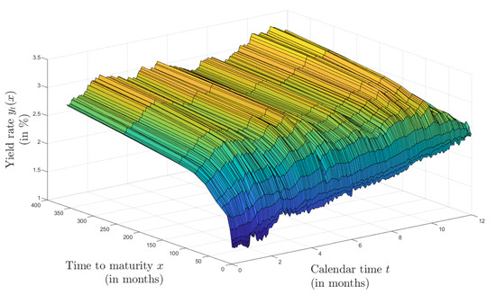
Figure 1. Historical yield rate curves for 2018.

Employing Musiela’s notation [5], let $y_t\left(x\right)$ denote the yield rate of a US treasury traded at time t with the time to maturity x. According to ([4], Definition 3.13), $y_t\left(x\right)$ can be expressed with the aid of the instantaneous forward rate $f_t\left(x\right)$ as

$$y_t\left(x\right)=\frac{1}{x}{\int }_0^x{f}_t\left(x\right)\mathrm{d}x\equiv \frac{1}{x}{\mathcal{I}}_x\left(f_t\right).$$

(15)

In particular, invoking the mean value theorem, the former equation suggests

$$y_t\left(0\right)=f_t\left(0\right)\equiv r_t,$$

(16)

where $r_t$ stands for the short rate. Multiplying both sides of Equation (15) by x and differentiating in x, we can solve for $f_t\left(x\right)$, i.e.,

$$f_t\left(x\right)={\partial }_x\left(x{y}_t\left(x\right)\right)=y_t\left(x\right)+x{\partial }_x{y}_t\left(x\right).$$

(17)

Unfortunately, no “natural” boundary condition is readily available for $f_t\left(x\right)$. In contrast, since $y_t\left(x\right)$ can be assumed bounded in $x=0$, a homogeneneous Dirichlet boundary condition emerges for $x{y}_t\left(x\right)$. Therefore, in spirit of ([4], Chapter 3.3), we will rather work with the (observable) quantity

$$Y(t,x)=x{y}_t\left(x\right),$$

(18)

referred to as the “integrated forward rate” since

$$Y(t,x)={\mathcal{I}}_x\left(f_t\right)\equiv {\int }_0^x{f}_t\left(\eta \right)\mathrm{d}\eta .$$

This quantity, $Y(t,x)$, satisfies the homogeneous Dirichlet boundary condition $Y(t,0)=0$ at $x=0$.

Since the shortest time-to-maturity available in our dataset is $x_{\min }=1$ month, $y_t\left(0\right)$ will be approximated/extrapolated as $y_t\left(x_{\min }\right)$. Further, as Figure 1 suggests, the x-grid becomes very coarse for $x>3\mathrm{years}(=36\mathrm{month})$. In particular, this means that the infinitesimal effects of the operator A in the abstract HJM model in Equation (13) will become negligible as the semigroup $S_t(·)$ will practically “collapse” to the identity operator, essentially reducing the model (for large x) to the classic HJM model. Therefore, the maturities were truncated at 36 months. Lastly, the observed yield rates are interpolated onto $[0,36]$ month using cubic splines. Figure 2 displays the historical Y-curves for the year 2018 over the truncated 36-month x-horizon.

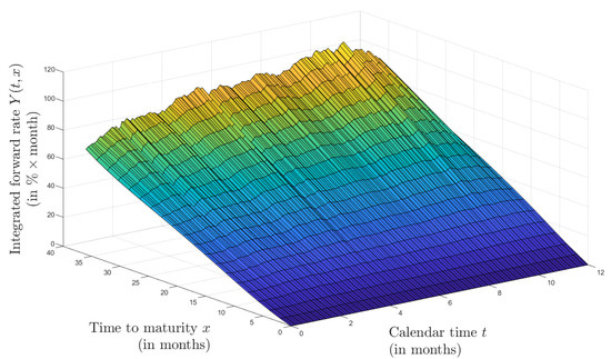
Figure 2. Historical values for integrated forward rates $Y(t,x).$

5.1. The Model

Consider the space ${\mathcal{H}}_w$ defined in Section 4.2. The “spatio-”temporal evolution of the forward rates will be assumed to follow the linear autonomous HJM model from Equation (4), i.e.,

$$\left\{\begin{array}{ccc}\hfill \mathrm{d}{f}_t\left(x\right)& =& (\frac{\mathrm{d}}{\mathrm{d}x}{f}_t\left(x\right)+{\tilde{\alpha }}_t\left(x\right))\mathrm{d}t+{\sum }_{k=1}^{\infty }{\sigma }^k\left(x\right)·\mathrm{d}{\tilde{W}}_k\left(t\right),\hfill \\ \hfill f_0\left(x\right)& =& f^0\left(x\right),\hfill \end{array}\right.$$

(19)

with some initial datum $f^0$ and ${\tilde{\alpha }}_t\left(x\right)$ determined via the “no arbitrage” condition

$$\begin{array}{c}\hfill \tilde{\alpha }\left(x\right)=\sum _{k=1}^{\infty }{\sigma }^k\left(x\right)\left({\int }_0^x{\sigma }^k\left(\eta \right)\mathrm{d}\eta \right),\end{array}$$

where the evolution in Equation (19) is taking place under the risk-neutral measure $\tilde{\mathbb{P}}$. To assure the model is identifiable, similar to [8,10], ${\sigma }^k\left(x\right)$’s will be assumed orthogonal with respect to an appropriate inner product to be discussed later.

Following the results of Section 4, we can write

$${\tilde{W}}_t^k=W_t^k+{\int }_0^t{\lambda }_s^k\mathrm{d}s$$

for a standard cylindircal Wiener process ${\left(W_t\right)}_{t\ge 0}$ with respect to the physical measure $\mathbb{P}$, where ${\left({\lambda }_t\right)}_{t\ge 0}$ must satisfy the conditions of Theorem 3. See also ([10], Section 2). In the spirit of [8], assuming an “affine specification” for the market price of risk

$${\lambda }_t^k\equiv \left({\int }_0^x{\sigma }^k\left(\eta \right)\mathrm{d}\eta \right){\lambda }^k \mathrm{with} \mathrm{some} \mathrm{constant} {\lambda }^k\prime \mathrm{s}$$

the former conditions are trivially satisfied. Thus, Equation (19) can be equivalently expressed under the physical measure $\mathbb{P}$:

$$\left\{\begin{array}{ccc}\hfill \mathrm{d}{f}_t\left(x\right)& =& (\frac{\mathrm{d}}{\mathrm{d}x}{f}_t\left(x\right)+\alpha \left(x\right))\mathrm{d}t+{\sum }_{k=1}^{\infty }{\sigma }^k\left(x\right)·\mathrm{d}{W}_k\left(t\right),\hfill \\ \hfill f_0\left(x\right)& =& f^0\left(x\right),\hfill \end{array}\right.$$

(20)

with

$$\begin{array}{c}\hfill \alpha \left(x\right)={\displaystyle \sum }_{k=1}^{\infty }{\sigma }^k\left(x\right)\left({\int }_0^x{\sigma }^k\left(x\right)\mathrm{d}s+{\lambda }_t^k\right)={\displaystyle \sum }_{k=1}^{\infty }(1+{\lambda }^k){\sigma }^k\left(x\right)\left({\int }_0^x{\sigma }^k\left(x\right)\mathrm{d}s\right).\end{array}$$

Since the parameter vectors ${\left({\sigma }^k\left(x\right)\right)}_{k\in \mathbb{N}}$ and ${\left({\lambda }^k\right)}_{k\in \mathbb{N}}$ are infinite-dimensional, the model (20), though being linear and autonomous, is genuinely non-parametric from the statistical point of view.

Arguing similar to ([4], p. 42), the stochastic process ${\left(Y(t,x)\right)}_{t\ge 0}$ is expected to solve the SPDE:

$$\left\{\begin{array}{ccc}\hfill \mathrm{d}Y(t,x)& =& \left(-\left(\frac{\partial }{\partial x}Y(t,x)-r_t\right)+\frac{1}{2}{\sum }_{k=1}^{\infty }(1+{\lambda }_k){\left({\mathcal{I}}_x{\sigma }^k\right)}^2\left(x\right)\right)\mathrm{d}t\hfill \\ \hfill & & +{\sum }_{k=1}^{\infty }\left({\mathcal{I}}_x{\sigma }^k\right)\left(x\right)·\mathrm{d}{W}_k\left(t\right) \mathrm{for} t>0,x\in (0,x_{\max }),\hfill \\ \hfill Y(t,0)& =& 0 \mathrm{for} t>0,\hfill \\ \hfill Y(0,x)& =& x{y}^0\left(x\right) \mathrm{for} x\in [0,x_{\max }],\hfill \end{array}\right.$$

(21)

where $y^0$ is the initial value for the yield curve $y_t(·)$ at $t=0$ and

$$r_t=f_t\left(0\right)\equiv y_t\left(0\right)$$

denotes the short rate. We would like to draw the reader’s attention to the minus sign in front of the first term on the right-hand side of the first equation in (21). Since the boundary condition is now prescribed at $x=0$, the information propagates from left to right, i.e., the abstract operator is now $A=-\frac{\partial }{\partial x}$ subject to homogeneneous Dirichlet boundary conditions at $x=0$.

On the strength of Hille & Yosida theorem, the operator A with the maximal domain

$$D\left(A\right)=\left\{Y\in \mathcal{H} | AY\in \mathcal{H}, Y(0)=0\right\}$$

(note that the point evaluation is well-defined in view of Sobolev embedding theorem) generates a strongly continuous semigroup ${\left(S_t\right)}_{t\ge 0}$ of contractions on

$$\mathcal{H}=L^2(0,x_{\max };\mathbb{R})$$

endowed with the standard scalar product. The semigroup ${\left(S_t\right)}_{t\ge 0}$ is now the right-shift semigroup given as

$$\left(S_{t}Y\right)\left(x\right)=\left\{\begin{array}{cc}0,& 0\le x\le t\le x_{\max },\\ Y(x-t),& 0\le t\le x\le x_{\max }.\end{array}\right.$$

Assuming $r_t$ is a scalar Itô process independent of the cylindircal Wiener process ${\left(W\left(t\right)\right)}_{t\ge 0}$, the concept of a mild solution can be developed similar to Section 3.1.

To make Equation (21) useful for prediction purposes, we need to specify the evolution of $r_t$. To this end, we utilize the classical Vasiček’s short rate model [37]:

$$\left\{\begin{array}{ccc}\hfill \mathrm{d}{r}_t& =& \alpha ({\tilde{r}}^{*}-r_t)\mathrm{d}t+\beta \mathrm{d}{\tilde{W}}_t^0 \mathrm{for} t>0,\hfill \\ \hfill r_0& =& r^0,\hfill \end{array}\right.$$

(22)

where $\alpha ,\beta ,{\tilde{r}}^{*}>0$ are parameters, $r_0$ is a given random variable independent of ${\left({\tilde{W}}^0\left(t\right)\right)}_{t\ge 0}$ and ${\left({\tilde{W}}^0\left(t\right)\right)}_{t\ge 0}$ is, in turn, independent of $y^0$ and ${\left(\tilde{W}\left(t\right)\right)}_{t\ge 0}$. Since the evolution in Equation (22) is taking place under the risk-neutral measure ${\tilde{\mathbb{P}}}^0$, we perform a change of measures using Girsanov’s theorem assuming

$${\tilde{W}}_t^0=W_t^0+{\int }_0^t{\lambda }^0\mathrm{d}s=W_t^0+{\lambda }^{0}t.$$

Thus, under the physical measure ${\mathbb{P}}^0$, the evolution in Equation (22) assumes the form

$$\left\{\begin{array}{ccc}\hfill \mathrm{d}{r}_t& =& \alpha (r^{*}-r_t)\mathrm{d}t+\beta \mathrm{d}{W}_t^0 \mathrm{for} t>0,\hfill \\ \hfill r_0& =& r^0\hfill \end{array}\right.$$

(23)

with $r^{*}={\tilde{r}}^{*}+\frac{{\lambda }^0}{\alpha }$ and a standard Wiener process ${\left(W_t^0\right)}_{t\ge 0}$. In the following, we will work with Equations (21) and (23) under the physical measures $\mathbb{P}$ and ${\mathbb{P}}^0$. The key feature of Equations (21) and (23) is that they are autonomous, which is crucial requirement if a model is to be used in forecasting.

Since our dataset is discrete, it is natural to discretize Equations (21) and (23) as well. To this end, we employ (semi-)implicit and explicit Euler & Maruyama schemes for time integration and a two-point finite-difference difference quotient approximation for A. Selecting a time grid $\{t_j | j=0,\cdots ,m-1\}$ and a “space” grid $\{x_i | i=0,\cdots ,n-1\}$ with $t_j=j(\Delta t)$, $x_i=i(\Delta x)$, $\Delta t=\frac{T_{\max }}{m-1}$, $\Delta x=\frac{x_{\max }}{n-1}$, we obtain

$$\left\{\begin{array}{ccc}\hfill \frac{Y(t_{j+1},x_i)-Y(t_j,x_i)}{\Delta t}& =& \left(-\left(\frac{Y(t_{j+1},x_{i+1})-Y(t_{j+1},x_i)}{\Delta x}-r_{t_j}\right)+\frac{1}{2}{\sum }_{k=1}^{\infty }(1+{\lambda }^k){\left({\mathcal{I}}_{x_i}{\sigma }^k\right)}^2\left(x_i\right)\right)\hfill \\ \hfill & & +{\sum }_{k=1}^{\infty }\left({\mathcal{I}}_x{\sigma }^k\right)\left(x_i\right)\frac{W_k\left(t_{j+1}\right)-W_k\left(t_j\right)}{\Delta t}\hfill \\ \hfill & & \mathrm{for} j=0,\cdots ,m-2, i=0,\cdots ,n-2,\hfill \\ \hfill Y(t_j,0)& =& 0 \mathrm{for} j=0,\cdots ,m-1,\hfill \\ \hfill Y(t_0,x_i)& =& x_i{y}^0\left(x_i\right) \mathrm{for} i=0,\cdots ,n-1\hfill \end{array}\right.$$

(24)

and

$$\left\{\begin{array}{ccc}\hfill \frac{r_{t_{j+1}}-r_{t_j}}{\Delta t}& =& \alpha \left(r^{*}-r_{t_j}\right)+\beta \frac{W_{t_{j+1}}^0-W_{t_j}^0}{\Delta t} \mathrm{for} j=0,\cdots ,m-2,\hfill \\ \hfill r_{t_0}& =& r^0.\hfill \end{array}\right.$$

(25)

Using standard results from numerical analysis of S(P)DEs, both numerical schemes can be proved to be unconditionally feasible and stable (i.e., for any $\Delta t,\Delta x>0$). The consistency also holds true, but is irrelevant for our purposes as $\Delta t,\Delta x$ remain fixed. A numerical implementation in Matlab^® is given in the Supplementary Materials.

The historical yield rate dataset [7] used in this paper contains $m=249$ time perios for the year 2018. Restricting the times to maturity to 0 to 12 months, the equidistant x-grid contains $n=769$ nodes ranging from 0 to 32 months. Thus, $\Delta t=\frac{12}{m-1}=0.0484$ and $\Delta x=\frac{32}{n-1}=0.0417$.

5.2. Parameter Estimation

Before the model in Equations (24) and (25) can be used for prediction purposes, the unknown functional parameter vector $\sigma \equiv {\left({\sigma }_k(·)\right)}_{j\in \mathbb{N}}$ and the scalar parameters $\alpha ,\beta$ need to be estimated. Since $\sigma$ is infinite-dimensional, the underlying estimation problem is a genuinely non-parametric and will be regularized through a type of PCA (Principal Component Analysis) truncation ([6], Chapter 1.7.1). In the PDE optimization literature, this approach is commonly known as POD (Proper Orthogonal Decomposition) and used as a dimension reduction technique [41].

We begin with Equation (25). The maximum likelihood (ML) estimators for $\alpha ,r^{*}$ and $\beta$ are given as

$$\begin{array}{cc}\hfill \widehat{\alpha }& =-\frac{1}{\Delta t}\log \left(\frac{m{\sum }_{j=1}^m{r}_{t_j}{r}_{t_{j-1}}-\left({\sum }_{j=1}^m{r}_{t_j}\right)\left({\sum }_{j=1}^m{r}_{t_{j-1}}\right)}{m{\sum }_{j=1}^m{R}_{t_{j-1}}^2-{\left({\sum }_{j=1}^m{r}_{t_{j-1}}\right)}^2}\right),\hfill \\ \hfill {\widehat{r}}^{*}& =\frac{1}{m\left(1-\exp (-\widehat{\alpha }\Delta t)\right)}\left({\displaystyle \sum }_{j=1}^m{r}_{t_j}-\exp (\widehat{\alpha }\Delta t){\displaystyle \sum }_{j=1}^m{r}_{t_{j-1}}\right),\hfill \\ \hfill {\widehat{\beta }}^2& =\frac{2\widehat{\alpha }}{m\left(1-\exp (-2\widehat{\alpha }\Delta t)\right)}{\displaystyle \sum }_{j=1}^m{\left(r_{t_j}-r_{t_{j-1}}\exp (-\widehat{\alpha }\Delta t)-\widehat{r}\left(1-\exp (-\widehat{\alpha }\Delta t)\right)\right)}^2\hfill \end{array}$$

(cf. [42,43,44]). The ML estimates for the 2018 historic data are displayed in Table 1 below.

Table 1. ML estimates for the Vasicek model based on 2018 historic short rate data.

$\widehat{\mathit{\alpha }}$	${\widehat{\mathit{r}}}^{*}$	$\widehat{\mathit{\beta }}$
0.079473	−0.63952	0.15449

Since no maximum likelihood estimator is known for $\sigma$ in Equation (24), we will develop a custom least-squares-like method instead. To this end, we rewrite Equation (24) as

$$\left\{\begin{array}{ccc}\hfill V_{t_j}& =& \frac{1}{2}{\sum }_{k=1}^{\infty }(1+{\lambda }^k){\left({\mathcal{I}}_{x_i}{\sigma }^k\right)}^2\left(x_i\right)+{\sum }_{k=1}^{\infty }\left({\mathcal{I}}_x{\sigma }^k\right)\left(x_i\right)\frac{W_k\left(t_{j+1}\right)-W_k\left(t_j\right)}{\Delta t}\hfill \\ \hfill & & \mathrm{for} j=0,\cdots ,m-2, i=0,\cdots ,n-2,\hfill \\ \hfill Y(t_j,0)& =& 0 \mathrm{for} j=0,\cdots ,m-1,\hfill \\ \hfill Y(t_0,x_i)& =& x_i{y}^0\left(x_i\right) \mathrm{for} i=0,\cdots ,n-1\hfill \end{array}\right.$$

(26)

with

$$V_{t_j}=\frac{Y(t_{j+1},x_i)-Y(t_j,x_i)}{\Delta t}+\left(\frac{Y(t_{j+1},x_{i+1})-Y(t_{j+1},x_i)}{\Delta x}-r_{t_j}\right).$$

According to Equation (26), $V_{t_j}$’s are i.i.d. Gaussian elements of $\mathcal{H}$. In view of the fact that we interested in predicting the yields $y_t\left(x\right)$ given as $y_t\left(x\right)=\frac{1}{x}Y(t,x)$, for regularization purposes, we will rather employ the stronger topology of $D\left(A\right)$.

As mentioned before, to render ${\sigma }^k\left(x\right)$’s identifiable, we assume the latter are orthogonal in $\mathcal{H}$. This implies ${\mathcal{I}}_x{\sigma }^k$ are orthogonal in $D\left(\mathcal{A}\right)$ since

$${⟨{\sigma }^k,{\sigma }^l⟩}_{\mathcal{H}}={⟨A{\mathcal{I}}_x{\sigma }^k,A{\mathcal{I}}_x{\sigma }^l⟩}_{\mathcal{H}}={⟨{\mathcal{I}}_x{\sigma }^k,{\mathcal{I}}_x{\sigma }^l⟩}_{\mathcal{D}\left(\mathcal{A}\right)}.$$

(27)

Also note that ${\left({\mathcal{I}}_x\sigma \right)}^2\in \mathcal{H}$ since ${\mathcal{I}}_x{\sigma }^k\in D\left(A\right)\hookrightarrow L^{\infty }\left((0,x_{\max })\right)$ for ${\sigma }^k\in \mathcal{H}$ on the stength of Sobolev’s imbedding theorem and Hölder’s inequality.

We proceed by forming the sample $\{A^{\Delta x}V\left(t_0\right),\cdots ,A^{\Delta x}V\left(t_{m-2}\right)\}$ with the discretized negative derivative operator

$$A^{\Delta x}=-\frac{1}{\Delta x}\left(\begin{array}{ccccccc}1& 0& 0& \cdots & 0& 0& 0\\ -1& 1& 0& \cdots & 0& 0& 0\\ 0& -1& 1& \cdots & 0& 0& 0\\ ⋮& ⋮& ⋮& \ddots & ⋮& ⋮& ⋮\\ 0& 0& 0& \cdots & 1& 0& 0\\ 0& 0& 0& \cdots & -1& 1& 0\\ 0& 0& 0& \cdots & 0& -1& 1\end{array}\right)$$

and compute the covariance operator in the scalar product of

$${\mathcal{H}}^{\Delta x}=\left\{Y=(Y_{t_1},\cdots ,Y_{t_{m-1}}\right\} \mathrm{with} {\parallel Y\parallel }_{{\mathcal{H}}^{\Delta x}}^2=(\Delta x)\sum _{i=1}^{m-1}{Y}^2\left(x_i\right).$$

Let $C^{\Delta x}$ denote the resulting (bounded) covariance operator/matrix given as

$$C^{\Delta x}=\frac{1}{m-2}\sum _{j=0}^{m-1}\left(A^{\Delta x}V\left(t_j\right)-m^{\Delta x}\right)\otimes \left(A^{\Delta x}V\left(t_j\right)-m^{\Delta x}\right)$$

with the sample mean element/vector

$$m^{\Delta x}=\frac{1}{m-1}\sum _{j=0}^{m-2}{A}^{\Delta x}V\left(t_m\right),$$

(28)

Performing spectral decomposition

$$C^{\Delta x}=\sum _{k=1}^p{\nu }_k\left({\varphi }_k\otimes {\varphi }_k\right)$$

for some “principal variances” ${\nu }_1\ge {\nu }_2\ge \cdots \ge {\nu }_p\ge 0$ and unit ${\varphi }_k\in {\mathcal{H}}^{\Delta x}$ (cf. [6], Chapter 1.7.1), we choose the first $p^{\prime }\le p$ “principal modes” responsible for, say, 99% of variation, i.e., we choose the smallest $p^{\prime }$ such that $\frac{{\sum }_{k=1}^{p^{\prime }}{\nu }_k}{{\sum }_{k=1}^p{\nu }_k}\ge 0.99$.

This truncation step, in addition to the $D\left(A\right)$-topology employed, renders the procedure numerically and statistically well-posed. Figure 3 displays the six principal modes responsible for 99.32% of variation in $AV\left(t_j\right)$’s for the 2018 integrated forward rate data. Summarizing, ${\mathcal{I}}_x{\sigma }^k$’s and, thus, ${\sigma }^k$ can now be estimated via

$$\begin{array}{cc}\hfill {\widehat{{\mathcal{I}}_x\sigma }}^k& =\left\{\begin{array}{cc}(\Delta t){\nu }_k^{1/2}{\mathcal{I}}^{\Delta x}{\varphi }_k,& 1\le k\le p^{\prime },\\ 0,& k>p^{\prime }\end{array}\right. {and} \hfill \\ \hfill {\widehat{\sigma }}^k& =\left\{\begin{array}{cc}(\Delta t){\nu }_k^{1/2}{\varphi }_k,& 1\le k\le p^{\prime },\\ 0,& k>p^{\prime },\end{array}\right.\hfill \end{array}$$

(29)

where the discrete negative antiderivative operator

$$-{\mathcal{I}}^{\Delta x}:Y\mapsto {\left(-(\Delta x)\sum _{l=0}^{i}Y\left(t_l\right)\right)}_{i=0,\cdots ,n-1}$$

(30)

comprises the (isometric isomorphic) inverse of $A^{\Delta x}$. Since the covariance operator $C^{\Delta x}$ is (in general) non-spherical, we expect that our method is consistent, but does not necessarily need to exhibit optimal efficiency. The latter can be improved with a type of “backfitting” procedure, which is beyond the scope of this article.

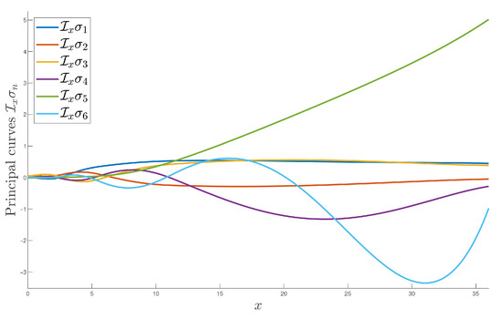
Figure 3. Six principal modes responsible for over 99% of variation.

Once ${\sigma }^k\left(x\right)$’s are estimated, we can estimate ${\lambda }_k$’s using the least squares method. Computing the “design matrix”

$$X^{\Delta x}=\left(A^{\Delta x}\widehat{{\mathcal{I}}_x{\sigma }^1},\cdots ,A^{\Delta x}\widehat{{\mathcal{I}}_x{\sigma }^{p^{\prime }}}\right)$$

and recalling the sample mean $m^{\Delta x}$ from Equation (28), the Gauss & Markov theorem yields an estimate for the “truncated” $\lambda$ vector:

$$\widehat{\lambda }=2{\left({\left(X^{\Delta x}\right)}^{\prime }{X}^{\Delta x}\right)}^{-1/2}{\left(X^{\Delta x}\right)}^{\prime }{m}^{\Delta x}-1.$$

(Note that we first estimated $\frac{1}{2}({\lambda }^k-1)$ and then solved for ${\lambda }^k$.) Applied to the 2018 data, the estimates for the $p^{\prime }=6$ “principal” ${\lambda }^k$’s in given in Table 2.

Table 2. Least-squares estimates for the first $p^{\prime }=6$ parameteres ${\lambda }^k.$

${\widehat{\mathit{\lambda }}}^1$	${\widehat{\mathit{\lambda }}}^2$	${\widehat{\mathit{\lambda }}}^3$	${\widehat{\mathit{\lambda }}}^4$	${\widehat{\mathit{\lambda }}}^5$	${\widehat{\mathit{\lambda }}}^6$
−0.71078	6.88	0.48587	−0.74969	−0.73313	−0.84993

5.3. Prediction

Now, that the estimates $\widehat{\alpha },{\widehat{r}}^{*},\widehat{\beta }$ and ${\widehat{\sigma }}^k,{\widehat{\lambda }}^k$ are at hand, Equations (24) and (25) can be used to predict the dynamics of $r_t$ and $Y(t,x)$ and, thus, that of $y_t\left(x\right)=\frac{Y(t,x)}{x}$. 1 January 2019 was used as $t=0$ with the yield curve from 31 December 2018 (multiplied by x) playing the role of the initial value. We generated $10,000$ sample paths for the standard Wiener increments ${\left(W^k\left(t_{j+1}\right)-W^k\left(t_j\right)\right)}_{0\le j\le m^{\prime }-2,1\le k\le 6}$ and ${\left(W^0\left(t_{j+1}\right)-W^k\left(t_j\right)\right)}_{0\le j\le m^{\prime }-2}$. Here, we chose $m^{\prime }=22$ which corresponds to predicting the integrated forward rates over a one-month time horizon. Further, $10,000$ sample paths of the discretized solution processes $r^{\Delta t,\Delta x,l}, Y^{\Delta t,\Delta x,l}$, $l=1,\cdots ,10,000$ were computed by solving the difference Equations (24) and (25). The predicted yield curves were then formed as $y_{t_j}^{\Delta t,\Delta x,l}\left(x_i\right)=x_i{Y}^{\Delta t,\Delta x,l}$.

To empirically assess the statistical performance of our method, we chose $t=$ 1 February 2020 and compared our predicted curves with the historically observed one. Figure 4 displays the observed yield rate curve (solid) and the estimated mean yield curve ${\overline{y}}_{t_j}^{\Delta t,\Delta x,l}\left(x_i\right)=\frac{1}{10,000}{\sum }_{l=1}^{10,000}{y}_{t_j}^{\Delta t,\Delta x,l}\left(x_i\right)$ (dotted). Further, the dashed curves represent the lower and upper 99% pointwise prediction bounds. Note that the overall confidence level of the resulting tube region is less than 99% since no Bonferroni correction was performed. Figure 4 further contains 5 sample solution paths, which are all (essentially) contained in the prediction region. The estimated mean yield curve is also contained in the prediction region and does not substantially deviate from the observed curve. The prediction region is relatively tight suggesting good predictive power of our model.

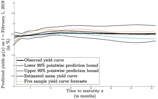
Figure 4. Predicting the yield rates on 1 February 2019 based on 2018 historical data.

The left panel of Figure 5 displays the historical yield curve rates for January 2019 (22 business days), while the right panel gives the estimated mean yield curve rate for the same time window based on $10,000$ replications. We conjecture that the slight overestimation of the yield curve for large maturities may be related with the non-decreasing behavior of the long rates (see Section 4.1).

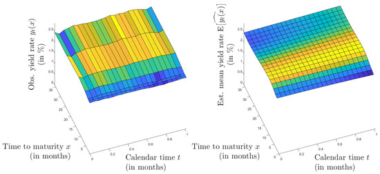
Figure 5. Observed yield curve rates (left) and estimated mean yield curve rates (right) for January 2019.

In sum, the presented model can be used both for prediction and estimation purposes as well as uncertainty quantification. Further potential applications include stochastic optimization and optimal stopping time problems, etc. The full set of Matlab^® codes used to produce the results of Section 5 are available at https://github.com/mpokojovy/abstract.HJM.

6. Discussion and Conclusions

High level of abstraction and numerous prerequisites in various areas of probability theory, stochastic processes and martingale theory, functional analysis and operator semigroup theory, etc., are among the barriers encountered by researchers and practitioners when working with the abstract Heath-Jarrow-Morton (HJM) framework. We attempted to alleviate these difficulties by giving an accessible self-contained review of mathematical results related to the abstract HJM model. Based on real data, we also demonstrated how an infinite-dimensional HJM model can be callibrated and applied to forecasting US Treasury yield curve rates. Our future work will include empirical investigation of the nonlinear models as well as analysis of multiple zero coupon bonds.

Appendix A.1. Representation of Q-Wiener Process

Definition A1

(Q-Wiener process). Let $\mathcal{U}$ be a Hilbert space and $Q\in \mathcal{L}\left(\mathcal{U}\right)$ be symmetric, non-negative and with finite trace. A $\mathcal{U}$-valued stochastic process ${\left(W\left(t\right)\right)}_{t\in [0,T]}$ on a probability space $(\mathsf{\Omega },\mathcal{F},\mathbb{P})$ is called a Q-Wiener process if

• $W\left(0\right)=0$,
• $W\left(t\right)$ has continuous trajectories $\mathbb{P}$-almost surely,
• $W\left(t\right)$ has independent increments, e.g., the random variables $W\left(t_1\right)$, $W\left(t_2\right)-W\left(t_1\right),·,W\left(t_n\right)-W\left(t_{n-1}\right)$ are independent for all $0\le t_1<t_2<\dots <t_n\le T$ and $n\in \mathbb{N}$,
• The increments have Gaussian laws, e.g., $\left(W\left(t\right)-W\left(s\right)\right)\sim \mathcal{N}\left(0,(t-s)Q\right)$ for all $0\le s\le t\le T$.

Proposition A1

(Representation of Q-Wiener process). Let $Q\in \mathcal{L}\left(\mathcal{U}\right)$ be symmetric, non-negative and with finite trace.

Let ${\left\{e_k\right\}}_{k\in \mathbb{N}}$ denote an orthonormal basis of $\mathcal{U}$ comprised of eigenvectors of Q associated with eigenvalues ${\left({\lambda }_k\right)}_{k\in \mathbb{N}}$. For a stochastic $\mathcal{U}$-valued process ${\left(W\left(t\right)\right)}_{t\in [0,T]}$ to be Q-Wiener process, it is necessary and sufficient that

$$\begin{array}{c}\hfill W\left(t\right)=\sum _{k\in \mathbb{N}}\sqrt{{\lambda }_k}{\beta }_k\left(t\right)e_k \mathit{for} \mathit{all} t\in [0,T],\end{array}$$

where ${\left\{{\beta }_k\right\}}_{k\in \mathbb{N}}$ is a vector of independent real-valued Brownian motions with respect to a probability space $(\mathsf{\Omega },\mathcal{F},\mathbb{P})$. The latter series is convergent in the topology of $L^2\left((\mathsf{\Omega },\mathcal{F},\mathbb{P});C\left(\right[0,T],\mathcal{U})\right)$.

Appendix A.2. Q-Wiener Process with Respect to Filtration

Definition A2

(Filtration). Let $T\in [0,\infty )$. A filtration on a probability space $(\mathsf{\Omega },\mathcal{F},\mathbb{P})$ is a family of σ-algebras ${\left\{{\mathcal{F}}_t\right\}}_{t\in [0,T]}$ with the property ${\mathcal{F}}_s\subset {\mathcal{F}}_t\subset \mathcal{F}$ for all $0\le s\le t\le T$.

Definition A3

(Adapted process). A stochastic process ${\left(X\left(t\right)\right)}_{t\in [0,T]}$ is said to be adapted to a filtration ${\left\{{\mathcal{F}}_t\right\}}_{t\in [0,T]}$ if for every $t\in [0,T]$ the random variable $X_t$ is ${\mathcal{F}}_t$-measurable.

Definition A4

(Q-Wiener process). A stochastic process ${\left(W\left(t\right)\right)}_{t\in [0,T]}$ satisfying

• ${\left(W\left(t\right)\right)}_{t\in [0,T]}$ is adapted to ${\left\{{\mathcal{F}}_t\right\}}_{t\in [0,T]}$,
• the increments $W\left(t\right)-W\left(s\right)$ are independent of ${\mathcal{F}}_s$ for all $0\le s\le t\le T$

is referred to as a Q-Wiener process.

Proposition A2.

Let $(\mathsf{\Omega },\mathcal{F},\mathbb{P})$ be a probability space. Any $\mathcal{U}$-valued Q-Wiener process ${\left(W\left(t\right)\right)}_{t\in [0,T]}$ is a Q-Wiener process with respect to the normal filtration ${\left\{{\mathcal{F}}_t\right\}}_{t\in [0,T]}$.

Appendix C.1. Cylindrical Q-Wiener Process

Definition A7

(Cylindrical Q-Wiener process). Let Q be a linear bounded operator, but not necessarily with finite trace, on a Hilbert space $\mathcal{U}$. We call ${\left(W\left(t\right)\right)}_{t\in [0,T]}$ a cylindrical Q-Wiener process over $\mathcal{U}$ if

$$\begin{array}{c}\hfill W\left(t\right)=\sum _{k\in \mathbb{N}}{\lambda }_k^{\frac{1}{2}}{\beta }_k\left(t\right)e_k,\end{array}$$

where ${\left\{{\left({\beta }_k\left(t\right)\right)}_{t\in [0,T]}\right\}}_{k\in \mathbb{N}}$ is a family of independent Brownian motions, ${\left\{{\lambda }_k\right\}}_{k\in \mathbb{N}}$ is a set of eigenvalues of Q with corresponding eigenvectors ${\left\{e_k\right\}}_{k\in \mathbb{N}}$ which form a basis in $\mathcal{U}$. If $Q=I$, ${\left(W\left(t\right)\right)}_{t\in [0,T]}$ is called a standard cylindrical Wiener process.

Since this series may not converge in $L^2((\mathsf{\Omega },\mathcal{F},\mathbb{P});\mathcal{U})$ if Q has no finite trace, we will use the following propositions.

Proposition A6.

Let Q be a linear bounded operator, but not necessarily with finite trace, on a Hilbert space $\mathcal{U}$. Let ${\mathcal{U}}_1$ be a Hilbert space such that there exists a Hilbert-Schmidt embedding $\mathcal{J}:{\mathcal{U}}_0:=Q^{\frac{1}{2}}\left(\mathcal{U}\right)\to {\mathcal{U}}_1$. If ${\left\{e_k\right\}}_{k\in \mathbb{N}}$ is an orthonormal basis of ${\mathcal{U}}_0$ and ${\left\{{\left({\beta }_k\left(t\right)\right)}_{t\in [0,T]}\right\}}_{k\in \mathbb{N}}$ is a family of independent real-valued Brownian motions, then there exists $Q_1\in \mathcal{L}\left({\mathcal{U}}_1\right)$ symmetric, non-negative and with finite trace such that the series

$$\begin{array}{c}\hfill W\left(t\right)=\sum _{k\in \mathbb{N}}{\beta }_k\left(t\right)\mathcal{J}\left(e_k\right) \mathit{for} \mathit{all} t\in [0,T],\end{array}$$

converges in ${\parallel ·\parallel }_{{\mathcal{M}}_T^2\left({\mathcal{U}}_1\right)}={\left\{\mathbb{E}\left({\sup }_{t\in [0,T]}{\parallel (·)\left(t\right)\parallel }_{{\mathcal{U}}_1}^2\right)\right\}}^{\frac{1}{2}}$ and defines a $Q_1$-Wiener process on ${\mathcal{U}}_1$.

Appendix C.2. Integration for Predictable Processes

Definition A8

(Hilbert-Schmidt operator). Given an orthonormal basis ${\left\{e_k\right\}}_{k\in \mathbb{N}}$ of $\mathcal{U}$, we refer to an operator $A\in \mathcal{L}(\mathcal{U},\mathcal{H})$ as a Hilbert-Schmidt operator if

$$\begin{array}{c}\hfill \sum _{k\in \mathbb{N}}{⟨A{e}_k,A{e}_k⟩}_{\mathcal{H}}<\infty .\end{array}$$

The space of all Hilbert-Schmidt operators from $\mathcal{U}$ to $\mathcal{H}$ will be denoted by ${\mathcal{L}}_{\mathrm{HS}}(\mathcal{U},\mathcal{H})$.

Definition A9

(Elementary process). Let T be positive. A stochastic process ${\left(\mathsf{\Phi }\left(t\right)\right)}_{t\in [0,T]}$ is said to be an elementary process on a Hilbert space $\mathcal{U}$ if there is a finite family of disjoint intervals

$$\begin{array}{c}\hfill (s_k,t_k]\subset [0,T],k\in \{1,2,\cdots ,n\} for some n\in \mathbb{N}, {\displaystyle \bigcup }_{k=}^n(s_k,t_k]=(0,T],\end{array}$$

and a corresponding finite family of ${\mathcal{F}}_{s_k}$-measurable random variables ${\left\{{\mathsf{\Phi }}_k\right\}}_{k\in \{1,2,\dots ,n\}}$ taking a finite number of values in the space of Hilbert-Schmidt operators ${\mathcal{L}}_{\mathrm{HS}}(\mathcal{U},\mathcal{H})$ such that for all $t\in [0,T]$

$$\begin{array}{c}\hfill \mathsf{\Phi }(t,\omega )=\sum _{k=1}^n{\mathsf{\Phi }}_k\left(\omega \right)·{\mathbb{1}}_{(s_k,t_k]}\left(t\right) \mathbb{P}-almost surely.\end{array}$$

Definition A10

(Stochastic integral for elementary process). For a given elementary process $\mathsf{\Phi }\in L^2\left([0,T]\times \mathsf{\Omega },{\mathcal{L}}_{\mathrm{HS}}(\mathcal{U},\mathcal{H})\right)$ the stochastic integral is defined by

$$\begin{array}{c}\hfill {\int }_0^T\mathsf{\Phi }\left(t\right)\mathrm{d}W\left(t\right)=\sum _{k=1}^n{\mathsf{\Phi }}_k\left(W\left(t_k\right)-W\left(s_k\right)\right) for some n\in \mathbb{N},\end{array}$$

where ${\left(W\left(t\right)\right)}_{t\in [0,T]}$ is a standard cylindrical $\mathcal{U}$-valued Wiener process.

Definition A11

(Predictable $\sigma$-algebra). A σ-algebra over $[0,T]\times \mathsf{\Omega }$ generated by all subsets of the form $(s,t]\times A,A\in {\mathcal{F}}_s$ with $\left\{0\right\}\times A_0$ for $A_0\in {\mathcal{F}}_0$ is called a predictable σ-algebra and is denoted by ${\mathcal{P}}_T$.

Definition A12

(Predictable process). A stochastic process ${\left(X\left(t\right)\right)}_{t\ge 0}$ with values in a Hilbert space $\mathcal{U}$ is called predictable if it is ${\mathcal{P}}_T$-measurable.

Proposition A7.

The stochastic integral can be uniquely defined for every predictable process $\mathsf{\Phi }\in L^2\left([0,T]\times \mathsf{\Omega },{\mathcal{L}}_{\mathrm{HS}}(\mathcal{U},\mathcal{H})\right)$.

Definition A13

(${\mathcal{F}}_t$-stopping time). An ${\mathcal{F}}_t$-stopping time is a non-negative real-valued random variable τ such that for all times $t\ge 0$ the event $\{\tau \le t\}\in {\mathcal{F}}_t$.

Definition A14

(Simple ${\mathcal{F}}_t$-stopping time). An ${\mathcal{F}}_t$-stopping time τ is said to be simple if it takes only a finite number of values.

Theorem A1

(Itô isometry). If ${\left(\mathsf{\Phi }\left(t\right)\right)}_{t\in [0,T]}\in L^2([0,T]\times \mathsf{\Omega },{\mathcal{L}}_{\mathrm{HS}}(\mathcal{U},\mathcal{H}))$ is predictable and ${\left(W\left(t\right)\right)}_{t\in [0,T]}$ is a standard $\mathcal{U}$-valued cylindrical Wiener process, then we have

$$\begin{array}{c}\hfill \mathbb{E}\left({∥{\int }_0^T\mathsf{\Phi }\left(s\right)\mathrm{d}W\left(s\right)∥}_{\mathcal{H}}^2\right)=\mathbb{E}\left({\int }_0^T{\parallel \mathsf{\Phi }\left(s\right)\parallel }_{{\mathcal{L}}_{\mathrm{HS}}(\mathcal{U},\mathcal{H})}^2\mathrm{d}s\right)=\mathbb{E}\left({\int }_0^T\mathcal{tr}\left({\mathsf{\Phi }}^{*}\left(s\right)\mathsf{\Phi }\left(s\right)\right)ds\right).\end{array}$$

Proposition A8.

Let ${\left(\mathsf{\Phi }\left(t\right)\right)}_{t\in [0,T]}\in L^2([0,T]\times \mathsf{\Omega }, {\mathcal{L}}_{\mathrm{HS}}(\mathcal{U},\mathcal{H}))$ be predictable, ${\left(W\left(t\right)\right)}_{t\in [0,T]}$ be a standard cylindrical $\mathcal{U}$-valued Wiener process and τ be an ${\mathcal{F}}_t$-stopping time such that $\mathbb{P}(\tau \le T)=1$. Then we have $\mathbb{P}$-almost surely

$$\begin{array}{c}\hfill {\int }_0^t\mathsf{\Phi }\left(s\right){\mathbb{1}}_{[0,\tau ]}\left(s\right)\mathrm{d}W\left(s\right)={\int }_0^{\tau \wedge t}\mathsf{\Phi }\left(s\right)\mathrm{d}W\left(s\right).\end{array}$$

Proposition A9.

The stochastic integral defined by

$$\begin{array}{c}\hfill {\int }_0^t\mathsf{\Phi }\left(s\right)\mathrm{d}W\left(s\right):=\underset{n\to \infty }{\lim }{\int }_0^t{\mathbb{1}}_{[0,{\tau }_n]}\left(s\right)\mathsf{\Phi }\left(s\right)\mathrm{d}W\left(s\right) \mathrm{for} \mathrm{all} t\in [0,T]\end{array}$$

does not depend on the choice of the sequence of stopping times ${\left\{{\tau }_n\right\}}_{n\in \mathbb{N}}$ if ${\lim }_{n\nearrow \infty }{\tau }_n=T$.

References

- Heath, D.; Jarrow, R.; Morton, A. Bond Pricing and the Term Structure of Interest Rates: A New Methodology for Contingent Claims Valuation. Econometrica 1992, 60, 77–105. [Google Scholar] [CrossRef]
- Brigo, D.; Mercurio, F. Interest Rate Models—Theory and Practice: With Smile, Inflation and Credit, 2nd ed.; Springer: Berlin/Heidelberg, Germany, 2006. [Google Scholar]
- Harrison, J.; Pliska, S. Martingales and Stochastic Integrals in the Theory of Continuous Trading. Stoch. Proc. Appl. 1981, 11, 215–260. [Google Scholar] [CrossRef]
- Filipović, D. Consistency Problems for HJM Interest Rate Models. Ph.D. Thesis, Swiss Federal Institute of Technology, Zurich, Switzerland, 2001. [Google Scholar]
- Musiela, M. Stochastic PDEs and Term Structure Models. In Journées Internationales de Finance; IGR-AFFI: La Baule, France, 1993. [Google Scholar]
- Carmona, R.; Tehranchi, M. Interest Rate Models: An Infinite Dimensional Stochastic Analysis Perspective, 1st ed.; Springer: Berlin/Heidelberg, Germany, 2006. [Google Scholar]
- US Department of the Treasury. Daily Treasury Yield Curve Rates. Available online: https://www.treasury.gov/resource-center/data-chart-center/interest-rates/Pages/TextView.aspx?data=yield (accessed on 14 April 2020).
- Dai, Q.; Singleton, K. Specification analysis of affine term structure models. J. Financ. 2000, 55, 1943–1978. [Google Scholar] [CrossRef]
- Duffee, G. Term premia and interest rate forecasts in affine models. J. Financ. 2002, 57, 405–443. [Google Scholar] [CrossRef]
- Cheridito, P.; Filipović, D.; Kimmel, R. Market price of risk specifications for affine models: Theory and evidence. J. Financ. Econ. 2007, 83, 123–170. [Google Scholar] [CrossRef]
- Da Prato, G.; Zabczyk, J. Stochastic Equations in Infinite Dimensions, 2nd ed.; Cambridge University Press: New York, NY, USA, 1992. [Google Scholar]
- Reed, M.; Simon, B. Methods of Modern Mathematical Physics, 1st ed.; Academic Press Inc.: Cambridge, MA, USA, 1972. [Google Scholar]
- Capinski, M.; Kopp, E. Measure, Integral and Probability, 2nd ed.; Springer Undergraduate Mathematics Series; Springer: Berlin/Heidelberg, Germany, 2007. [Google Scholar]
- Rudin, W. Functional Analysis, 2nd ed.; International Series in Pure and Applied Mathematics; McGraw-Hill: New York, NY, USA, 1991. [Google Scholar]
- Knoche, C.; Frieler, K. Solutions of Stochastic Differential Equations in Infinite Dimensional Hilbert Spaces and Their Dependence on Initial Data. Ph.D. Thesis, University of Bielefeld, Bielefeld, Germany, 2001. [Google Scholar]
- Björk, T. Arbitrage Theory in Continuous Time, 4th ed.; Oxford Finance Series; Oxford University Press: Oxford, UK, 2020. [Google Scholar]
- Cheyette, O. Interest Rates Models. In Investment Management for Insurers; Babbel, D., Fabozzi, F., Eds.; Frank J. Fabozzi Associates: New Hope, PA, USA, 1999. [Google Scholar]
- Kamizono, K.; Kariya, T. An implementation of the HJM model with application to Japanese interest futures. Financ. Eng. Jpn. Market. 1996, 3, 151–170. [Google Scholar] [CrossRef]
- Sabelli, C.; Pioppi, M.; Sitzia, L.; Bormetti, G. Multi-curve HJM modelling for risk management. Quant. Financ. 2018, 18, 563–590. [Google Scholar] [CrossRef]
- Fernando, W. American Options Pricing Using HJM Approach. Ph.D. Thesis, UNC Charlotte, Charlotte, NC, USA, 2017. [Google Scholar]
- Schmidt, T. An infinite factor model for credit risk. Int. J. Theor. Appl. Financ. 2006, 9, 43–68. [Google Scholar] [CrossRef]
- Babbel, D.; Fabozzi, F. Investment Management for Insurers; Babbel, D., Fabozzi, F., Frank, J., Eds.; Fabozzi Associates: New Hope, PA, USA, 1999. [Google Scholar]
- Miron, P.; Swannell, P. Pricing and Hedging Swaps, 1st ed.; Euromoney Publications PLC. Nestor House, Playhouse Yard: London, UK, 1992. [Google Scholar]
- Black, F.; Scholes, M. The Pricing of Options and Corporate Liabilities. J. Pol. Econ. 1973, 81, 637–654. [Google Scholar] [CrossRef]
- Harrison, J.; Kreps, D. Martingales and arbitrage in multiperiod securities markets. J. Econ. Theor. 1979, 20, 381–408. [Google Scholar] [CrossRef]
- Delbaen, F.; Schachermayer, W. The Mathematics of Arbitrage, 1st ed.; Springer: Berlin/Heidelberg, Germany, 2006. [Google Scholar]
- Dybvig, P.H.; Ingersoll, J.E.; Ross, S.A. Long forward and zero-coupon rates can never fall. J. Bus. 1996, 59, 1–25. [Google Scholar] [CrossRef]
- Brezis, H. Analyse Fonctionnelle, 4th ed.; Thèorie et Applications (French) [Theory and Applications]; Masson: Paris, France, 1993. [Google Scholar]
- Bhar, R.; Chiarella, C. The estimation of the Heath-Jarrow-Morton model by use of Kalman filtering techniques. In Computational Approaches to Economic Problems; Springer: Boston, MA, USA, 1997; pp. 113–126. [Google Scholar] [CrossRef]
- Pang, K. Calibration of Gaussian Heath, Jarrow and Morton and random field interest rate term structure models. Rev. Derivat. Res. 1998, 2, 315–345. [Google Scholar] [CrossRef]
- Jeffrey, A.; Kristensen, D.; Linton, O.; Nguyen, T.; Phillips, P.C. Nonparametric estimation of a multifactor Heath-Jarrow-Morton model: An integrated approach. J. Financ. Econom. 2004, 2, 251–289. [Google Scholar] [CrossRef]
- Broszkiewicz-Suwaj, E.; Weron, A. Calibration of the multi-factor HJM model for energy market. Acta Phys. Polonica B 2006, 37, 1455–1466. [Google Scholar]
- Bhar, R.; Chiarella, C.; Tô, T.D. A Maximum Likelihood Approach to Estimation of a Class of the Heath-Jarrow-Morton Models. Available online: https://econpapers.repec.org/paper/utsrpaper/80.htm (accessed on 28 October 2020).
- Falcò, L.N.; Nave, J. On the calibration of a Gaussian Heath-Jarrow-Morton model using consistent forward rate curves. Quant. Financ. 2011, 11, 495–504. [Google Scholar] [CrossRef]
- Li, S.; Dong, Y. Parametric estimation in the Vasicek-type model driven by sub-fractional Brownian motion. Algorithms 2018, 11, 197. [Google Scholar] [CrossRef]
- Funahashi, H. An approximate swaption formula in Heath-Jarrow-Morton models. J. Derivat. 2020, 27, 1–21. [Google Scholar] [CrossRef]
- Vasicek, O. An equilibrium characterization of the term structure. J. Financ. Econom. 1977, 5, 177–188. [Google Scholar] [CrossRef]
- Dörsek, P.; Teichmann, D. Efficient simulation and calibration of general HJM models by splitting schemes. SIAM J. Financ. Math. 2013, 4, 575–598. [Google Scholar] [CrossRef][Green Version]
- Kluge, W. Time-Inhomogeneous Lévy Processes in Interest Rate and Credit Risk Models. Ph.D. Thesis, University of Freiburg, Freiburg, Germany, 2005. [Google Scholar]
- Kim, S.; Pokojovy, M.; Wan, X. The taut string approach to statistical inverse problems: Theory and applications. J. Comput. Appl. Math. 2021, 382, 113098. [Google Scholar] [CrossRef]
- Sachs, E.W.; Volkwein, S. POD-Galerkin approximations in PDE-constrained optimization. GAMM-Mitteilungen 2010, 33, 194–208. [Google Scholar] [CrossRef]
- Tang, C.; Chen, S. Parameter estimation and bias correction for diffusion processes. J. Econom. 2009, 149, 65–81. [Google Scholar] [CrossRef]
- Fergusson, K.; Platen, E. Application of maximum likelihood esitmation stochastic shortrate models. Ann. Financ. Econom. 2015, 10, 1–26. [Google Scholar]
- Ballestra, L.; Pacelli, G.; Radi, D. A note on Fergusson and Platen: “Application of maximum likelihood estimation stochastic short-rate models”. Ann. Financ. Econom. 2016, 11, 1–7. [Google Scholar] [CrossRef]
Publisher’s Note: MDPI stays neutral with regard to jurisdictional claims in published maps and institutional affiliations. |
© 2021 by the authors. Licensee MDPI, Basel, Switzerland. This article is an open access article distributed under the terms and conditions of the Creative Commons Attribution (CC BY) license (http://creativecommons.org/licenses/by/4.0/).