Abstract
The proportional–integral plus Clegg integrator (PI + CI) controller is a hybrid extension of the proportional–integral (PI) controller that is able to overcome fundamental limitations of the linear and time-invariant control systems, potentially obtaining faster responses without increasing overshooting. This work focused on the analysis and design of PI + CI controllers and reset controllers in general, for the case of parallel multiple-input single-output (MISO) systems, extending previous design methods developed for the single-input single-output (SISO) case. Several design strategies were developed: one for first-order MISO plants achieving a flat response with a finite settling time, and for second-order MISO plants obtaining a fast response with a reduced overshoot and settling time in comparison with non-hybrid strategies. Several case studies were also developed to illustrate the potential of the proposed methods.
1. Notation
is the n-dimensional Euclidean space. The transpose of a matrix A will be denoted by . A vector or matrix whose elements are vectors or matrices denotes their concatenation. I and 0 denote, respectively, the identity and zero matrices, where the dimensions are clear from context. The notation denotes the ordinary Euclidean norm. The symbol ← is used for assignments or redefinitions. For a subset , denotes its interior and its closure. The symbol × denotes the Cartesian product. A sequence of vectors is denoted by , and , with a free index i, which will sometimes be used to refer to the entire sequence when the context is clear.
A continuous function belongs to class (denoted ) if it is strictly increasing and unbounded, and . If the unboundedness condition is dropped, it is said that f belongs to class . For a hybrid arc , denotes its associated hybrid time domain.
2. Introduction
Linear time-invariant (LTI) control systems are known to come unavoidably associated with fundamental limitations on their performance [1]. This fact motivates the interest in nonlinear control strategies such as hybrid strategies (a hybrid system is a system whose time evolution can be both continuous and discrete), capable of potentially overcoming these limitations, while remaining simple to understand and implement.
Reset control systems [2] form an important class of hybrid control systems. Conceptually, reset control is a type of hybrid control in which controllers come equipped with mechanisms for (fully or partially) resetting their state according to a given triggering event, such as reaching a predefined threshold, or at prescribed time intervals. The field of reset control has proven fruitful in the single variable setting, with a multitude of reset strategies having been successfully devised and applied in the case of single-input single-output (SISO) systems. However, the problem of deriving reset control strategies for multiple input and/or multiple output (MIMO) systems remains comparatively less explored, with only a few works specifically dealing with this case [3,4,5,6,7].
One specific class of MIMO systems is that of multiple-input single-output (MISO) systems. An interesting property of these systems is the availability of multiple control signals which are able to act together on a single output, allowing for the possibility of collaborative control strategies where the controllers may share the control load, with the aim of improving closed-loop performance and robustness or reducing the cost of feedback with respect to SISO strategies. In the process industry, one can find an example of applications of these systems, e.g., in the control of heat exchangers, distillation columns or chemical reactors [8,9,10]. More recent innovative applications of MISO control can be found, e.g., in the field of microfluidics, specifically in the control of two-phase microfluidic processes [11]. More specifically, this work is focused on the parallel MISO control structure, one of two main classes of control structure for MISO systems usually considered in the literature [8,9,12].
A fundamental example of a reset controller, now called the Clegg integrator (CI), was introduced by Clegg in their seminal work [13]. The CI can be thought of as an integrator whose internal state is reset when its input signal passes through zero. Any general reset controller can be built using Clegg integrators together with linear integrators and constant gains, in the same way that the general linear controller can be built using only linear integrators and constant gains. In particular, the proportional–integral plus Clegg integrator (PI + CI) controller [14] consists of a parallel interconnection of a proportional–integral (PI) controller and a Clegg integrator. More specifically, the integral part is replaced by a weighted linear combination of a linear integrator and a CI, where the weight is a new dimensionless design parameter , called the reset ratio. Intuitively, when the controller input signal crosses zero, its averaged state (defined as the weighted averaged sum of the states of the integrator and of the CI) is scaled by a factor of , corresponding to a partial resetting. Between consecutive reset actions, the behavior of the PI + CI controller is that of a linear PI controller (base controller), with all its familiar properties.
In this work, we consider a robust implementation of the Clegg integrator in the framework of hybrid inclusions (HI) [15], by attaching a zero-crossing detection mechanism [16] to it, and also considering other improvements such as a variable band resetting law and variable reset ratio. A parallel MISO control structure is considered, for which both well-posedness and stability in the framework of [15] will be analyzed.
Several design methods for PI + CI tuning are proposed for reference tracking and disturbance rejection. These design methods allow to achieve perfect tracking and disturbance rejection in the case of the parallel control of first-order plants, and an improved response based on the optimization of a weighted integrated squared error (ISE) in the case of higher-order plants.
This work is a revised and extended version of the conference paper [17], where new contributions include an extension to high-order plants of the design rules for the first-order MISO plants therein derived, as well as an analysis of stability and well-posedness. In Section 3, we recall some basic definitions and results of the HI framework, also introducing respective models for the CI, the PI + CI, and general reset controllers, considering different resetting laws. Section 4 discusses the proposed parallel MISO reset control structure, including some simple stability conditions for later use. In Section 5, first-order MISO plants are investigated, and design techniques to achieve a flat response, both in reference tracking and disturbance rejection, are derived. Similarly, Section 6 is devoted to higher-order MISO plants, for which a design technique is obtained for the proper tuning of PI + CI controllers with variable reset. Several case studies are also presented to illustrate the developed design techniques.
3. Preliminaries
3.1. The HI Framework
This work uses the hybrid dynamical systems framework (usually referred to as the hybrid inclusions framework) developed in [15]. Some basic definitions follow (see [15] for technical details), specifically adapted to a particular class of hybrid system with jump and flow maps given by continuous functions. A hybrid system with state is given by
with the following data: the flow mapping , the jump mapping , the flow set , and the jump set .
A hybrid time domain E is a subset of , it is an union of intervals of the form for any and some nondecreasing sequence of real numbers (finite or infinite), with the last interval (if it exists) possibly being of the form , with T finite or . A solution to the hybrid system is a function (or hybrid arc) defined on a hybrid time domain and taking values on , which is locally absolutely continuous on each interval of E. Any solution must satisfy:
- almost everywhere when its image is contained in ; and
- when its image is in .
Moreover, it must satisfy .
For , the so-called hybrid basic conditions [15] are satisfied if f and g are continuous functions, and the sets and are both closed subsets of . It can be shown that these conditions guarantee that is well-posed; informally speaking, the limit of any graphically convergent sequence of solutions to the system is also a solution, even when the system is subject to vanishingly small perturbations (where the graphical convergence of a sequence of hybrid arcs means the convergence of their graphs in ). The well-posedness of a hybrid system implies that its solution sets inherit several relevant properties: upper semicontinuous dependence with respect to initial conditions, robustness against perturbations such as measurement noise and the preservation of asymptotic stability under small perturbations.
A compact set is called locally pre-asymptotically stable for the hybrid system if for every there exists such that any solution to the system with satisfies for any , and if there exists such that any solution satisfying is bounded and, if is complete, .
Note that uniform global pre-asymptotic stability implies local pre-asymptotic stability. A sufficient condition for uniform pre-asymptotic stability is the existence of a Lyapunov function. Assume that satisfies the hybrid basic conditions, and that there exists a candidate Lyapunov function V with , that is continuously differentiable on an open set containing .
A closed set is uniformly globally pre-asymptotically stable for the hybrid system if there exists a candidate Lyapunov function V, and a continuous positive definite function such that the three following conditions are satisfied:
Moreover, a closed set is uniformly globally pre-asymptotically stable for the hybrid system if conditions (2a) and (2b) hold for some V, there exists such that:
and there exist some and such that for any solution to the system, implies:
Note that these stability conditions apply to those instances in which there is a finite number of jumps for a given initial condition.
3.2. Reset Control
A reset controller [18] is a linear and time-invariant (LTI) controller (referred to as a base controller) with a mechanism to fully or partially reset its state to zero, according to some given triggering condition (the resetting law), such as a signal reaching a specified threshold. In this work, both zero-crossing and reset band resetting laws will be used [2,16,19], i.e., a reset is performed when the closed-loop error takes a zero value, or when its magnitude reaches some threshold.
3.2.1. A Clegg Integrator with Zero-Crossing Detection
A basic reset controller is the Clegg integrator (CI) [13], which is a fundamental building block in the structure of a reset controller. Several models of the CI have been used in the literature [2,18,20]. Here, the following recent implementation will be used [16,17]:
where is the CI state, and the jump and flow sets are given by
as illustrated in Figure 1. This implementation, which uses a discrete state q to detect a zero-crossing of the error signal e, has the advantage of being robust against abrupt changes in e due for example to measurement noise.
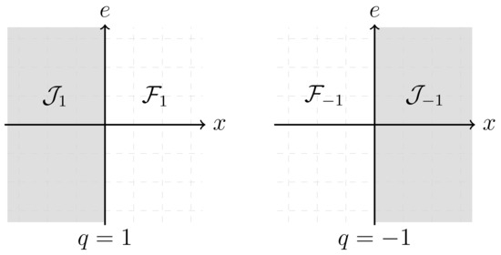
Figure 1.
Jump and flow sets for the zero-crossing resetting law.
3.2.2. The PI + CI Controller
This work is especially focused on the PI + CI controller [14] which is a simple extension of the well-known proportional–integral (PI) controller, to which a CI is added in parallel (Figure 2). In addition to the proportional gain and the integral time , it has one extra parameter , the reset ratio. In spite of its simplicity, the PI + CI controller has been successfully used in several practical applications [2,19].
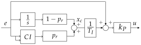
Figure 2.
Block diagram of a proportional–integral plus Clegg integrator (PI + CI) controller.
Its state is , where is composed of two sub-states corresponding to the linear integrator state and the CI state, and is given by
where , and the output signal is:
The jump and flow sets are given by (6) in the case of a zero-crossing resetting law. The case of reset band corresponds to:
where is the output of some (possibly nonlinear) transformation applied to the signal e. If for some , then the controller has a variable band resetting law, and the parameter is the variable band.
In addition, it may be appropriate in control practice to use a time-varying reset ratio [2,19]. In this case, the controller performs a variable reset.
As will be seen in Section 5 and Section 6, the Clegg integrator in the PI + CI controller may be thought of as a substitute of the (filtered) derivative term in the more traditionally used proportional–integral–derivative (PID) controller, fulfilling a similar role with respect to reducing the overshoot and settling time. The similarities become even more prominent once one considers a variable band, which is also essentially a predictive element depending on the derivative of the error. For this reason, although a more general “PID + CI” consisting of a PI + CI plus a derivative term is mathematically possible, it is not considered in this work to avoid unnecessary complexity.
3.2.3. A General Reset Controller
More generally, a reset controller with state , and with a number of states to be reset, is considered. It is assumed that the last states are set to zero at a jump, whereas the other states remain unaffected. The reset controller is described by
where are constant matrices of the appropriate dimensions. Again, the resetting law is given by the flow and jump sets (6) or (9), depending on the case.
4. Reset Control of MISO Systems
MISO systems represent an important class of problems in control practice, which arise whenever two or more control inputs are available to act on a single output. The collaborative control of MISO systems is based on dividing the control effort into multiple controllers acting on each input. In this way, a well-designed MISO control strategy is capable of using the additional control variables to reduce the cost of feedback on the controllers and improve the closed-loop performance with respect to a strategy using only one input (SISO), as well as yielding better robustness in the case of controller saturation or failure [8,9]. Among the examples of MISO systems in the process industry, as mentioned in the introduction, we can find applications in the control of heat exchangers, distillation columns or chemical reactors [8,9,21].
The main goal of this work was the application of reset control to MISO systems, with the basic purpose of obtaining an improved performance. In particular, the focus will be on PI + CI controllers; we will show how they can be applied to the MISO setting, overcoming the performance of the universally used PI(D) controllers. The case of parallel MISO control structures will be investigated in the following.
4.1. Parallel MISO Reset Control Systems
One of the two main MISO control system structures is the parallel control structure (Figure 3), also known as centralized control or load-sharing control (the other main structure is the series control structure). This structure is a generalization of the one proposed in Brosilow et al. [12], and has been considered for example in [8,9,22,23,24]. Applications can be found, e.g., in [25] (idle speed control of an engine), [10] (temperature control), [26] (aero-electric power station control), [27] (control of spacecrafts), [28] (control of a continuous stirred tank reactor) and [29] (control of an artificial pancreas).
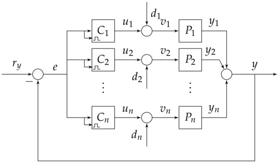
Figure 3.
Block diagram of a parallel multi.input single-output (MISO) control structure.
An LTI MISO system consisting of n plants is controlled by respective reset controllers , , of the form (10). The ith plant is described by
and we will add the subscript i to refer to all variables in (10) associated with the ith controller except the variable q, which will be shared among all of them (this will be referred to as synchronous reset). The total output is defined by . Finally, the feedback connection is achieved by setting , where is a reference signal, and , for input disturbances , for
This kind of MISO control structure has the advantage of being versatile, and is commonly used in cases where there is no clear hierarchical ordering into plants with fast and slow dynamics [9]. Sometimes a master controller is also explicitly considered as part of the structure (this is called coordinated control); however, from a mathematical perspective, it can be treated as part of the other controllers by means of the redefinition .
The closed-loop state is defined as
where, in addition, . For the case of zero exogenous inputs (reference and disturbances), the closed-loop reset control system is then described as a hybrid system similar to (1):
where and are uniquely determined from etc. Namely, A is given by
and by
The resetting law is given by the jump and flow sets
for some matrix (of matrix function) . Note that both and are closed sets whose union is the whole space. The zero-crossing resetting law corresponds to:
whereas it is easy to see that a variable band resetting law, where all controllers have the same variable band , can be equivalently modeled by choosing:
More general resetting laws could be considered in principle, for example, a resetting law in which each controller has its own variable band , but the reset control system analysis and design would be much harder.
Note that setting individual reset actions may cause asynchronous triggering at different times, and this switching-like behavior cannot be captured by a single hyperplane-crossing detection. Another consequence is that sharing the logical variable q among the controllers is not anymore justified; instead, each controller needs to keep its own associated variable , which further complicates the treatment. Furthermore, undefined behavior would arise when the system is in such a state that two or more reset actions are triggered at the same time; one would need to consider cases in total to properly account for all possibilities, corresponding to the number of possible non-empty subsets of controllers affected by a reset. For these reasons, only the case of identical variable bands will be taken into consideration in this work.
4.2. Well-Posedness and Stability
Consider the parallel MISO reset control system , as given by (11)–(15). Well-posedness of directly follows from the fact that and are continuous maps, and the flow and map sets and are closed sets, and thus satisfies basic hybrid conditions. Well-posedness in this sense [15] is a less restrictive condition than the one considered in [30]. Nevertheless, it still implies some important properties regarding the robustness, stability and nature of the solutions (we refer the reader to [15] for technical details).
Stability for the closed-loop system (12) of the set is analyzed in the following. The set consists of the two equilibrium states at zero (one for each value of the variable q). The problem is approached by using a Lyapunov function satisfying the sufficient Lyapunov conditions for to be uniformly globally asymptotically stable for .
(Stability Conditions #1) Consider the parallel MISO reset control system with a zero crossing resetting law. The set is globally asymptotically stable for if there exists a matrix such that:
and:
hold for some and any matrix Θ such that .
Proof.
The MISO reset control system has a state . Consider a quadratic Lyapunov function , the result follows after checking the sufficient Lyapunov conditions (2). Condition (2a) is easily satisfied by taking and where and are, respectively, the minimum and maximum eigenvalues of P, both positive real numbers since . For the condition (2b), it is true that:
now taking , from (18a) directly follows (2b). The fulfillment of condition (2c) is a bit more complicated. Firstly, it is shown that (2c) can be relaxed to:
since no solution to the system (12) takes values in the region except possibly at the initial instant . By contradiction, we assume that there exists some solution such that satisfies (2c) for some , and thus . There are two possibilities:
- , and then . This means that , and we must have both and . However, this is impossible, since and .
- belongs to a connected component of which is not a singleton, i.e., there exists such that for all , and hence for almost all such . Since is an open set, we can choose small enough such that . However, this is a contradiction, since is empty.
For the case of a resetting law with a variable reset band, corresponding to flow and jump sets given by (15) and (17), stability does not follows from (18), since in this case, . However, a more conservative version of this result holds for this resetting law if one replaces (18b) by the more conservative condition:
Note that both conditions in Section 4.2, and the modified condition (21), are stated in the form of linear matrix inequalities (LMI), which is useful for computational purposes.
The following alternative stability conditions easily follow (basically they correspond to the case of a stable base system that performs a finite number of jumps).
(Stability Conditions #2) Consider the parallel MISO reset control system with a zero crossing resetting law. The set is globally asymptotically stable for if there exists a matrix such that (18a) is satisfied, and in addition, there exist some and such that for any solution ϕ to the MISO system, implies:
Proof.
It follows directly since conditions (2a), (2b) and (4) of the stability result are satisfied with a quadratic Lyapunov function . For condition (3), consider a function , where is the largest eigenvalue of and is the smallest eigenvalue of P. □
5. Design of PI + CI Controllers for Parallel First-Order MISO Plants
In this section, we derive two sets of tuning rules that produce a flat response against step disturbances or reference changes, respectively, for first-order systems, extending previous work [31] to parallel MISO control structures. The term “flat response” (see Figure 4) is understood to mean that the error signal is zeroed after the first reset instant, that is, becomes identically zero for all , where denotes the first reset instant. Two different control objectives are considered:
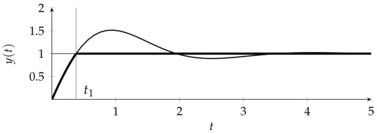
Figure 4.
Illustration of a closed-loop flat response y under a reference change: (thin line) equivalent linear response, (thick line) resetted response.
- Reference tracking: the output signal must asymptotically follow a given reference signal as closely as possible;
- Disturbance rejection: the effect of possible disturbance signals at the input of each plant must be minimized.
Each control objective is treated separately; if in a certain application both control objectives need to be met, one may follow the approach in [31] where the controller allows for time-varying reset ratios, and a supervisory control mechanism is added to detect which disturbance is acting on the system (if any), modifying accordingly.
Taking into account the considered control objectives, the problem can be separated into two independent parts: first, the base linear system’s parameters are tuned to achieve the desired initial speed, and then, the parameters affecting the reset actions are adjusted to reduce the overshooting and settling time after zero-crossings; consequently, any common LTI design strategy can be used to tune and . The developments in this section and the next one concern the latter part.
Consider the first-order linear MISO plant given by the subplants:
In the following developments, it is assumed that the base linear controllers are designed in such a way that the error signal presents oscillatory behavior, crossing zero in finite time (otherwise no reset would take place, and the evolution of the system would be identical to that of its LTI equivalent). This means that the base linear response will usually be more aggressive than that obtained by following some common PI tuning rules such as the Skogestad Internal Model Control (SIMC) rule [32]. However, as we will see, a flat response will always be nominally produced no matter how fast the base dynamics is.
5.1. Reference Tracking
Suppose that a step change in the reference signal is applied to the system into consideration, which we assume to be initialized at zero. Here denotes the Heaviside unit step function, whereas is a scaling factor. Denote by the first reset instant, i.e., the minimum such that . From (7)–(23), the ith plant state flows in according to:
A closer look at the controller states and reveals that:
that is, all the integrator and CI states of all the controllers take an identical constant value (which is defined as with some abuse of notation) before the first jump. After the jump, the integrator states hold their value , and the CI states are reset to zero. Now, since after the first jump it is true that , and , and also and (the jump is produced at the instant in which the error signal is zero), then from (24), the results show that:
It is clear that a flat response will be achieved if for all plants, since in this way the closed-loop system reaches its steady state (as the time derivatives , for ). From (26), it directly follows that the reset ratio takes the value:
As a result, to obtain a flat response y, that is, a response with and for any , each PI + CI controller should have a different reset ratio given by (27), depending on the value of the plant state at the first jump . Moreover, not all the are independent due to the fact that and . In particular, they satisfy:
5.2. Disturbance Rejection
According to the parallel control structure (Figure 3), different disturbances may be acting at the input of the plants . It is again considered that they are step disturbances (for any ). It is assumed that the system is initially at rest.
The flow equation for the state associated to the plant is:
After the first jump, that is, at , again , , , and , and thus (30) results in:
After rearranging terms, the tuning rule for the reset ratio that produce a flat response (making ) is:
where again, since and , reset ratios must satisfy:
5.3. Guidelines and Limitations
The tuning rules for a flat response (27) and (32) depend on values of the plant states after the first jump. In fact, they use the n plant states , but one of them linearly depends on the others through (28) or (33). A reasonable way to obtain the values , without the necessity of using an analytical expression, is by using state observers. Note that since the integrator and CI states of all the controllers are identical up to the first jump, then:
for , and thus it is only strictly necessary to tune the reset ratios just before the first jump at . As a consequence, the controllers have a time interval to obtain a good estimate of . Note that once the reset ratios are tuned at the first jump, then they keep the same value afterwards.
An important fact is that although in (27), (28) and (32), (33) reset ratios values explicitly depend on the amplitudes and of the reference and disturbances, respectively, it turns out that resulting tuned values take the same values independently of and . This is due to the fact that, before the first jump, the MISO reset control system flows like a linear (and time-invariant) system, and thus the values of and scale accordingly to the amplitudes and . The result is that the values are intrinsic numbers of the MISO reset control system for a flat response: the same values will produce flat responses for any step reference or disturbance signal of arbitrary amplitude.
Unlike in the SISO case, where the tuning rules always result in reset ratios between 0 and 1, the MISO tuning rules (27) or (32) (for ) may result in large values of (positive or negative) in some cases. Since the proposed PI + CI controllers are equipped with a zero-crossing detection mechanism (by the use of the discrete state q), this is not a major issue even with (small) measurement noise, since is reasonably bounded when resets occur close to a zero-crossing. Nevertheless, whenever large reset ratios arise in practice, it might be an indication that either the base linear controllers are ill-designed or the plants have very different dynamics (for example, one is much slower than the others). In the latter situation, the PI + CI-based parallel control approach might be unsuitable, and one should consider a different control structure.
5.4. Stability
The proposed parallel control architecture generically includes marginally stable modes for the flow dynamics if . Indeed, consider defined as
for some such that , and any ().
It easily follows that and , and since then there exist solutions to the MISO reset control system with for any , corresponding to alternating flows and jumps of arbitrary length.
As a consequence, some modification is necessary for the PI + CI control strategy to achieve closed loop stability with respect to the equilibrium point . One simple way to avoid this problem is to slightly modify the PI + CI controller structure by including a small damping parameter affecting all the Clegg integrator blocks, as follows:
The presence of the new design parameter makes it impossible to achieve a perfect flat response with a zero-crossing law, since in general . However, a reasonable approximation in practice is obtained for small values of in comparison to the inverse of the closed-loop rise time.
It should be emphasized that in the SISO case [2,14], corresponding to , stability is proven by taking advantage of the fact that the reset instants are always periodic. This special feature is particular to SISO systems (and first-order plants), and it is no longer true in the MISO setting. Non-periodicity makes the stability analysis essentially as difficult as the general case, thus one has to resort to more general results such as the stability conditions developed in Section 4.2.
Since, in a well-tuned MISO reset control system, the error will be very close to its steady state after a finite number of resets (usually 3–5 jumps will suffice), the stability conditions can be directly used by imposing a maximum number of reset actions.
Note that condition (22) is trivially satisfied with J being the maximum number of jumps and . Furthermore, the rest of the conditions are easily satisfied when the base system is stable.
5.5. Case Study: Reference Tracking in a MISO System
Consider a parallel MISO reset control system, with the three plants given by the following transfer functions:
(to connect with previous sections, note that we have ). The base linear PI controllers were initially tuned according to the Skogestad Internal Model Control (SIMC) rule [32] (treating each plant–controller subbranch as an SISO system), and then the values of and were manually modified to produce a dominant oscillatory closed-loop response, thus forcing the reset to occur. The resulting parameters are:
For simplicity, here, the values of and have been obtained by simulating the step response of the MISO reset control system with the base PI controllers, and then obtaining the values of the plant states and integrator states at the first jump (in practice, a state observer should be used). Using: (27) and (28), for , results in:
These reset ratios, jointly with (39), determine the three PI + CI controllers. The unit step response of the MISO reset control system is now simulated, where a measurement noise consisting of a pseudo-random uniform signal of magnitude 0.025 has been added to the plant output. Figure 5 shows the expected flat response after the first jump; noting that, in spite of the measurement noise, the overshooting has been almost completely eliminated in comparison with the base control system, considerably decreasing the settling time as well (the response would be flat after the first jump in absence of noise). It should be emphasized that this property of robustness to noise is formally guaranteed by the fact that the parallel MISO reset control system (12) satisfies the basic hybrid conditions [15]. Note also that the sensor noise effect on the closed-loop systems is similar both for the base and the resetted controllers, and does not significantly degrade the after-reset response, even if the reset action is triggered a little earlier than in the noiseless case.
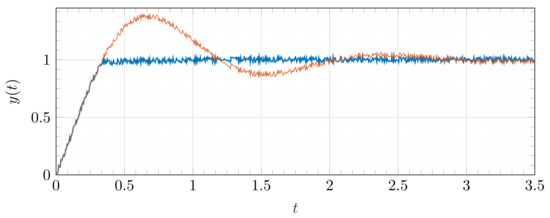
Figure 5.
Closed-loop step response y under a reference change: (orange) base PI controllers; and (blue) PI + CI controllers.
Moreover, the controller outputs are shown in Figure 6a–c, showing how control signals achieve their steady state at the first reset instant. Finally, the closed-loop stability of this MISO reset control system is analyzed. Once the modification (37) is performed on all PI + CI controllers, with , the stability conditions from Section 4.2 are checked to be feasible by using a semidefinite programming solver. The solution:
is obtained, and thus the origin is globally asymptotically stable for the MISO reset control system.
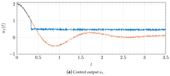
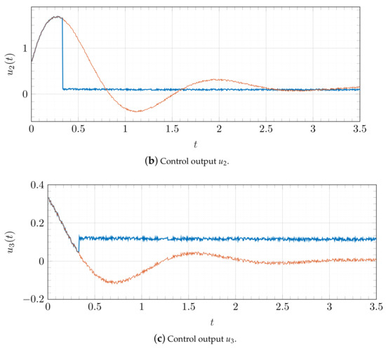
Figure 6.
Controller outputs for the reference tracking example: (orange) base PI controllers; (blue) PI + CI controllers.
Alternatively, by disabling jumps after the first one, stability conditions from Section 4.2 easily apply, since the base MISO system with is stable (which can be easily proven by checking the eigenvalues of A).
5.6. Case Study: Disturbance Rejection in a MISO System
In this example, a disturbance rejection problem with a two-input system is considered, where the two plants are given by the following transfer functions:
The problem of disturbance rejection is considered for step disturbances at the input of the first plant. No measurement noise is explicitly considered in this case, as it has already been shown not to significantly affect the results. The corresponding PI controller parameters, tuned to obtain a fast oscillatory response in the same way as Case Study 5.5, are:
A disturbance is considered (), consisting of the sum of a unit step at and a step of amplitude at . As Figure 7 clearly shows, both disturbances are perfectly rejected by two respective reset actions (it is worth emphasizing that the values of are constant and there is no need to update them after each reset). The controller outputs are shown in Figure 8a,b.
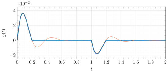
Figure 7.
Closed-loop response y under a disturbance signal: (orange thin line) base PI controllers; (blue thick line) PI + CI controllers.
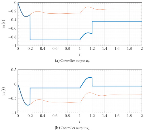
Figure 8.
Controller outputs for the disturbance rejection example: (orange thin line) base PI controllers; (blue thick line) PI + CI controllers.
Now, we consider closed-loop stability for this MISO system. Again, we perform the modification (37) on both PI + CIs, taking a small value such as . As before, solving the LMI stability conditions , the solution:
is found. As a result, the origin is globally asymptotically stable for the MISO reset control system.
Again, if only one jump is allowed, the stability conditions may be used to prove stability by directly checking that the eigenvalues of the matrix A are strictly in the left half plane.
6. Design of PI + CI Controllers for Parallel High-Order MISO Plants
In control practice, it is relatively rare for systems to exhibit only first-order behavior. Many important physical phenomena such as oscillations or resonance are tied to the existence of complex poles in the frequency domain, which requires at least second-order plants. Hence, it is desirable to explore possible extensions of the previously developed PI + CI-based strategies to higher-order systems.
In general, even for the SISO case, the PI + CI controller is unable to achieve a flat response for plants with orders higher than one. It is nevertheless true that the PI + CI may still achieve a good performance in comparison with a PI controller [19]. In the following, this previous PI + CI design method will be extended and improved for the case of a parallel MISO plant, postulating time-varying reset ratios and a variable band resetting law.
6.1. Time-Varying Reset Ratios
A time-varying reset ratio of is postulated. For any , it is considered that constant, for . These values , are computed by minimizing the integrated squared error (ISE) after each reset action, weighted by an exponential term. More specifically, is computed by minimizing the value , defined as
where , , which is what the error signal after the jump would be if no more jumps were enabled. In addition, an exponential weight, with a new parameter , is used to give more weight to the values of the error signals close to the instant .
Note that, as a particular case, when , we recover the method developed in [19]. In general, a good rule of thumb is to take , where denotes the average time interval between two consecutive zero-crossings of the base system; in this way, is an approximation of the integrated squared error between and , since at times , the contribution will be exponentially suppressed. Following the method in [19], and considering the new exponential weighting factor, results in:
Here, is a solution of the Lyapunov equation . As before, we distinguish two cases: reference tracking and disturbance rejection. For each case, it is assumed that the matrix A corresponds to a minimal realization of the base MISO control system.
Since depends affinely on , we arrive at a quadratic minimization problem whose objective function is of the form where . This minimization problem has an explicit solution given by . As a result, the proposed reset ratios for the m PI + CI controllers are simply obtained by
where and are quadratic functions of with coefficients that depend only on the parameters of the plants and controllers.
6.2. A Variable Band Resetting Law
Another degree of freedom to achieve a better performance is based on the modification of the zero-crossing resetting law. Here, the variable band resetting law (17) is proposed, with a parameter that is related to the bandwidth. It is assumed that all the PI + CI controllers are synchronous, i.e., all have the same variable band.
In principle, a good idea would be to consider a time-varying parameter , and compute optimal values by minimizing . However, if , enters the objective function in a rather complex way, which makes it very difficult, if not impossible, to solve the optimization problem. Here, a simple two-step design method is proposed, considering a constant value of :
- A value of is chosen. It must be taken low enough so that the error signal is, to a good approximation, linear in the time intervals spanning units of time before any zero-crossing. In general, if the plants are approximated by first-order systems with time delay, should be taken as smaller than the lowest of the delays.
6.3. Guidelines and Limitations
In general, as in the first-order case, the obtained expression (46) depends on the plant and controller states at . An online implementation of this algorithm requires knowing or estimating the values of the plant states, in real time (this is also true, particularly in the SISO case, where the reset ratio is an explicit function of [19]). Again, in a situation where state feedback is unavailable, a simple way to estimate plant states is to use a state observer and make use of the estimated values etc. Note that this will be more difficult if either the order of the number of plants is high, since a MISO mth order plant has in general a total of states.
An important difference with respect to both the MISO first-order and SISO second-order cases is that no explicit algebraic formula is available to calculate . However, as mentioned previously, it follows from the form of the minimization problem that and , where M and are exclusively functions of the parameters of the plants and base controllers, and thus numerically computable a priori once the plant has been identified. Thus, updating the reset ratios online involves the evaluation of a known quadratic function at a vector , which is not computationally expensive.
Another possible limitation absent from the first-order case concerns the use of the variable band, which depends on the derivative of the error signal. This derivative must be filtered to avoid accidental early triggering of a reset action due to measurement noise. To avoid this problem, a standard solution (also common, e.g., in PID controllers with a nonzero derivative part) is to use a low-pass filter with an associated time constant . According to the frequency analysis performed in [19], if the time filter constant is chosen such that , the filter will reduce the effect of noise without negatively affecting the reset actions.
Finally, the same considerations with regard to reset ratios of high magnitude for the first-order reset strategy in Section 5.3 are also applicable here.
6.4. Case Study: Step Tracking for a Second Order Plant
This case consists of a two-input single-output plant that models a refrigeration system, and has been adapted from [21], where it comprises the cooling part of a room temperature control system. Here, the two plants (corresponding to an air conditioning input and a cooling water input, respectively) are approximated by second-order systems, and the above design method is applied to design a parallel PI + CI control setup. The plants are given by the transfer functions:
The two base PI controllers are first designed for a fast and oscillatory response, following the same method as in previous case studies. Their parameters are:
With these parameters, the dominant complex eigenvalues of the closed loop system are , so the zero-crossings of the base system occur with an eventual semi-period of s. One has ; the slightly higher value is chosen.
Moreover, a variable band should be used, where is the smallest plant delay [21]. After some trial and error, we choose .
Finally, Equation (46) is used for the online computation of the values or , at Here the reference input is a step signal of amplitude starting at . The reset actions have been disabled after three jumps (at s) when the error signal is near the stationary state. As we can see in Figure 9, in comparison with the base control system, the step response is clearly improved after the first reset action at , considerably decreasing both the overshooting and the settling time. The controller outputs are shown in Figure 10a,b, and the (time-varying) reset ratios in Figure 11.
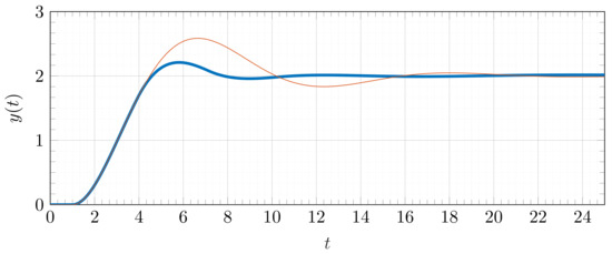
Figure 9.
Closed-loop step response output y: (orange thin line) base PI controllers; (blue thick line) PI + CI controllers.
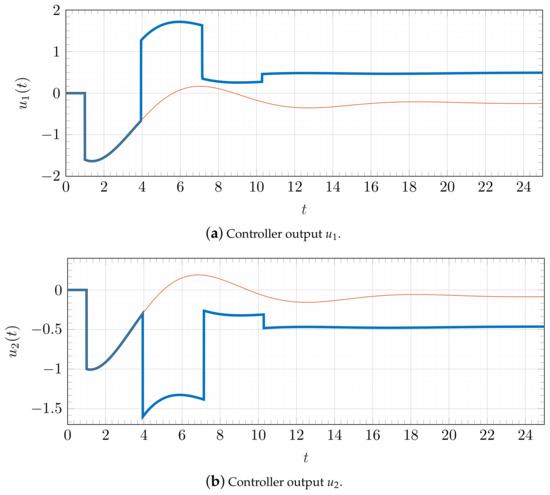
Figure 10.
Controller outputs for the step response: (orange thin line) base PI controllers; (blue thick line) PI + CI controllers.
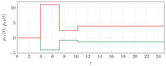
Figure 11.
Projection onto the time domain of the time-varying reset ratios (green) and (red) in the third case study.
Table 1 shows the ISE, IAE and overshoot metrics for the MISO reset control system compared to the base LTI MISO control system; the result is an improvement of of the ISE, of the integrated absolute error (IAE) and of the maximum overshoot percentage. Finally, closed-loop stability easily follows by directly applying the stability conditions , with .

Table 1.
Integrated squared error (ISE), integrated absolute error (IAE), and maximum overshoot percentage, for the parallel MISO reset control system and its base system.
7. Conclusions
New reset control strategies for MISO plants under a parallel configuration have been explored in the framework of hybrid inclusions, in which a model for a general reset controller has been formalized, allowing for the statement and proof of several desirable structural properties such as robustness against measurement noise or stability. The main contributions of this work are a set of design methods to tune reset controllers, specifically PI + CI controllers, which generalize previous design techniques that have been found very useful in the single variable setting to the MISO case.
We considered both first-order MISO plants, where tuning rules were derived achieving a flat closed-loop step response (both in reference tracking and disturbance rejection), and higher-order plants, where an online algorithm has been developed, obtaining an optimal performance minimizing the integral of a weighted squared error. It is believed that this work will also serve as a basis to develop reset control strategies for several other related problems, such as for example a series MISO control structure, as well as MISO plants with time delays.
Author Contributions
Conceptualization, J.F.S. and A.B.; methodology, J.F.S.; software, J.F.S.; formal analysis, J.F.S.; investigation, J.F.S.; writing—original draft preparation, J.F.S.; writing—review and editing, A.B.; supervision, A.B.; project administration, A.B.; funding acquisition, A.B. Both authors have read and agreed to the published version of the manuscript.
Funding
This research was funded by FEDER-European Union and Ministerio de Ciencia e Innovación (Government of Spain) under project DPI2016-79278-C2, and by Fundación Séneca (Comunidad Autónoma de la Región de Murcia) under project 20842/PI/18.
Institutional Review Board Statement
Not applicable.
Informed Consent Statement
Not applicable.
Data Availability Statement
Not applicable.
Conflicts of Interest
The authors declare no conflict of interest.
Abbreviations
The following abbreviations are used in this manuscript:
| PI | Proportional–integral |
| PID | Proportional–integral–derivative |
| CI | Clegg integrator |
| SISO | Single-input single-output |
| MISO | Multiple-input single-output |
| MIMO | Multiple-input multiple-output |
| LTI | Linear time-invariant |
| LMI | Linear matrix inequalities |
| ISE | Integrated squared error |
| IAE | Integrated absolute error |
| HI | Hybrid inclusions |
| SIMC | Skogestad internal model control |
References
- Krishnan, K.; Horowitz, I.M. Synthesis of a nonlinear feedback system with significant plant-ignorance for prescribed system tolerances. Int. J. Control 1974, 19, 689–706. [Google Scholar] [CrossRef]
- Baños, A.; Barreiro, A. Reset Control Systems; Springer: London, UK, 2012. [Google Scholar] [CrossRef]
- Paesa, D.; Franco, C.; Llorente, S.; Lopez-Nicolas, G.; Sagues, C. Reset observers applied to MIMO systems. J. Process. Control 2011, 21, 613–619. [Google Scholar] [CrossRef]
- Yuan, C.; Wu, F. Output feedback reset control of general MIMO LTI systems. In Proceedings of the 2014 European Control Conference (ECC), Strasbourg, France, 24–27 June 2014; pp. 2334–2339. [Google Scholar] [CrossRef]
- Zhao, G.; Hua, C. Discrete-Time MIMO Reset Controller and Its Application to Networked Control Systems. IEEE Trans. Syst. Man Cybern. Syst. 2018, 48, 2485–2494. [Google Scholar] [CrossRef]
- Yazdi, S.; Khayatian, A.; Asemani, M.H. Optimal robust model predictive reset control design for performance improvement of uncertain linear system. ISA Trans. 2020, 107, 78–89. [Google Scholar] [CrossRef]
- Hosseini, I.; Fiacchini, M.; Karimaghaee, P.; Khayatian, A. Optimal reset unknown input observer design for fault and state estimation in a class of nonlinear uncertain systems. J. Frankl. Inst. 2020, 357, 2978–2996. [Google Scholar] [CrossRef]
- Henson, M.A.; Ogunnaike, B.A.; Schwaber, J.S. Habituating control strategies for process control. AIChE J. 1995, 41, 604–618. [Google Scholar] [CrossRef]
- Rico-Azagra, J.; Gil-Martínez, M.; Elso, J. Quantitative feedback control of multiple input single output systems. Math. Probl. Eng. 2014, 2014, 136497. [Google Scholar] [CrossRef] [Green Version]
- Eitelberg, E. Load sharing in a multivariable temperature control system. Control Eng. Pract. 1999, 7, 1369–1377. [Google Scholar] [CrossRef]
- Gagliano, S.; Cairone, F.; Amenta, A.; Bucolo, M. A real time feed forward control of slug flow in microchannels. Energies 2019, 12, 2556. [Google Scholar] [CrossRef] [Green Version]
- Brosilow, C.; Popiel, L.; Matsko, T. Coordinated Control. In Proceedings of the Third International Conference on Chemical Process Control (CPC), Asilomar, CA, USA, 12–17 January 1986; Elsevier: New York, NY, USA, 2020; pp. 295–313. [Google Scholar]
- Clegg, J.C. A nonlinear integrator for servomechanisms. Trans. Am. Inst. Electr. Eng. Part II Appl. Ind. 1958, 77, 41–42. [Google Scholar] [CrossRef]
- Baños, A.; Vidal, A. Design of Reset Control Systems: The PI + CI Compensator. J. Dyn. Syst. Meas. Control 2012, 134, 051003. [Google Scholar] [CrossRef]
- Goebel, R.; Sanfelice, R.G.; Teel, A.R. Hybrid Dynamical Systems: Modeling Stability, and Robustness; Princeton University Press: Princeton, NJ, USA, 2012. [Google Scholar]
- Baños, A.; Barreiro, A. Reset control systems: The zero-crossing resetting law. arXiv 2021, arXiv:2105.13950. [Google Scholar]
- Sáez, J.F.; Baños, A. Tuning Rules for the Design of MISO Reset Control Systems. In Proceedings of the 2020 6th International Conference on Event-Based Control, Communication, and Signal Processing (EBCCSP), Kraków, Poland, 23–25 September 2020; IEEE: New York, NY, USA, 2020; pp. 1–7. [Google Scholar]
- Beker, O.; Hollot, C.; Chait, Y.; Han, H. Fundamental properties of reset control systems. Automatica 2004, 40, 905–915. [Google Scholar] [CrossRef]
- Davó, M. Analysis and Design of Reset Control Systems. Ph.D. Thesis, Universidad de Murcia, Murcia, Spain, 2015. [Google Scholar]
- Zaccarian, L.; Nesic, D.; Teel, A.R. First order reset element and the Clegg integrator revisited. In Proceedings of the 2005, American Control Conference, Portland, OR, USA, 8–10 June 2005; Volume 1, pp. 563–568. [Google Scholar]
- Reyes-Lúa, A.; Skogestad, S. Multi-input single-output control for extending the operating range: Generalized split range control using the baton strategy. J. Process. Control 2020, 91, 1–11. [Google Scholar] [CrossRef]
- Eitelberg, E. Load Sharing Control; NOYB Press: Durban, South Africa, 1999. [Google Scholar]
- Alvarez-Ramirez, J.; Velasco, A.; Fernandez-Anaya, G. A note on the stability of habituating process control. J. Process. Control 2004, 14, 939–945. [Google Scholar] [CrossRef]
- Schroeck, S.J.; Messner, W.C.; McNab, R.J. On compensator design for linear time-invariant dual-input single-output systems. IEEE/ASME Trans. Mechatronics 2001, 6, 50–57. [Google Scholar] [CrossRef]
- Jayasuriya, S.; Franchek, M.A. A QFT-type design methodology for a parallel plant structure and its application in idle speed control. Int. J. Control 1994, 60, 653–670. [Google Scholar] [CrossRef]
- Gutman, P.O.; Horesh, E.; Guetta, R.; Borshchevsky, M. Control of the Aero-Electric Power Station—an exciting QFT application for the 21st century. Int. J. Robust Nonlinear Control IFAC-Affil. J. 2003, 13, 619–636. [Google Scholar] [CrossRef]
- Garcia-Sanz, M.; Hadaegh, F. Load-sharing robust control of spacecraft formations: Deep space and low Earth elliptic orbits. IET Control Theory Appl. 2007, 1, 475–484. [Google Scholar] [CrossRef]
- Velasco-Pérez, A.; Álvarez-Ramírez, J.; Solar-González, R. Multiple input-single output (MISO) control of a CSTR. Revista Mexicana de Ingeniería Química 2011, 10, 321–331. [Google Scholar]
- Moscardó, V.; Díez, J.L.; Bondia, J. Parallel control of an artificial pancreas with coordinated insulin, glucagon, and rescue carbohydrate control actions. J. Diabetes Sci. Technol. 2019, 13, 1026–1034. [Google Scholar] [CrossRef]
- Baños, A.; Mulero, J.I.; Barreiro, A.; Davó, M.A. An impulsive dynamical systems framework for reset control systems. Int. J. Control 2016, 89, 1985. [Google Scholar] [CrossRef] [Green Version]
- Baños, A.; Davó, M.A. Tuning of reset proportional integral compensators with a variable reset ratio and reset band. IET Control Theory Appl. 2014, 8, 1949–1962. [Google Scholar] [CrossRef]
- Skogestad, S. Simple analytic rules for model reduction and PID controller design. J. Process. Control 2003, 13, 291–309. [Google Scholar] [CrossRef] [Green Version]
Publisher’s Note: MDPI stays neutral with regard to jurisdictional claims in published maps and institutional affiliations. |
© 2021 by the authors. Licensee MDPI, Basel, Switzerland. This article is an open access article distributed under the terms and conditions of the Creative Commons Attribution (CC BY) license (https://creativecommons.org/licenses/by/4.0/).