Article

Statistics and Practice on the Trend’s Reversal and Turning Points of Chinese Stock Indices Based on Gann’s Time Theory and Solar Terms Effect

1
College of Science, Beijing Forestry University, Beijing 100083, China
2
School of Information Science & Technology, Beijing Forestry University, Beijing 100083, China
*
Author to whom correspondence should be addressed.
Mathematics 2021, 9(15), 1713; https://doi.org/10.3390/math9151713
Submission received: 2 June 2021 / Revised: 17 July 2021 / Accepted: 18 July 2021 / Published: 21 July 2021
(This article belongs to the Section Probability and Statistics)

Abstract

:
Despite the future price of individual stocks has long been proved to be unpredictable and irregular according to the EMH, the turning points (or the reversal) of the stock indices trend still remain the rules to follow. Therefore, this study mainly aimed to provide investors with new strategies in buying ETFs of the indices, which not only avoided the instability of individual stocks, but were also able to get a high profit within weeks. Famous theories like Gann theory and the Elliott wave theory suggest that as part of the nature, market regulations and economic activities of human beings shall conform to the laws of nature and the operation of the universe. They further refined only the rules related to specific timepoints and the time cycle rather than the traditional analysis of the complex economic and social factors, which is, to some extent, similar to what the Chinese traditional culture proposes: that every impact on and change in the human society is always attributable to changes in the nature. The study found that the turns of the stock indices trend were inevitable at specific timepoints while the strength and intensity of the turns were uncertain, affected by various factors by then, which meant the market was intertwined with both certainty and uncertainty at the same time. The analysis was based on the data of the Shanghai Index, the Second Board Index and the Shenzhen Index, the three major indices that represent almost all aspects of the Chinese stock market, for the past decades. It could effectively reduce the heteroscedasticity, instability and irregularity of time series models by replacing 250 daily high-frequency data with the extreme points near every twenty-four solar terms per year. The forecasts focusing on the future stock trend of the all-solar-terms group and the eight-solar-terms group were proved accurate. What is more, the indices trend was at a high probability to turn in a range of four days at each solar term. The alert period also provided the readers with a practical example of how it works in the real investment environment.

1. Introduction

1.1. General Survey of the Study

According to the efficient-market hypothesis (EMH) and the adaptive market hypothesis (AMH), the future price of an individual stock is impossible to predict and, as the efficiency of the market goes high, the market tends to be more stochastic and disordered, and there are no methods to make any valid prediction ahead from the present. Even though the market is not that efficient in the real world, the prediction is still very hard and unrealistic to make [1].
On the contrary, many researchers have been studying and proved that stock indices are rather predictable to some extent in terms of volatility, revenue, returns, etc. [2,3]. Stock indices are comprehensive special-type stocks that represent a category of individual stocks instead of the stocks belonging to a certain company. Stock indices are more stable and regular and also reflect a country’s overall development of the economy and finance.
Furthermore, our study mainly focused on the turns and reversal of trend of the three major Chinese stock indices (i.e., whether they would rise or fall in the future or fluctuate with no obvious rise or fall but not the forecast of a certain price or point or an analysis of a numeric error).
The three major indices are the Shanghai Index, the Second Board Index and the Shenzhen Index.
There are around 3000 stocks totally in China’s stock market covering all categories of companies and businesses while the three indices are the only three indices that generally represent the 3000 stocks.
The Shanghai Index and the Shenzhen Index cover a range of state-owned companies, big industrial companies, bank securities, energy and resources companies, manufacturing companies, etc. They show the basic power of a country. The Second Board Index includes some startup enterprises, high-technology companies, innovative companies, service industries, environmental protection companies, etc. It shows the advanced technology of China.
Although there are also other smaller indices, they are actually the sub-indices of the three indices above. However, the new Tech Innovation Index only appeared in 2020, so it lacks a great deal of samples.
These three indices are like DJI, IXIC and SPX 500 in the US and therefore we do not need to care about any individual stocks but focus on the three indices.
In general, we selected those three indices that are capable of showing the comprehensive status of China’s stock market. They are all-round and stable, covering all kinds of stock categories.
With the results of indices, we can invest in the ETFs that belong to them which are the Shanghai 50 ETF (510050), the Second Board 50 Fund (159949) and the Shanghai–Shenzhen 300 Fund (000300). Those funds are exactly coincident with the indices they correspondingly belong to. Since the indices are not available to invest, we buy their ETFs. In other words, if the index rises, the ETF rises correspondingly. Figuring out the rule of index reversal can simultaneously reflect on the ETFs, bringing direct financial profit to investors.
The major finding and philosophy of the study is that market rules and economic activities of human beings conform to the laws of nature and the operation of the universe. There are both certainty and uncertainty intertwining in the stock market and, in fact, that also exists in every aspect of the world, and that is the nature philosophy. Nothing remains without changes, like the stock market, but if we figure out when it is possible to have a reversal or what is the signal before turning points, that would be enough for our investment. Therefore, our philosophy in the study was to find out those aspects that will not change apart from the uncertainty.
In this paper, we started with defining the trend and turning points of stocks which many investors only judge by their intuitive feeling or depending on the shape in the software. We first transferred the intuitive feeling to strict definition, and it could be applied in further related studies. We then made a series of statistics to show the correlation between the stock trend and solar terms as well as the probability. We later introduced the concept “alert period” which was actually a practical example to tell the readers how to operate in the real investment environment. We also discussed the EMH and the AMHA in detail, confirming that our study was based on the rationality and feasibility theories. Meanwhile, we explained why time factor was important beyond other regular human factors. In the last part of the study, we used a time series analysis to make further forecast and assessment.
This study mainly took the Shanghai Stock Index (000001) as an example to make a detailed process discovering the relationship between the solar term and the turning points of the index trend, and used the solar term for the time series analysis to predict the future trend.
Meanwhile, we also tested the Second Board Index and the Shenzhen Index as evidence of applicability of our study. However, for convenience, we only show the results of these two indices directly with the same approach as dealing with the Shanghai Index.

1.2. Introduction of Chinese Twenty-Four Solar Terms

The Chinese traditional twenty-four solar terms are the theory and wisdom of natural climate and the turning points of seasons summarized by the ancient Chinese people.
With the arrival of one solar term after another, farming, planting and other agricultural activities also usher in one key timepoint after another. The twenty-four solar terms provide people with crucial time information such as when to sow, when to enhance farming, when to rest and stop farming and when to harvest. Moreover, the temperature and climate of each year also change significantly in these 24 solar terms, forming fluctuations. The seasonal cycle of rising and falling, annual cooling, heating, rainfall and snowfall often occur at a time very close to or exactly at the solar term.
Twenty-four solar terms have been widely used in the field of traditional Chinese medicine [4], which makes us more firmly believe that the natural law represented by the Chinese twenty-four solar terms, as the traditional culture, has already had a potential impact on various aspects of human society [5]. Our study uses the twenty-four solar terms to discover the possible impact on the stock market [6,7].
Today’s twenty-four solar terms are based on the position of the sun on the ecliptic. That’s the annual motion track of the sun which is divided into 24 equal parts, each 15° is one part (Figure 1), each one is a solar term; the first one is Chunfen and the last one is Dahan. On 30 November 2016, the twenty-four solar terms were officially listed in the UNESCO representative works on intangible human cultural heritage.
In the time cycle theory of Gann theory [8], the division of Gann’s wheel and the date or time cycle corresponding to the angle often lead to the turning of stock trend. Gann’s wheel can represent the cycle of one year, ten years or even thirty years, and the division of Gann’s wheel in one year as a cycle is exactly the same as with the 24 solar terms in China, and the most important eight angles also perfectly match the most important eight solar terms in the 24 solar terms.
We were inspired by Gann theory, but we were more willing to propose a Chinese-style method and theory. Therefore, in the following parts of the study, we mainly discussed the relationship between the solar terms and the stock reversal.
Making significant analysis and achievement on solar terms may also inspire other researchers to apply them in other fields, and the philosophy of the time factor is really important in guidance. We reviewed it in the Discussion part of the paper.

1.3. Data

The data we used in Chapter 2 are as follows:
Shanghai Index (code 000001): daily closing price (point) of marketing days from 3 January 1995 to 14 August 2020, 6463 datapoints in total.
Second Board Index (code 399006): daily closing price (point) of marketing days from 1 June 2010 to 9 February 2021, 2693 datapoints in total.
Shenzhen Index (code 399001): daily closing price (point) of marketing days from 3 January 1995 to 3 February 2021, 6439 datapoints in total.
The data we used in Chapter 5 are as follows:
Based on the data above but differently, we only used the price near each solar term which is the biggest n-day extreme point in a 4-day time radius of each solar term.
The last several solar terms were used as the test group.
The data are open and easily found on many websites such as https://money.163.com, accessed on 28 February 2021; readers that are not in China may also download them for free; to find them, enter the stock code.

1.4. Time Cycle Theory and Division of Time

In this section, we introduce an innovated philosophy in stock analysis, which actually was not that new in ancient China, the main refrain throughout our study. The philosophy is that time matters at all times. According to our previous experience and the Chinese traditional culture, human society is affected by natural factors at every moment, and one of the factors is time (including the time cycle, timepoints and time periods).
Despite the fact that the absolute price of a stock is generally supposed to be unpredictable, the turning points and reversal of trend of stock indices have rules to follow. Gann theory [9,10,11,12,13,14] suggests that the cycle of time is almost everywhere in the stock market, like our pulse cycle and four seasons of the year. Nobody denies the existence of the time cycle as it retains its rationality and regularity in the nature. Whether or not we know, the regular shocks and vibrations in the stock market caused by time do happen.
In our paper, we only analyzed the trend and turning points of the Shanghai Index rather than a certain stock or an absolute stock price. We supposed that the index is a wide and general performance of the stock market which eliminates many extreme and irregular cases.
Many theories have focused on calendar effects [15,16,17], and all of them show the effort in searching for the independent time factors over regular human factors that may affect the stock market. However, such a division of time is so modern that the turns do not always falls on them. Besides the solar terms, in China, we have 12 zodiacs (corresponding to a 12-year cycle), lunar months (corresponding to the monthly change of the moon), 10 heavenly stems and 12 earthly branches as well as the constellation of both the Chinese version and the Western version (Figure 2). Thus, we can see that throughout the history, ancient people were always doing tremendous work in summarizing many kinds of time cycles in order to survive, forecast and develop their civilization.
For this reason, we had no need to summarize anything anew. We simply adapted the solar terms of the ancient people and firmly believe that the 24 solar terms are already an effective division of time periods which have potential influences on other aspects of life not only in the agriculture, but also in the stock market, human body, mood, stability of the society, etc. Therefore, in this paper, we made an effort to figure out whether there is a link and correlation between the turning points of the Shanghai Index trend and the solar terms.
Finally, we made an example to explain the concept of time in four-dimensional space as follows:
We say that altitude is not equal to temperature (i.e., it gets colder with height), but imagine a two-dimensional worm being moved up and down by someone else in the air; it may get confused about what makes it feel cold for a while as it is not able to detect that it is actually the change in altitude that causes the change of temperature. Therefore, we, the human beings, also lack the ability to discover the cause in time (i.e., time is a four-dimensional factor that may cause volatility in our three-dimensional world), and we believe that while we are moving ahead along the time axis (t axis), we may come across many specific timepoints that influence certain aspects of our world (e.g., the stock market, investors’ mood, efficiency of the market, world events, etc.); that is the reason why Gann and Elliott both stressed the time cycle, the wave cycle, etc.

2. Turning Point and Extreme Point

2.1. Time Cycle Theory and Division of Time

Definition 1. 
Price (point) of a stock (index).Let the price of a stock per day x = x ( t ) be a function of date.
P.S. Based on the fact that we only focused on indices in this paper, we did not distinguish between the price and the point, the stock and the stock index.
Definition 2. 
Extreme point of range. Extreme point of range   P = P ( n , t ) is an extreme point over n days before and after, t is a date. We call it an n-day extreme point, where n is an integer, i.e.,   t   s . t .   t [ t n , t + n ]
If:
  • x ( t ) < x ( t ) , P + ( n , t ) is a high n-day extreme point;
  • x ( t ) > x ( t ) , P ( n , t ) is a low n-day extreme point.
Usually, we call them both n-day extreme points in brief.
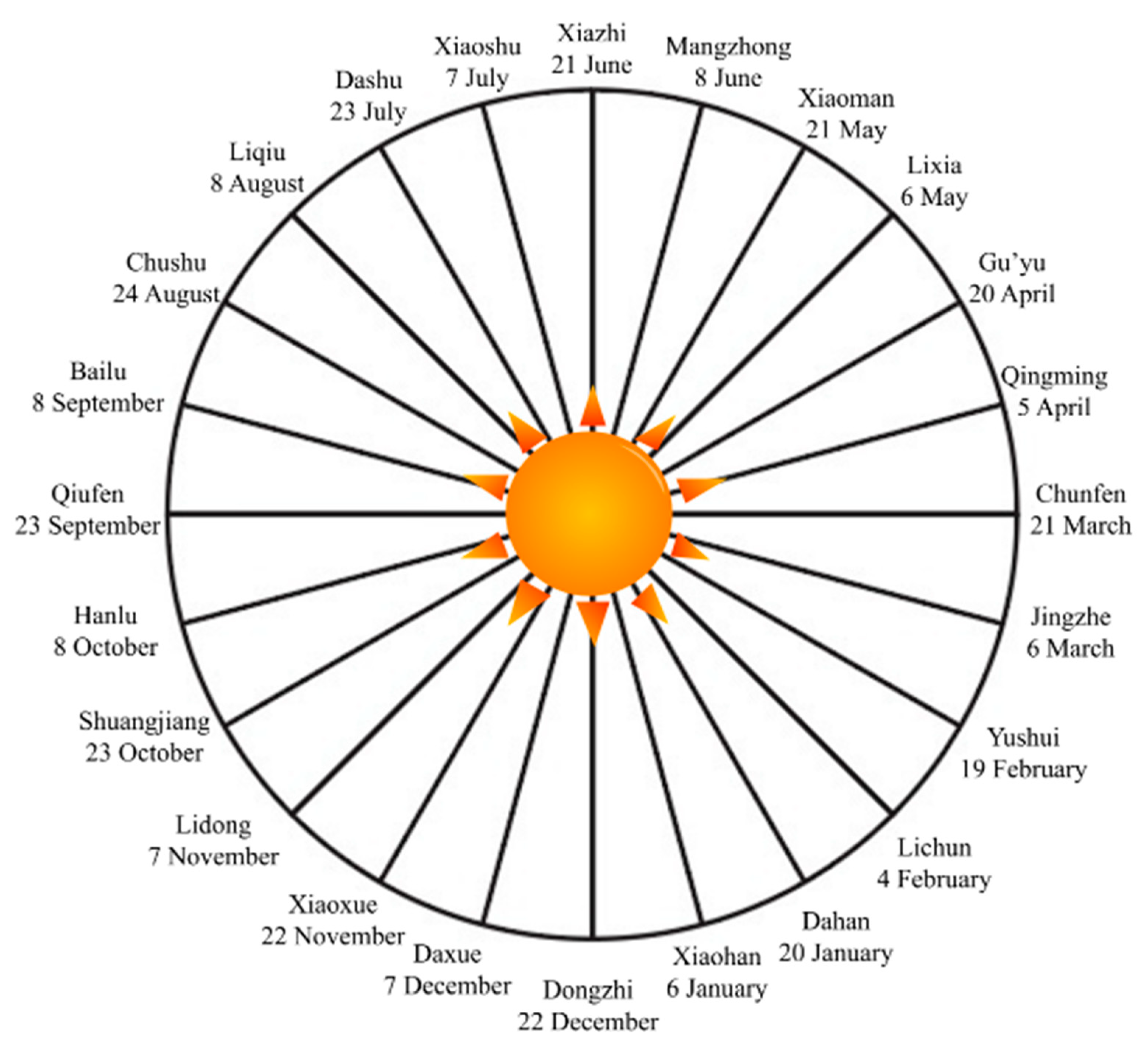
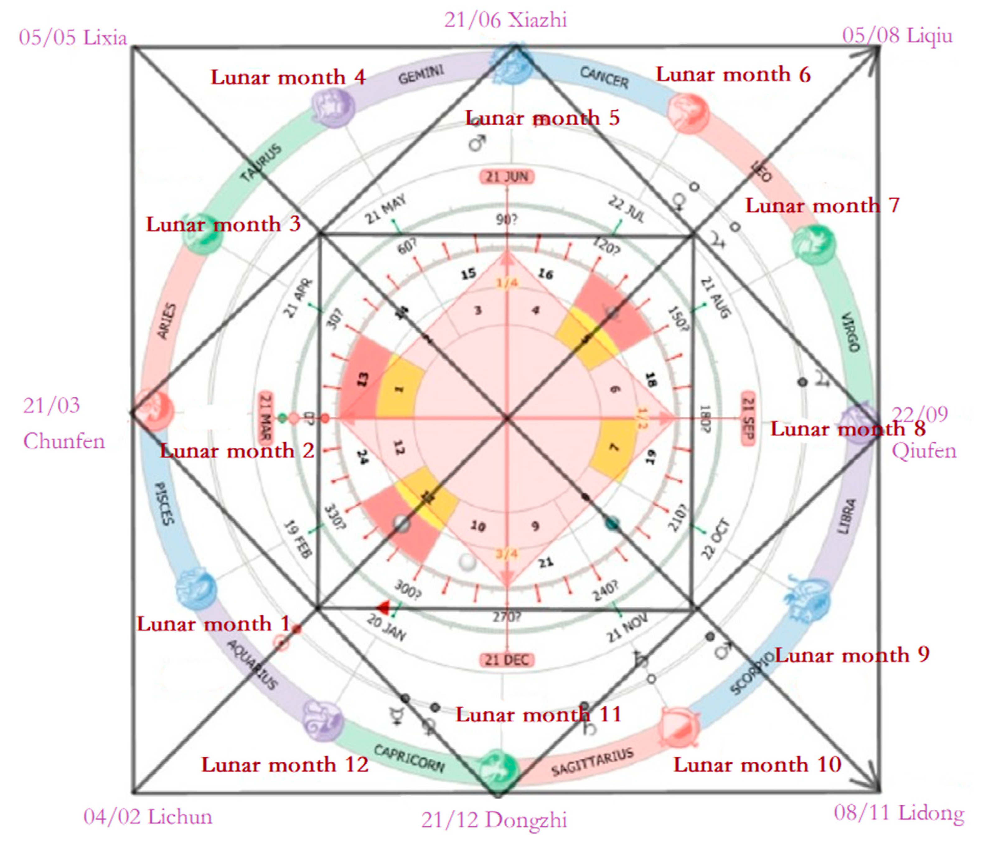
The names of these 24 solar terms are only shown in pinyin and the readers can easily find the explanations online (Table 1). Every solar term has its significant and irreplaceable meaning in the Chinese culture.
What is more, the names of solar terms in the table are ordered according to the Chinese lunar calendar, where Lichun is the first term in a lunar year, Yushui is the second term and Dahan is the last term. However, for convenience, the numbering of solar terms is according to the international solar calendar, in which Xiaohan is the first, happening around 5 January each year while Dongzhi is the last, taking place near 22 December each year. The order above is just for convenience in later mathematical equations.
Definition 3. 
Strong turning point. When n = 20, we call an n-day extreme point a strong turning point P = P ( 20 , t ) .
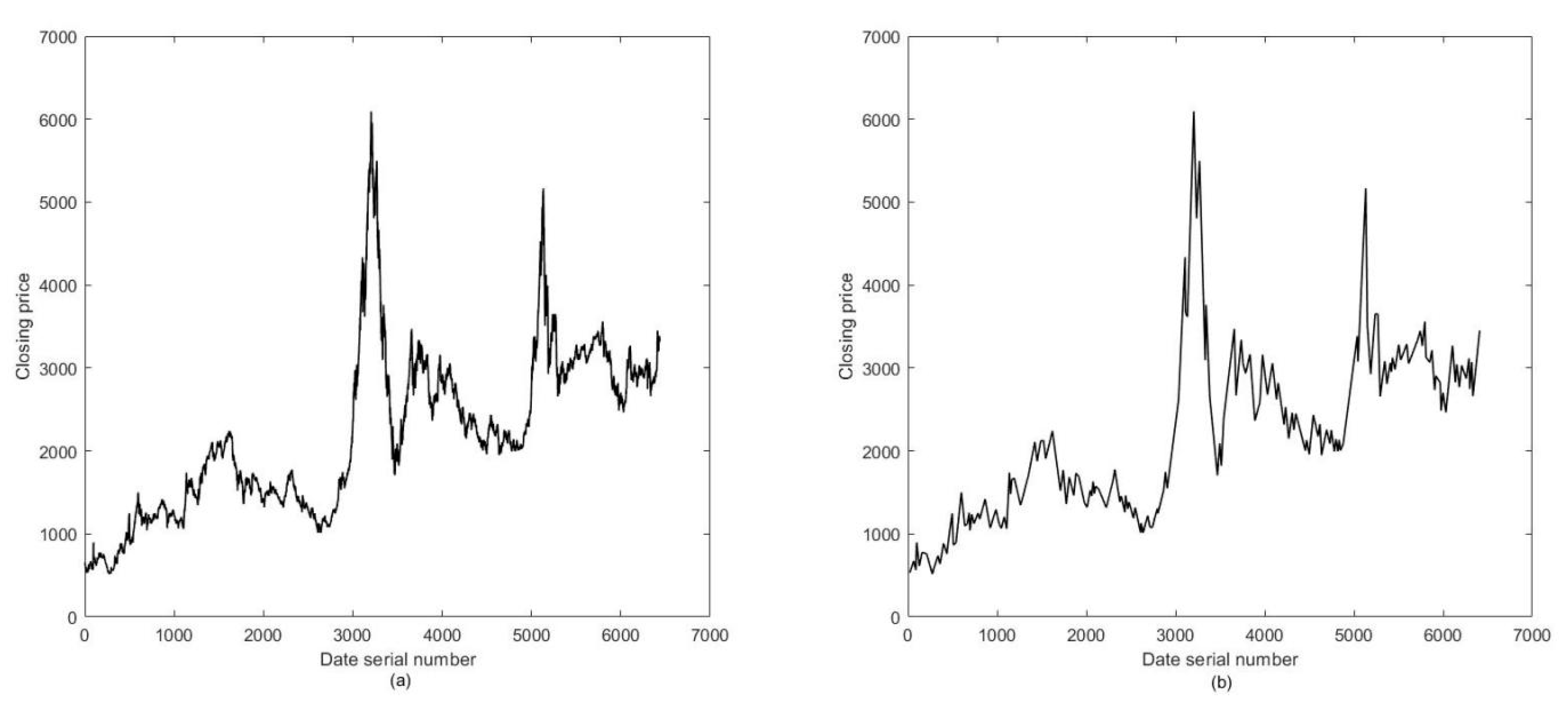
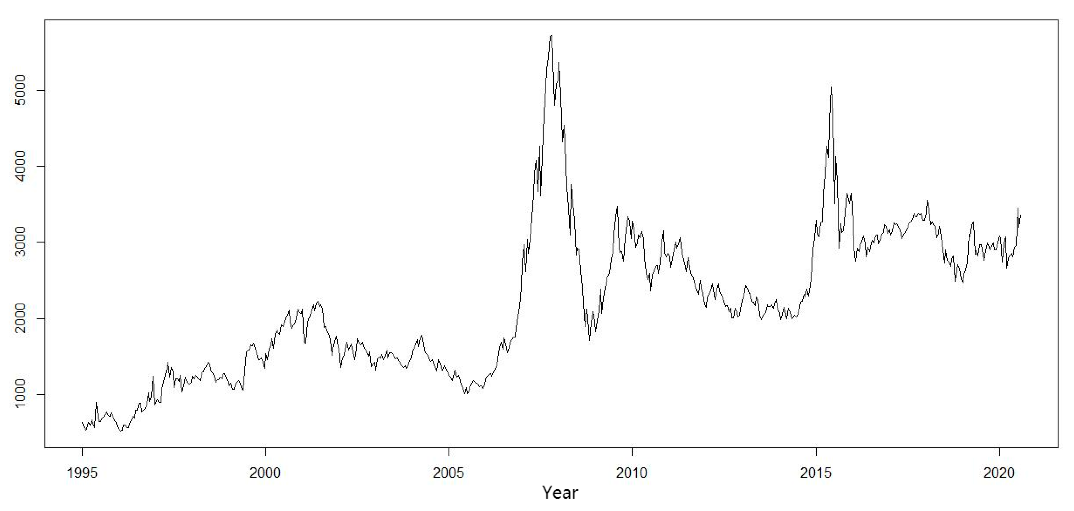
We finally screened out 174 strong turning points. The sequence of strong turning points is { p k 20 } , k = 1, 2, 3…, 174; 6436 daily closing prices of the Shanghai Index were taken from 3 January 1995 to 14 August 2020 (the day this study began); the sequence is x n = x n ( t n ) , n = 1, 2, 3…, 6436, representing the order of market trading days.
We then fitted the daily price based on the interpolation of these 174 strong turning points:
For the adjacent solar points p k 1 20 ,   p k 20 , we set up a linear polynomial:
L k ( x ) = a x + b
L k ( x k 1 ) = p k 1 20
L k ( x k ) = p k 20
Altogether, from all L k ( x k ) , we eventually obtained 6436 interpolated price data (including 174 strong turning points themselves).
We obtained the correlation coefficient ρ = 0.9878
ρ = i = 1 6436 ( h i h m e a n ) ( x i x m e a n ) i = 1 6436 ( h i h m e a n ) 2 i = 1 6436 ( x i x m e a n ) 2
We refined 174 strong turning points to replace 6436 daily price data, which seems to lose a great portion of information; however, it appeared that the 174 strong turning points could still fit the trend of the index in the previous 25 years well. That was because most of the daily price data simply belonged to the link between two adjacent extreme points (may have been strong turning points) and did not have extra information (i.e., every trend had already been presented by two extreme points). Instead, more meaningless price data only bring in more instability, volatility and error that may interfere with the investors’ observations (Figure 3).
That provides a reference for long-term investors: when the price does not reach the extent of a strong turning point (in fact, we often choose n = 10 or 15 for different terms of investment), the index would not have a strong reversal, and the investor can keep holding their stock. When the index goes over or falls below this extent, one would better not expect it to restore soon and it is a time to buy or to sell.
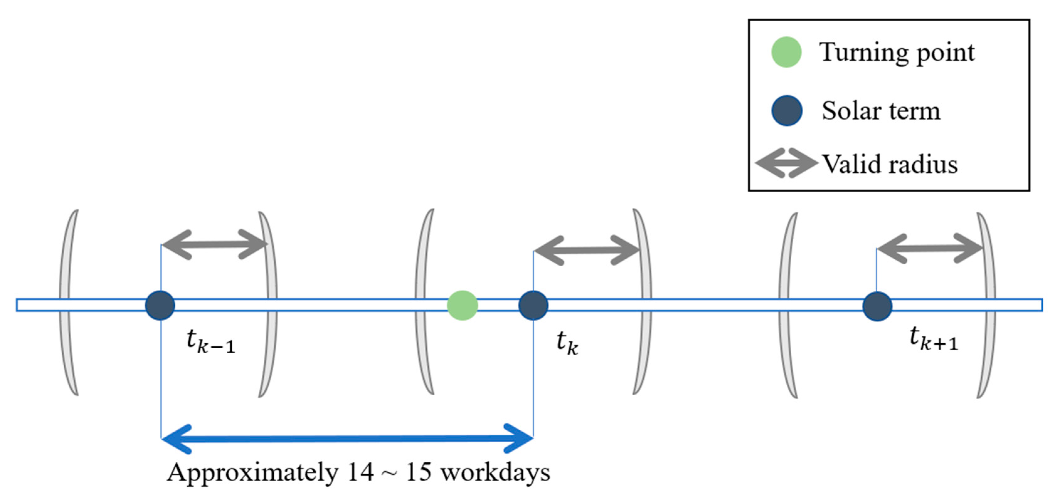
Definition 4.
Valid time radius: m-day valid time radius: when an n-day extreme point is close to the nearest solar term point within m days (before or after), we believe that this n-day extreme point is related to that solar term point and the solar term is valid (Figure 4).

2.2. Valid Extreme Point

TQ refers to the total quantity of n-day extreme points of a stock index while VQ stands for the valid extreme points among those total n-day extreme points. We then used the proportion to estimate the probability of validity (p = proportion = VQ/TQ) which means the probability of p that a solar term causes the reversal of the trend of the stock index.
Here, we showed the proportion of valid turning points and valid 10-day extreme points (Table 2, Table 3, Table 4, Table 5 and Table 6).
The result of the China Second Board Index was similar to the Shanghai index, and that showed the applicability to Chinese stock indices.
In the medium-term and long-term stock investment, the radius conditions of three days and four days were enough to provide a strong reference for investment strategy. The n-day extreme points of different n values often occurred near the solar term point, and investors should pay more attention to the three or four days before and after the solar term. If the price is too high (too low), then we need to be alert. After several verifications with different n, the proportions were similar where the probability was over 80% with the 4-day valid time radius while it only occupies a half of the days between two solar terms (i.e., 4 days before and after occupy 8 days in 15 workdays between adjacent solar terms).
In this way, we supposed that solar terms have an impact on the stock trend and it is like damping, forcing the stock trend to turn or at least hinder its present trend status. With a solar term every 15 days, the stock trend was suggested to have a major change, forming what we saw, ups and downs in serrated fluctuations.
In this section, we verified that a turn or a reversal (i.e., an n-day extreme point, n ≥ 5) always occurred near solar terms.

2.3. Alert Period

In this chapter, we show a practical example of how to react and make actual stock index investment decisions. As we confirmed before, predicting a certain price is almost impossible; thus, we estimated a relative index. Furthermore, we needed to be dynamic, which meant that every movement and change was possible, and we did not set up a goal that it will rise or fall by a specific time; the philosophy is that we judge by the present status, as well as welcome the use of news and other message for assistance.
Based on the efficient markets theory (Eugene Fama, 1970), we were not able to predict the absolute price, but with the statistics above, we were able to provide a relative trend-turning strategy, in which we assess the n value in every daily closing price in the recent days to make dynamic qualitative analysis of the probability of reversal of the coming solar term.
As time goes forward, when it comes to 4 days before a coming solar term, we are in the alert period and when we are 4 days after this solar term, we are out of the alert period.
The period at most lasts for 8 to 9 days but may end earlier if there’s already a significant reversal (or turning point) taking place during the period. As time moves ahead, combine the biggest n value so far in the present alert period and the quantity of the remaining days in the present period; the probability of forecasting whether there is a reversal of the present trend in the period (or turning point) converges to 100%.
Event A t stands for the predictability of the existence of n-day extreme points in one alert period of a solar term. Right now is No.t day of the present alert period.
Event B k stands for no significant reversal of the trend in the first k days in the alert period.
Event C m stands for the biggest n value of the n-day extreme point in the present alert period which we call m for clarity (if the stock index enters an alert period after rising, then we only focus on the low n-day extreme point to be m, and vice versa.)
P.S. A t only means the possibility to make a right judgement or forecast of the trend reversal (i.e., there are n-day extreme points or not) rather than to predict the existence of n-day extreme points. The word “predictability” makes a big difference in the definition. The n value is chosen by investors according to their investment term.
For long-term investment, we suggest it to be over 15, for medium-term investment, it should be around 10, and for short-term investors, n can be around 5.
P ( A t ) = P ( A t | B k ) P ( B k ) = P ( A t | B k ) P ( B k | C m ) P ( C m )
Generally, the alert period of each solar term is no more than 9 days (i.e., 4 days after, 4 days before plus the solar term itself)
Therefore, we have:
lim t 9 P ( A t ) = lim t 9 k 9 [ P ( A t | B k ) P ( B k ) ] = lim t 9 k 9 m + [ P ( A t | B k ) P ( B k | C m ) P ( C m ) ] = 1
In fact, when we use the concept of conditional expectations above, the real probability in the statistics Table 2 and Table 3 is much higher.
The equation provides a dynamic qualitative analysis as we are never sure about the real P(A) under B k and C m which appears not to contradict the efficient markets theory. The stock market contains both relative rules and absolute irregularity at the same time. The best for investor is to use the relative rules as much as possible.
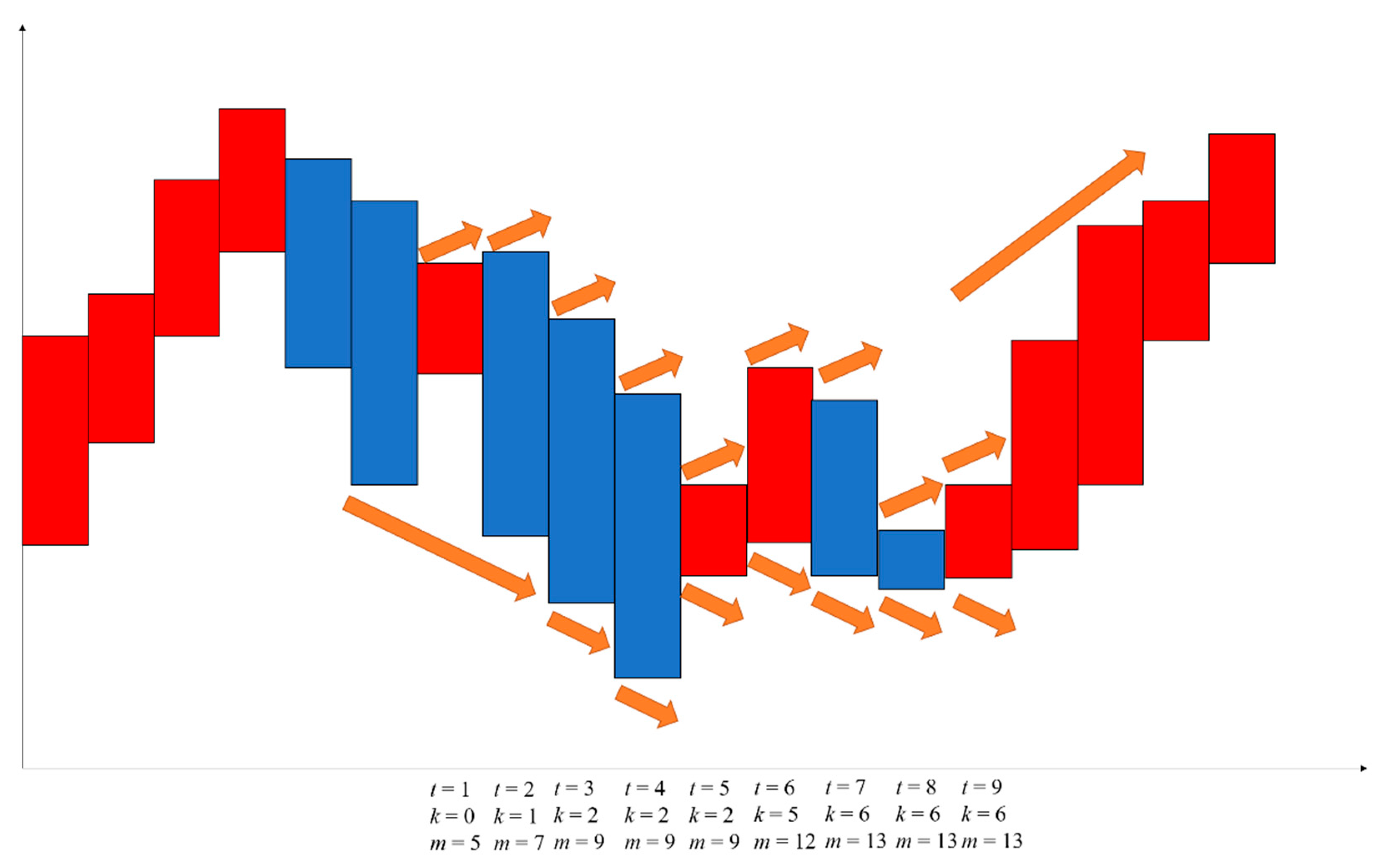
The orange arrows mean the probability to rise or fall and the longer an arrow is, the higher the probability it stands for.
This is a virtual case; we made it to better explain our strategy and vividly show how our method works in real trade (Figure 5 and Figure 6).
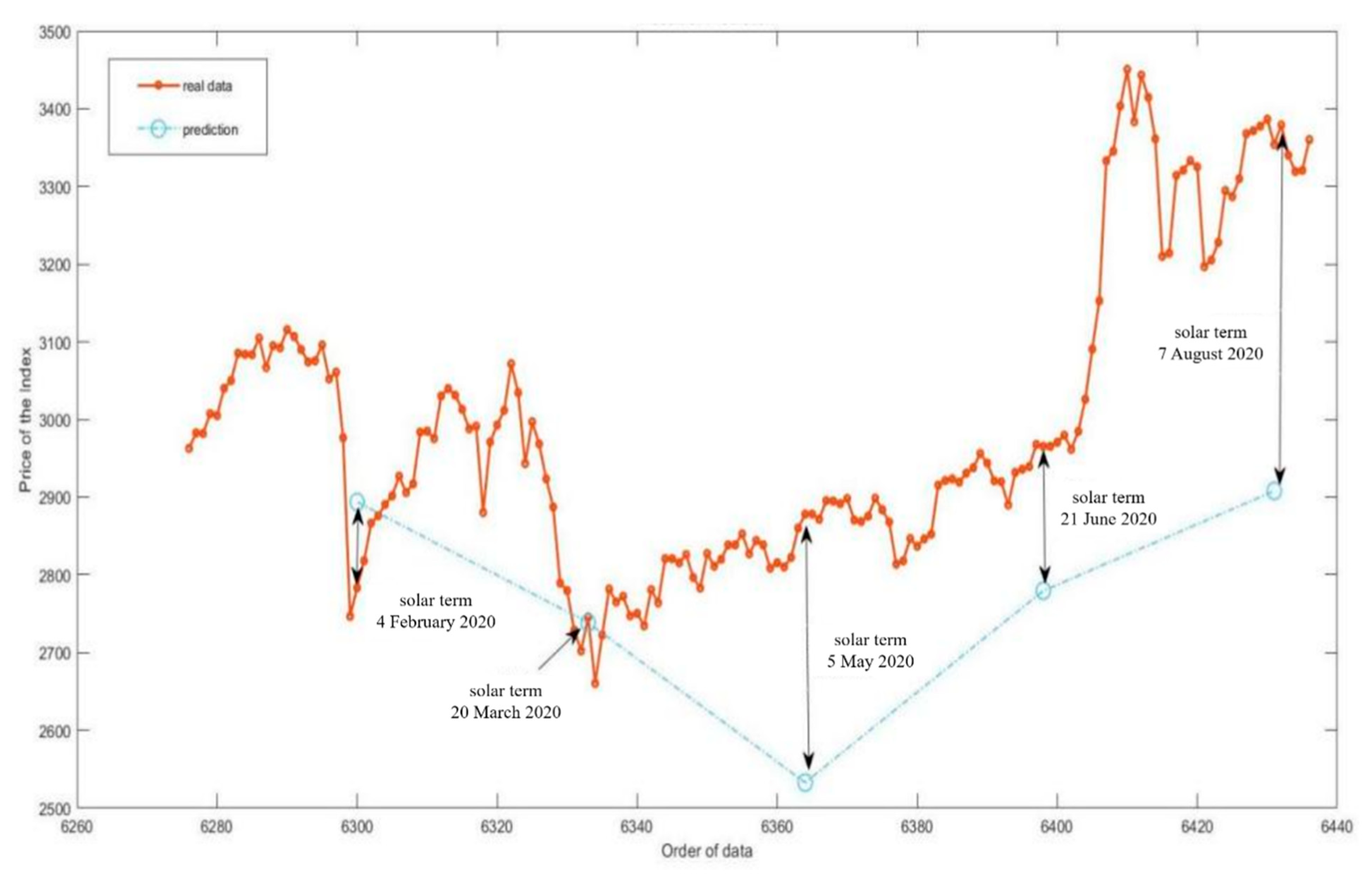
In that case, we found that the actual reversal point (actually, it was a 13-day extreme point) reached the m value of 13 where the price was much lower than that outside the alert period; it also had a very long time to another similar low price.
As the m value becomes bigger and the time is closing to the solar term, we suppose that the possibility of reversal is higher. There may be several signals to show the potential turns and reversal such as t = 5 (goes high after a very low price with a large m value) and t = 9 (the actual turning point). Therefore, the decision should be made dynamically, according to the m and k values in the past. Significant reversals in the alert period are always the real reversal points in stock indices.
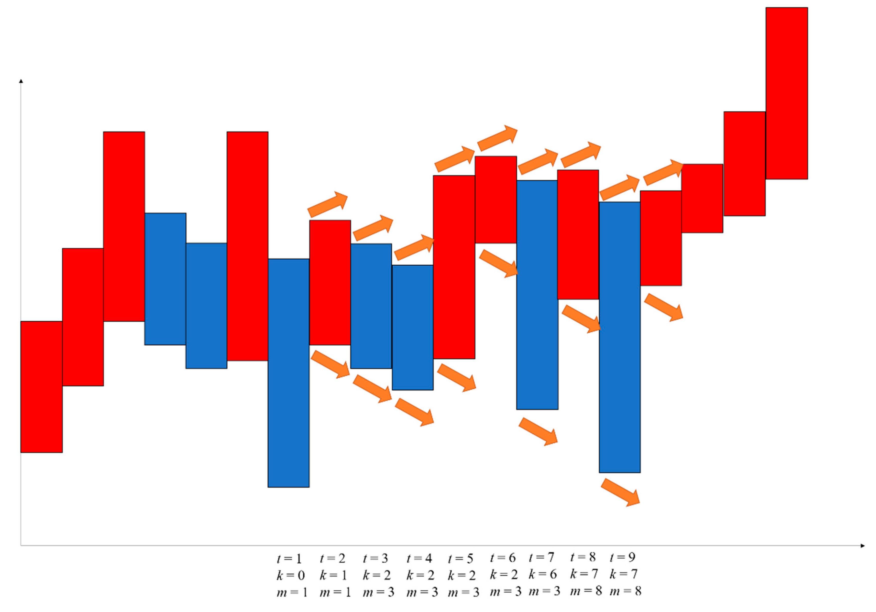
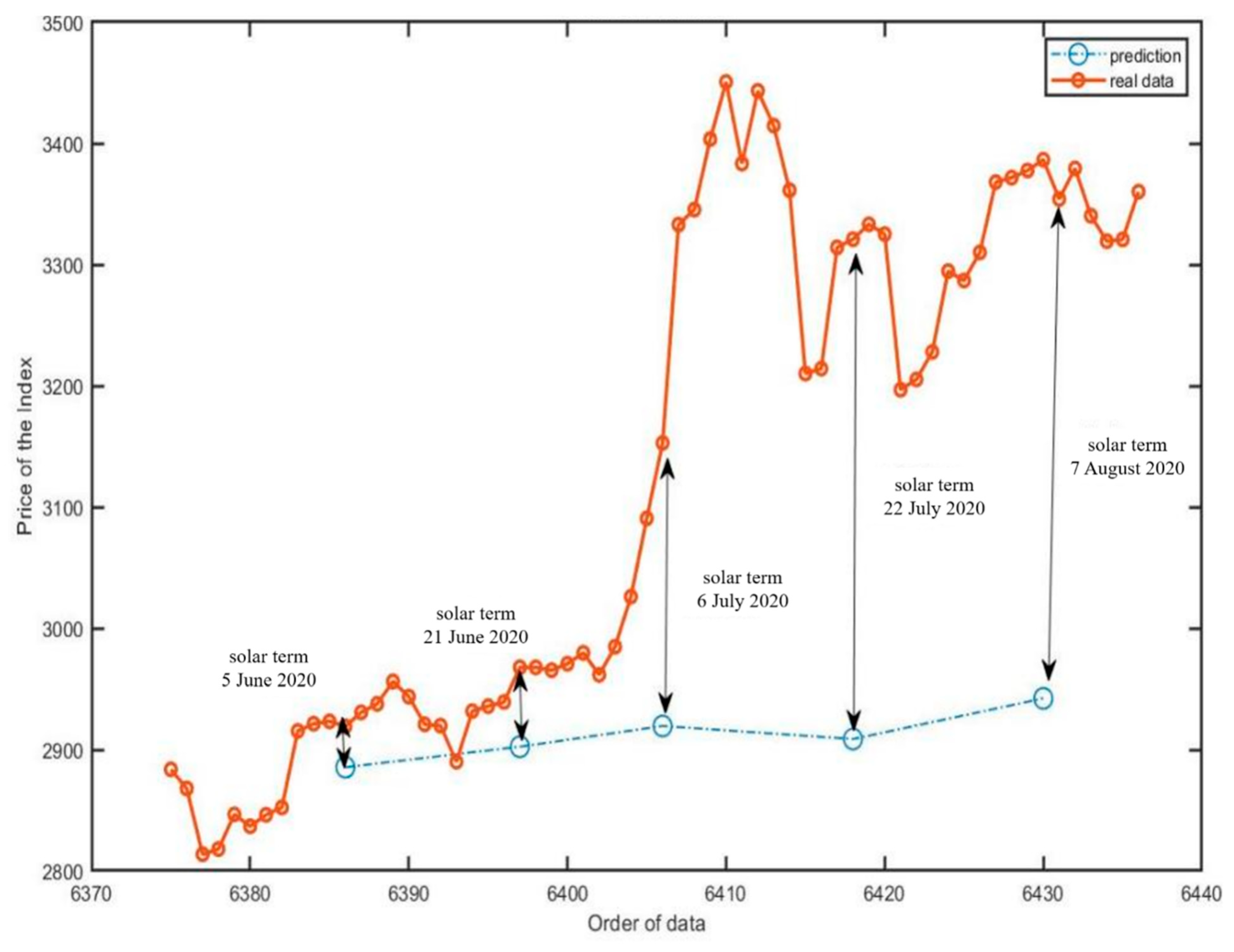
Figure 6 shows a very frequent case where the index does not have a reversal near the solar term; although there are high price and low price when t = 3 or t = 7, it is not low enough compared with a recent extreme point (e.g., the day before t = 1 and 5 days before t = 1). Despite the fact that t = 3 or t = 7 correspond to the two lowest prices in the alert period, there are other lower prices outside the period very close to them, so they do not work.
The case contradicts the common sense, that is, buying on the low and selling on the high; the case proved it only in the alert period, and it is necessary to assess it not according to how many days the stock has been falling in total, but combine the m value it creates with the distance to the solar term.
In other words, while getting closer to the solar term, there is a higher possibility to have a reversal of the trend, but if the biggest n is not so big so far, the probability is always low no matter how close to or far from the solar term it is. The conclusion turns out to be a turbulence but not a reversal or turning point and, in this way, investors can hold their stock at least until the next alert period and the stock index will keep its trend like before the alert period.

2.4. Non-Marketing Day

According to the turnover of the Shanghai Index (actually, it works for all stocks), it is very easy to find out that the turnover in the next day after a weekend or a holiday, in the preparation phase and the first few minutes are very much higher than that in normal marketing days. Thus, we believe that there is still capital flow and transactions allocating for the next marketing day even though they fall on weekends or holidays.
Therefore, we regard each continuous holiday and weekend as one day regardless of whether it contains a solar term. All the statistics described (e.g., the valid time radius) above are applied in this way.

3. Arguments on the Efficient Markets Theory (Hypothesis)

3.1. General Survey of the Efficient Markets Theory (Hypothesis)

The efficient markets theory was first systematically proposed by Eugene Fama (1970) and summarized three forms of the market which are weak form efficiency, semi-strong form efficiency and strong form efficiency. With higher efficiency, the stock price is supposed to be unpredictable and investors do not stably make money through a rule. The efficient markets theory provides us with a fair competing model where everybody is smart and eager to earn money, so there is no exception for one to find out a better way than others.
In a weak form efficient market, stock price cannot be predicted by technological stock analysis (i.e., by applying a mathematical model or numeric analysis to its historical price). In a semi-strong form efficient market, investors only win through inside information and other unfair or illegal methods, and in a strong form efficient market, the stock price is definitely unpredictable at any time.

3.2. Adaptive Market Hypothesis and Imperfection of Efficient-Market Hypothesis

The adaptive market hypothesis (AMH) was proposed to show the predictability and operability of the stock market and its profit [18,19,20]. The AMH also gives us a more realistic perspective compared with the EMH. In fact, the efficient markets theory or the EMH is based on an idealistic model which markets in almost all countries are not yet able to realize; both in developing markets like China and in the developed market of the US, the stock market is only likely to reach the weak level or the semi-strong level which means that there is still a tremendous possibility for regular investors to win [21,22,23], and we accept this possibility, acknowledging that the we still have hope, but we are not going to apply this viewpoint in this paper. In fact, the efficient markets theory has little impact on the time cycle theory and our 24-solar-term method. There is also a study that shows the nonuniversality of the efficient markets theory and found cases to contradict it [24].
First of all, speaking of the efficient markets theory, it always links to historical price and future price (i.e., an absolute numerical value), whereas we focus on the turns and reversal of the trend and the regular changes between the stock and some specific timepoints; we are more likely to conduct a statistics research on the relationship between the stock trend and time which is a relative concept (i.e., when to turn and which timepoint matters more), not an ordinary numeric prediction. Therefore, we talk about neither the historical stock price nor the open financial report, insider information or turnover, we are interested in revealing independent time factors based on the stock market; the time goes forward, and if we handle a rule, we know that something big may happen at a specific timepoint in advance. For example, we know the stock trend probably changes around Chunfen (6), but we have few ideas about the exact time it will take place and what level of price the stock will eventually reach after the effect of Chunfen (6) term, which not only proves that time factors matter but is also consistent with the efficient markets theory.
This was exactly what we wrote in the abstract, “the turns of the stock indices trend were inevitable at specific timepoints while the strength and intensity of the turns were uncertain, affected by various factors by then”, in which we emphasized the certainty of time factors and the remaining uncertainty about the stock.
Secondly, we focused on stock market indices, which were general collections of the stock market, as we knew that a specific stock is surely impossible to predict, but the uncertainty and irregularity are greatly neutralized when it comes to a stock index. The only difference is that if the market efficiency is really weak, our regular analysis would be our second tool, an assistance tool, after the time factor theory (i.e., the time cycle and solar terms theory).

3.3. Why Time Factors Are Superior to the Efficient Markets Theory (Hypothesis)

As we mentioned repeatedly before, the time factor is a four-dimensional factor having an overwhelming impact on our three-dimensional world. Although we can act against the impact it brings, time will forever take the dominant place in the result.
There are several conditions or assumptions in the efficient markets theory about the investors’ mentality, the flow of information and the transactions of money. When all of these conditions are ready, the theory works and the stock becomes unpredictable, but the reality is that the cycle of time and some specific timepoints (i.e., 24 solar terms) always interfere with these conditions, making the efficient markets theory hard to realize in real markets. The tides of moon cause reactions in the human body, and specific timepoints may also lead to emotional instability and irrationality [25,26]. Gann knew the logic and made 286 stock transactions within 25 marketing days from October 1909 and won 264 times under the supervision of The Ticket and Investment Digest [27].
With all the discussion above, we regard the time factor as a natural factor to the human world and prove in this paper that the analysis and forecast on stock trends are practicable.

4. Time Series Analysis of Solar Terms

4.1. Grouping of Solar Terms

Eight of the Chinese 24 solar terms are very prominent, namely, Chunfen (6), Xiazhi (12), Qiufen (18) and Dongzhi (24), which represent the most vigorous timepoints in each season and are the most important four solar terms; the other four are Lichun (3), Lixia (9), Liqiu (15) and Lidong (21). These four represent the beginning of each season and are the second important four solar terms.
To our surprise, the importance of these eight solar terms exactly coincides with the wheel of the cycle theory in Gann theory. In Gann’s wheel, the most important four angles are 90°, 180°, 270° and 360° (0°), and the corresponding timepoints of each year are exactly the four solar terms of Chunfen (6), Xiazhi (12), Qiufen (18) and Dongzhi (24). The second important four angles, 45°, 135°, 225° and 315° exactly correspond to the four solar terms of Lichun (3), Lixia (9), Liqiu (15) and Lidong (21). Regardless of the angle in Gann theory or solar terms, they all point to a common rule, that is, the stock trend is most likely to turn at these eight points. We can summarize the above results as follows: variable or more significant extreme points often occur at the solar term point, and the solar term point usually makes the stock trend turn according to its strength, and the turning strength is large or small.
For convenience, we took the Shanghai Index as an example to present the detailed process of analysis step by step while results of the Second board Index and the Shenzhen Index were directly showed in the following table together with the Shanghai Index using the same approach.
The data we used, as mentioned before, were 6436 daily closing prices from 3 January 1995 to 14 August 2020 of the Shanghai Index (Figure 7); however, we only selected the biggest extreme n-day points near every solar term. In other words, we wanted to select the data of each solar term at the beginning, but since there were bigger n-day points in the 4-day radius, we chose the extreme points to replace every solar term. The total number was not changed.

4.2. Strategy in Analysis

In this chapter, based on the method of random chain [28], analyzing autocorrelation of the price series [29,30,31], we suggested to apply the ARIMA–ARCH time series model to fit and forecast the index as time series analysis is a modern tool for predicting. Time series models, meanwhile, can introduce long-term correlation cases and their volatility dealing with price, production, population growth, etc.
In general, the autocorrelation (hereinafter referred to simply as the “correlation”) of a stock index is long-term; thus, it may involve a great deal of data for a regular time series analysis, making the model extremely complicated and inaccurate.
Besides, the traditional time series fitting is based on high-frequency data (i.e., daily closing prices) on continuous marketing days. However, most of the high-frequency data are meaningless as they are only the trend connection between two turning points and have no special significance. Those high-frequency data contribute nothing but add more error, volatility and turbulence that mislead investors into believing them to be a turn.
Considering the intervals are almost equal between two solar terms, it is suitable to use the extreme points around each solar term as items in the time series. By doing this, we actually extract representatives of every trend and magnify the period in the analysis (i.e., two solar terms cover around 15 days; that is 15 times more than when simply applying two daily prices).
Throughout this paper, we only focused on the forecast of the index trend, not the price.
For the stationary time series after the difference, we used the ARIMA model to fit [32]. ARIMA is the autoregressive integrated moving average model denoted ARIMA(p,d,q).
{ Φ ( B ) = d x t = Θ ( B ) ε t E ( ε t ) = 0 ,   V a r ( ε t ) = σ ε 2 ,   E ( ε t ε s ) = 0 ,   s t E ( x s ε t ) = 0 ,   s < t
where d = ( 1 B ) d ;   Φ ( B ) = 1 φ 1 B φ p B p is the autoregressive coefficient polynomial of the ARIMA model; Θ ( B ) = 1 θ 1 B θ q B q is the moving average coefficient polynomial of the ARIMA model.
The sequence after the d-order difference is
d x t = i = 0 d ( 1 ) i C d i x t i = Θ ( B ) Φ ( B ) ε t
where { ε t } is the white noise sequence with the zero mean.
For the residual sequence with heteroscedasticity, we have the autoregressive conditional heteroskedastic model ARCH(q) [33]. By using an ARCH(q) model, we can characterize the conditional variance changing with time.
The structure of the ARCH(q) model is as follows: assuming that the historical data are known, the sequence of the zero mean residuals has heteroscedasticity.
E ( ε t ) = 0 ,   V a r ( ε t | ε t 1 , ε t 2 ) = h t
h t = λ 0 + i = 1 q λ i ε t i 2
The ARCH(q) model requires existence of non-negative variance and unconditional variance.
V a r ( ε t | ε t 1 , ε t 2 ) = λ 0 + i = 1 q λ i ε t i 2 0
where λ 1 , λ 2 , λ q 0 ,
V a r ( ε t ) = σ 2
where 0 λ i < 1 , λ 1 + λ 2 + + λ q < 1 .
The 24 solar terms were divided into four groups: the all-terms group (all 24 solar terms), four-terms group A (Lichun (3), Lixia (9), Liqiu (15) and Lidong (21)), four-terms group B (Chunfen (6), Xiazhi (12), Qiufen (18) and Dongzhi (24)) and the eight solar terms group (altogether, there were eight solar terms). The historical data were divided into the experimental group and the test group (the last five solar terms).

4.3. Time Series Analysis of the All-Terms Group

According to Cramer’s decomposition theorem (Cramer, 1961), nonstationary sequence can be decomposed as follows:
x t = j = 0 d β j t j + ψ ( B ) α t
where { α t } is the white noise sequence with the zero mean.
We found that the stock data had an upward trend, so it was necessary to make a first-order difference to meet the stationarity of the series [34].
x t = x t x t 1
In this database, we had 615 solar terms through about 25 years, thus, x t stood for the price of each solar term (Figure 8).
In fact, we used the biggest n-day extreme price with a 4-day radius to represent the price of one solar term, and we did not distinguish them in the following part, calling all of them the price of a solar term.
The daily return of the Shanghai stock index fluctuated around the average value of 0, and the fluctuation was different in different periods. It fluctuated sharply in 2007–2008 and in 2015 while it was relatively stable in other periods (Table 7).
The p-value of the Jarque normality test was close to zero, which showed that the stock data did not follow the normal distribution. The p-value of the ADF test was much lower than 0.05. We thought the stability was satisfactory then.
Null hypothesis: H 0 : ρ 0 while H 1 : ρ < 0 .
The ADF test statistics value was calculated as follows:
τ = ρ ^ S ( ρ ^ )
where S ( ρ ^ ) is the standard error of ρ ^ .
If it is stationary, the result is ρ   < 0.
Due to its obvious cluster of volatility, experience and common sense, we generally think that stock data are heteroscedastic, so we need to carry out next a heteroscedasticity test. As shown in the figure, the square sequence of the stock data showed significant autocorrelation (Table 8 and Figure 9).
Since the residual may be autocorrelated, we used the autoregressive model to fit the sequence of the square residual.
ε t 2 = ω + j = 1 q λ j ε t j 2 + e t
Null hypothesis: H 0 :   all   λ i = 0 while H 1 :   at   least   one   λ = 0
LM ( q ) ~ χ 2 ( q 1 )
We then looked at the sequence after the one-order difference. We conducted the LM test: the p-value of the ARCH–LM test was 2.2 × 10⁻¹⁶, so we rejected the original hypothesis and accepted there was the ARCH effect. In conclusion, the return sequence of the Shanghai stock index (i.e., the price sequence after the first-order difference) had the ARCH effect (Table 9, Figure 10 and Figure 11).
Firstly, we established an ARIMA model [35] for the mean value of the series of the all solar terms group of the Shanghai stock index and selected the last five solar terms to examine the forecast. After a repeated comparison, we chose ARIMA(36, 1, 12) and in fact, in some mathematical forecasts, the parameters were often large [36] as our data were very complicated and was never auto-correlated only in the short term [37,38,39,40,41].
We found that the ARCH(2) model made a good fit for the residual of several periods with obvious fluctuation (Figure 12). The Ljung–Box test showed that the p-value was much bigger than 0.05, that is, the residual and the square of the residual after the process of the ARCH model were white noise sequences, which indicated that the original sequence information was fully extracted by the ARCH(2) model.
Although GARCH(1,1) is also used in many economic analyses, ARCH(2) still did a good job in reflecting volatility in the index as the volatility we forecast was just a quality analysis and we only needed to know the comparative value (i.e., when it is bigger, when it is lower) rather than a certain degree of volatility. GARCH(1,1) is for long-term volatility fitting, but the way we established our model (i.e., using extreme points near solar terms) already made the term long enough, so the coefficient of GARCH(1,1) resulted in an insignificant level.
Finally, we obtained the following ARIMA(36, 1, 12)–ARCH(2) model for the all-terms group (Table 10):
Mean model:
x n = i = 1 36 a i · x n i + j = 1 12 b j · ε n j + ε n
Variance model:
ε n = h n e n ,   e n   is   an   i . i . d .   random   variable   with   X ~ N ( 0 , 1 )
h n = 7071 + 0.5220 ε n 1 2 + 0.2657 ε n 2 2
According to the model, the forecast of five periods in the future is as follows (Table 11 and Figure 13).
Now we make analysis of other groups (Table 12 and Table 13)
We would like to make an explanation here since the figure may be a bit small. The orange line is the real trend that links orange points which are the daily closing prices of the index while the blue line links several blue points which are the forecast prices on solar terms. Every forecast price on each solar term was matched to the real price, showing the gap in the price and the shape of the trend.
We found that there was a certain difference in forecasting the future stock price at the future solar terms by using the historical solar terms; however, the forecast of the trend was very accurate, and the trend in the future period was consistent with the real trend.
In that case, we were informed what the next trend would be like so that, combined with the methods in the chapters before, we would have a better handling of our investment. This was a quality analysis as we were never able to calculate the profit, costs, risks, etc. in the future; otherwise it would contradict the efficient markets theory.
The time series analysis in this paper was for trend reversal, so we paid more attention to the turning of the trend at solar terms rather than to the absolute price.

4.4. Time Series Analysis of the Eight-Terms Group

As mentioned before, the time series plot of the eight important solar terms each year also described the historical trend of the stock well.
In the ACF, PACF test and the ACF, PACF test of residuals, the results of the eight solar terms group highly coincided with those of the all solar terms group, so we still used the ARIMA(36, 1, 12)–ARCH(2) model to process the data in the same way. Here, the model parameters and formulas were omitted, and the results were as follows (Table 14, Table 15 and Table 16 and Figure 14):
We could see that, like in the all-terms group, the time series analysis had some errors in forecasting, but it could better forecast the trend of stocks in the future. In fact, there were two trends from the first period to the second period in the future, falling one by one. However, the stock finally bottomed out on 22 March. The forecast trend of the second period to the third period in the future was wrong, showing a certain delay. However, by the fourth period in the future, the forecast value increased sharply, showing the correction of the previous error. When the fifth period in the future was reached, the trend forecast coincided with the actual trend.

4.5. Time Series Analysis of the Four-Terms Group

After many attempts, the forecast was still not good, indicating an obvious deviation with the real data of the test group. Therefore, we believe that it would be better to forecast using all solar terms or eight solar terms. The data is lost to a great extent if we use very few solar terms to forecast. Thus, we do not recommend conducting a time series analysis with few solar terms.

5. Conclusions

Individual stocks were confirmed to be unpredictable and stochastic according to the EMH and AMH. Even though the efficiency of the stock market around the world did not reach an idealistic level, generally speaking, it was still very hard and ineffective for investors to forecast a certain stock. Analyzing the three major indices of the China’s stock market was a good tool to cover all stock categories in the market while making the study more practicable and reasonable.
However, stock indices proved to be rather predictable to some extent. Therefore, according to the study, investors can invest in ETFs that belong to the indices as an ETF is completely coincidental with the index it belongs to. Furthermore, ETFs provide investors with a variety of options of risk and profit. The Shanghai ETF is smooth whereas the Second Board 50 Fund fluctuates a lot. Investors are able to get a high profit from individual stocks as well through implementing the results of this study.
The correlation between the turning points of indices and the Chinese 24 solar terms was positive ( ρ = 0.9878).
Turning points always occur near solar terms. Through testing n-day extreme points with a different n value, the sharp turns of the trend often happened near the solar terms, and if we choose 4 days as the valid time radius, the probability is about 80%. Investors should be alert for four days before and four days after a solar term. If the price is too high (low), it is more likely to be affected by the coming solar term, and the higher (lower) the price is, the more instability the trend then would have.
However, solar terms are not always strong turning points, but they might cause weaker turning points. In other words, solar terms might not cause a sharp reversal of the stock trend; strong turning points were just some exceptions. Usually, the turning points were not that strong but sufficient for medium-term and short-term investors.
The alert period provided investors with a good strategy for short-term and medium-term trading. When judging the upcoming reversal, it should be dynamic. According to the practical examples in the alert period, investors should also notice significant signals such as the present n-day extreme points combined with the distance to the solar term. By understanding the alert period carefully, investors would have a positive profit in their future investment.
The 24 solar terms in each year and their links accurately fitted the trend of the stock in that year. Using 24 price datapoints instead of nearly 250 daily datapoints of the whole year could make the daily data of high frequency more concise and easier to process. With 250 high-frequency daily datapoints, there is strong volatility, which leads to the obvious heteroscedasticity of the data and increases the complexity of data analysis. The use of 24 solar terms instead of annual data also greatly reduces this unstable and irregular fluctuation. This also coincides with Gann theory.
The forecast of future trends in the all-terms group and the eight-terms group was precise, but there remained a gap with the absolute price. We were only able to forecast the timepoints and the turning points; as for the absolute price, we hardly made it. This is because the stock market involves a great deal of instability and is extremely complicated. Besides, through the failure of the four-terms group, we found that we should not choose too few solar terms and that every solar term is equal, having its own meaning and function, and all of them represent trends of certain periods.

6. Philosophy and Deeper Discussion

This chapter is an extension of Section 1.4; we make a brief review and discuss something valuable that we may be able to apply in other studies.
The fact is that the turning of the stock trend has rules to follow, which is the inevitable result at specific timepoints, while the strength and intensity of the turning is uncertain, affected by various factors at that time. The stock market contains both certainty and uncertainty at the same time, where natural instincts play a role as the inner factor while the environment—as an outer factor. Like the EMH and the AMH, they mainly focus on the outer factor, in other words, they prefer to look at those changeable things. However, as we were inspired by Gann, Elliott and the Chinese 24 solar terms, we would rather look for those that do not change, and that is the key to have a better understanding and cognition of our real world, of course, including the stock market.
For this reason, it is the higher dimensional time factor and time cycle that produce an overwhelming impact on the stock market, so it reminds us of taking into account the importance of time when conducting such a study. That is why Gann summarized a tremendous amount of time periods to inform the possible reversal in the capital market while the ancient Chinese figured out 24 divisions of a year as 24 solar terms which all solely point to time.
In addition, the ancient Chinese elaborated a complex system, and there are actually many other divisions of time, years, months, etc. in the Chinese culture. For example, the ten heavenly stems and the twelve earthly branches decide what a year would be like, and that is a 60-year cycle as there are 60 different combinations of one out of the ten heavenly stems with one out of the twelve earthly branches. By the way, one combination is called Gengzi, which is supposed to be the year of disasters and conflicts; the latest Gengzi year was 2020.
We encourage other researchers to explore and apply our approach to other fields to see whether there is a rule to follow based on time factors. We will also demonstrate our method to other foreign stock markets. We also suggest that researchers read more ancient works, books and references related to time divisions and time factors, hoping our study will open a brand-new door in financial analysis.

Author Contributions

Conceptualization, T.Z.; methodology, T.Z. and X.L.; software, X.L.; investigation, T.Z. and X.L.; data curation, X.L.; writing, T.Z. and X.L.; supervision, P.W. All authors have read and agreed to the published version of the manuscript.

Funding

This research received no external funding.

Institutional Review Board Statement

Not applicable.

Informed Consent Statement

Not applicable.

Data Availability Statement

All the data are free and available to download from https://money.163.com (accessed on 28 February 2021).

Conflicts of Interest

The authors declare no conflict of interest.

References

  1. Colin-Jaeger, N.; Delcey, T. When efficient market hypothesis meets Hayek on information: Beyond a methodological reading. J. Econ. Methodol. 2020, 27, 97–116. [Google Scholar] [CrossRef] [Green Version]
  2. Mehdi, Z.; Samad, G. A hybrid approach of adaptive wavelet transform, long short-term memory and ARIMA-GARCH family models for the stock index prediction. Expert Syst. Appl. 2021, 182. [Google Scholar] [CrossRef]
  3. Kuhe, D.A. The Dynamic Relationship between Crude Oil Prices and Stock Market Price Volatility in Nigeria: A Cointegrated VAR-GARCH Model. Curr. J. Appl. Sci. Technol. 2019, 1–12. [Google Scholar] [CrossRef]
  4. Gan, X. Study on the Correlation between the Changes of Four Seasons and Solar Terms and the Dynamics of Some Physiological Indexes of Human Body. Master’s Thesis, Beijing University of Chinese Medicine, Beijing, China, 2013. Available online: https://kns.cnki.net/kcms/detail/detail.aspx?FileName=1013205433.nh&DbName=CMFD2013 (accessed on 28 February 2021).
  5. Gong, G. Stock Market and 24 Solar Terms. Bus. China 2008, 5, 124. Available online: https://kns.cnki.net/kcms/detail/detail.aspx?FileName=JSGZ200805059&DbName=CJFQ2008 (accessed on 28 February 2021).
  6. Hede, C. 24 Solar Terms and the Turning Point of Stock Market. Stock. Mark. Trend Anal. Wkly. 2008, 52, 24. Available online: https://kns.cnki.net/kcms/detail/detail.aspx?FileName=FSDT200852011&DbName=CJFQ2008 (accessed on 28 February 2021).
  7. Wang, W. A Study on the Solar Term Effects of Stock Market. Master’s Thesis, Southeast University, Nanjing, China, 2017. Available online: https://kns.cnki.net/kcms/detail/detail.aspx?FileName=1018003229.nh&DbName=CMFD2018 (accessed on 28 February 2021).
  8. Liu, D. Research on the Core Thoughts of Gann’s Investment Theory and Applications. Master’s Thesis, Dongbei University of Finance and Economics, Dalian, China, 2010. Available online: https://kns.cnki.net/kcms/detail/detail.aspx?FileName=1011065695.nh&DbName=CMFD2012 (accessed on 28 February 2021).
  9. Gann, W.D. The W. D. Gann Master Commodity Course; Snowball Publishing: Dallas, TX, USA, 2009. [Google Scholar]
  10. Gann, W.D. 45 Years in Wall Street; Wilder Publications: Saint Paul, MN, USA, 2014. [Google Scholar]
  11. Morena, C. Unlocking W. D. Gann’s Methods; Amazon Independently Published: Bellevue, WA, USA, 2020. [Google Scholar]
  12. Hyerczyk, J.A. Pattern, Price and Time; Wiley: Hoboken, NJ, USA, 2009. [Google Scholar]
  13. McMillan, D.G. Non-linear predictability of UK stock market returns. Oxf. Bull. Econ. Stat. 2003, 65, 557–573. [Google Scholar] [CrossRef]
  14. Ali, S.R.M.; Ahmed, S.; Hasan, M.N.; Östermark, R. Predictability of Extreme Returns in the Turkish Stock Market. Emerg. Mark. Financ. Trade 2021, 57, 482–494. [Google Scholar] [CrossRef]
  15. Paul, B. McGuinness, Turn-of the-month’ return effects for small cap Hong Kong stocks. Appl. Econ. Lett. 2006, 13, 891–898. [Google Scholar] [CrossRef]
  16. Yadav, S.P. Calendar Anomaly in Indian Stock Market with Respect to Empirical Study of Quarter of the Year Effect, Month of the Year Effect, Day of the Week Effect on NIFTY for the Years Jan. Vishwakarma Bus. Rev. 2013, 3, 76–85. Available online: https://schlr.cnki.net/zn/Detail/index/SFJG_01/SFJGC115080C8D7892EDA0B7A4ED71F129CD (accessed on 31 March 2021).
  17. Urquhart, A.; McGroarty, F. Calendar effects, market conditions and the Adaptive Market Hypothesis: Evidence from long-run U.S. data. Int. Rev. Financ. Anal. 2014, 35, 154–166. [Google Scholar] [CrossRef]
  18. Tripathi, A.; Vipul, V.; Dixit, A. Adaptive market hypothesis and investor sentiments: Global evidence. Manag. Financ. 2020, 46, 1407–1436. [Google Scholar] [CrossRef]
  19. Xiong, X.; Meng, Y.; Li, X.; Shen, D. An empirical analysis of the Adaptive Market Hypothesis with calendar effects: Evidence from China. Financ. Res. Lett. 2019, 31. [Google Scholar] [CrossRef]
  20. Dhankar, R.S.; Shankar, D. Relevance and evolution of adaptive markets hypothesis: A review. J. Indian Bus. Res. 2016, 8, 166–179. [Google Scholar] [CrossRef]
  21. Abubakar, M. A Survey of Literature on Theory and Empirics of Efficient Market Hypothesis. Asian J. Econ. Bus. Account. 2017, 1–8. [Google Scholar] [CrossRef]
  22. Bhattarai, K.; Margariti, V. An Empirical Test of the Theory of Efficient Markets of Stock Prices. Financ. Mark. 2018, 3. [Google Scholar] [CrossRef] [Green Version]
  23. Zhang, H.; Wei, J.; Huang, J. Scaling and predictability in stock markets: A comparative study. PLoS ONE 2017, 9. [Google Scholar] [CrossRef] [PubMed]
  24. Ansari, M.; Jafari, H. The Effect of Market Anomalies on the Inefficiency of Stock Returns. Am. J. Theor. Appl. Bus. 2020, 6, 23–27. [Google Scholar] [CrossRef]
  25. Cohen-Charash, Y.; Scherbaum, C.A.; Kammeyer-Mueller, J.D.; Staw, B.M. Mood and the market: Can press reports of investors’ mood predict stock prices? PLoS ONE 2017, 8. [Google Scholar] [CrossRef] [PubMed] [Green Version]
  26. Wang, Y.; Lin, C.; Lin, J. Does weather impact the stock market? Empirical evidence in Taiwan. Qual. Quant. 2012, 46, 695–703. [Google Scholar] [CrossRef]
  27. Billy, J. The W.D. Gann Technical Review; Wu, J., Ed.; Shanxi People’s Publishing House: Taiyuan, China, 2015. [Google Scholar]
  28. Working, H. Note on the Correlation of First Differences of Averages in a Random Chain. Econometrica 1960, 28, 916–918. [Google Scholar] [CrossRef]
  29. Krämer, W.; Runde, R. Testing for autocorrelation among common stock returns. Stat. Pap. 1991, 32, 311–320. [Google Scholar] [CrossRef]
  30. Lim, K.; Luo, W.; Kim, J.H. Are US stock index returns predictable? Appl. Econ. 2013, 45, 953–962. [Google Scholar] [CrossRef]
  31. Booth, G.G.; Koutmos, G. Interaction of volatility and autocorrelation in foreign stock returns. Appl. Econ. Lett. 1998, 5, 715–717. [Google Scholar] [CrossRef]
  32. Wang, Y. Applied Time Series Analysis, 5th ed.; China Renmin University Press: Beijing, China, 2016. [Google Scholar]
  33. Tsay, R.S. Analysis of Financial Time Series, Wiley-Interscience, 2nd ed.; Wiley: Hoboken, NJ, USA, 2012. [Google Scholar]
  34. Chang, Y.; Feng, Y.; Cao, X. Analysis and Prediction of Stock Price Based on Non Linear Time Series Model. Math. Pract. Theory 2018, 48, 21–26. Available online: https://kns.cnki.net/kcms/detail/detail.aspx?FileName=SSJS201822003&DbName=DKFX2018 (accessed on 31 March 2021).
  35. Feng, P.; Cao, X. An Empirical Study on the Stock Price Analysis and Prediction Based on ARMA Model. Math. Pract. Theory 2011, 22, 84–90. Available online: https://kns.cnki.net/kcms/detail/detail.aspx?FileName=SSJS201122012&DbName=CJFQ2011 (accessed on 30 May 2021).
  36. Liu, S.; Zhu, Y.; Zhang, K.; Gao, J. Short-term wind power forecasting based on error correction arma-garch model. Acta Energy Sol. Sin. 2020, 41, 268–275. Available online: https://kns.cnki.net/kcms/detail/detail.aspx?FileName=TYLX202010036&DbName=DKFX2020 (accessed on 31 March 2021).
  37. Gulen, S.; Popescu, C.; Sari, M. A New Approach for the Black–Scholes Model with Linear and Nonlinear Volatilities. Mathematics 2019, 7, 760. [Google Scholar] [CrossRef] [Green Version]
  38. Albulescu, C.T.; Tiwari, A.K.; Kyophilavong, P. Nonlinearities and Chaos: A New Analysis of CEE Stock Markets. Mathematics 2021, 9, 707. [Google Scholar] [CrossRef]
  39. Caraiani, P. Testing for nonlinearity and chaos in economic time series with noise titration. Econ. Lett. 2013, 120, 192–194. [Google Scholar] [CrossRef]
  40. Fama, E.F. Efficient capital markets: A review of the theory and empirical work. J. Financ. 1970, 25, 383–417. [Google Scholar] [CrossRef]
  41. Wang, P.; Moore, T. Stock market integration for the transition economies: Time-varying conditional correlation approach. Manch. Sch. 2008, 76, 116–133. [Google Scholar] [CrossRef] [Green Version]
Figure 1. Time that each solar term takes place annually.
Mathematics 09 01713 g001
Figure 2. Twenty-four solar terms, 12 earthly branches in China corresponding to the Western calendar and constellation (From Sina Weibo, author: KENUT).
Mathematics 09 01713 g002
Figure 3. (a) Original index data by turning points of the Shanghai Index. (b) Fitted data by turning points of the Shanghai Index.
Mathematics 09 01713 g003
Figure 4. Valid time radius.
Mathematics 09 01713 g004
Figure 5. Practical example of the alert period (stock falling case).
Mathematics 09 01713 g005
Figure 6. Practical example of an alert period (turbulence case between two ascending trends).
Mathematics 09 01713 g006
Figure 7. Time series plot of the Shanghai stock index in 1995–2020.
Mathematics 09 01713 g007
Figure 8. Result after the first-order difference of the Shanghai Index (daily revenue).
Mathematics 09 01713 g008
Figure 9. Lag (a) ACF plot after the first-order difference of the Shanghai Index. Lag (b) PACF plot after the first-order difference of the Shanghai Index.
Mathematics 09 01713 g009
Figure 10. Lag (c) Squared ACF plot after the first-order difference of the Shanghai Index. Lag (d) Squared PACF plot after the first-order difference of the Shanghai Index.
Mathematics 09 01713 g010
Figure 11. ARCH(2) model’s residual of the Shanghai Index’s daily revenue.
Mathematics 09 01713 g011
Figure 12. Fitted volatility of the ARCH(2) model’s residual of the Shanghai Index’s daily revenue.
Mathematics 09 01713 g012
Figure 13. Comparisons between the forecast and real price in five periods in the future of the Shanghai Index (all-terms group).
Mathematics 09 01713 g013
Figure 14. Comparisons between the forecast and real price in five periods in the future of the Shanghai Index (eight-terms group).
Mathematics 09 01713 g014
Table 1. Names and order of the 24 solar terms.
LichunYushuiJingzheChunfenQingmingGu’yu
345678
LixiaXiaomanMangzhongXiazhiXiaoshuDashu
91011121314
LiqiuChushuBailuQiufenHanluShuangjiang
151617181920
LidongXiaoxueDaxueDongzhiXiaohanDahan
2122232412
Table 2. Proportion of valid strong turning points of the Shanghai Index.
m-Day Valid Time RadiusQuantity of Valid Extreme Points (VQ)Quantity of Total Extreme Points (TQ)Proportion (p)
3 days11517366.1%
4 days14517383.3%
Table 3. Proportion of valid 10-day extreme points of the Shanghai Index.
m-Day Valid Time RadiusQuantity of Valid Extreme Points (VQ)Quantity of Total Extreme Points (TQ)Proportion (p)
3 days21634263.1%
4 days27734280.1%
Table 4. Proportion of valid 5-day extreme points of the Shanghai Index.
m-Day Valid Time RadiusQuantity of Valid Extreme Points (VQ)Quantity of Total Extreme Points (TQ)Proportion (p)
3 days47272465.2%
4 days59972482.7%
Table 5. Proportion of valid 5-day extreme points of the Second Board Index.
Probability5-Day Extreme Points10-Day Extreme PointsStrong Turning Points
3-day valid time radius63.9%71.9%69.8%
4-day valid time radius80.1%83.1%80.2%
Table 6. Proportion of valid 5-day extreme points of the Shenzhen Index.
Probability5-Day Extreme Points10-Day Extreme PointsStrong Turning Points
3-day valid time radius64.8%65.4%66.1%
4-day valid time radius82.7%81.6%82.2%
Table 7. General statistics of Chinese indices.
Stock IndicesMean Daily RevenueStandard Deviation of the Daily RevenueKurtosis of the Daily Revenue
Shanghai Index3.5716310.69
Second Board Index7.25157.7313.29
Shenzhen Index20.6685.213.221
Table 8. General tests of Chinese indices.
Stock Indicesp-Value of the ADF Test of the Daily Revenue
(All Lags)
Test Statistic of the Jarque Normality Test
(Chi-Squared)
p-Value of the Jarque Normality Test of the Daily Revenue
Shanghai Index<0.011593.0<2.2 × 10⁻¹⁶
Second Board Index<0.011164.5<2.2 × 10⁻¹⁶
Shenzhen Index<0.012080.6<2.2 × 10⁻¹⁶
Table 9. The result of the ADF test of daily revenue, square sequence and of the LM test.
Stock IndicesTest Statistics of the ADF Test of Square Revenuep-Value of the ADF Test of Square RevenueTest Statistics of the LM Test
(Chi-Squared)
p-Value of the LM Test
Shanghai Index−3.20 (>40 lags)0.06+ (>40 lags)212.72<<0.01
Second Board Index−2.09 (>40 lags)0.05+ (>40 lags)94.686.077 × 10−15
Shenzhen Index−3.40 (>37 lags)0.0539 (>37 lags)138.81<<0.01
Table 10. Parameters of the ARIMA model of the all-terms group.
a 1 a 2 a 3 a 4 a 5 a 6 a 7 a 8 a 9 a 10 a 11 a 12
0.34530.0826−0.1808−0.4352−0.3620.5318−0.029−0.2256−0.4321−0.01330.4535−0.7389
a 13 a 14 a 15 a 16 a 17 a 18 a 19 a 20 a 21 a 22 a 23 a 24
0.1671−0.0873−0.0442−0.01400.10650.1481−0.1670−0.16470.76160.06440.1055−0.2275
a 25 a 26 a 27 a 28 a 29 a 30 a 31 a 32 a 33 a 34 a 35 a 36
−0.06610.0259−0.0690−0.0528−0.0865−0.04460.0157−0.1216−0.0275−0.07070.0430−0.0356
b 1 b 2 b 3 b 4 b 5 b 6 b 7 b 8 b 9 b 10 b 11 b 12
−0.425−0.10620.34820.43830.2371−0.62370.17110.42170.4134−0.033−0.48120.9222
Table 11. Forecasts of the all-terms group of the Shanghai Index.
Period in the FutureSolar TermsDateReal PriceForecastVolatilityTrend Forecasting
1Mangzhong (11)5 June 20202933.202885.48113.05Good
2Xiazhi (12)21 June 20202959.712902.43227.54Good
3Xiaoshu (13)6 July 20203450.592919.50174.06Good
4Dashu (14)22 July 20203196.772908.7590.40Good
5Liqiu (15)7 August 20203361.222942.2895.24Good
Table 12. Forecasts of the all-terms group of the Second Board Index.
Period in the FutureReal PriceForecastVolatilityTrend Evaluation
12716.152720.12112.44Good
22882.442777.35105.15Good
33067.302789.2099.56Good
Table 13. Forecasts of the all-terms group of the Shenzhen Index.
Period in the FutureReal PriceForecastVolatilityTrend Evaluation
114,930.0814,148.27578.71Good
215,710.1914,002.82588.81Not good
315,233.1514,010.34669.58Good
Table 14. Forecasts of the eight-terms group of the Shanghai Index.
Period in the FutureSolar TermsDateReal PriceForecastVolatilityTrend Forecasting
1Lichun (3)4 February 20202746.612893.62108.22Good
2Chunfen (6)20 March 20202660.172738.2860.94Good
3Lixia (9)5 May 20202856.252532.92307.79Not good
4Xiazhi (12)21 June 20202959.712779.38132.16Good
5Liqiu (15)7 August 20203361.222908.02219.59Good
Table 15. Forecasts of the eight-terms group of the Second Board Index.
Period in the FutureReal PriceForecastVolatilityTrend Evaluation
12813.992539.15146.55Good
22882.442884.49149.74Good
33128.863007.35214.16Good
Table 16. Forecasts of the eight-terms group of the Shenzhen Index.
Period in the FutureReal PriceForecastVolatilityTrend Evaluation
114,141.152914,317.921064.31Good
214,134.849514,208.60919.57Good
315,233.149314,518.74828.33Good
Publisher’s Note: MDPI stays neutral with regard to jurisdictional claims in published maps and institutional affiliations.

