A New Extended Geometric Distribution: Properties, Regression Model, and Actuarial Applications

Abstract

In this paper, a new modified version of geometric distribution is proposed. The newly introduced model is called transmuted record type geometric (TRTG) distribution. TRTG distribution is a good alternative to the negative binomial, Poisson and geometric distributions in modeling real data encountered in several applied fields. The main statistical properties of the new distribution were obtained. We determined the measures of value at risk and tail value at risk for the TRTG distribution. These measures are important quantities in actuarial sciences for portfolio optimization under uncertainty. The TRTG parameters were estimated via maximum likelihood, moments, proportions, and Bayesian estimation methods, and the simulation results were determined to explore their performance. Furthermore, a new count regression model based on the TRTG distribution was proposed. Four real data applications were adopted to illustrate the applicability of the TRTG distribution and its count regression model. These applications showed empirically that the TRTG distribution outperforms some important discrete models such as the negative binomial, transmuted geometric, discrete Burr, discrete Chen, geometric, and Poisson distributions.

1. Introduction

Discrete models are very important in handling count data encountered in several theoretical and applied sciences such as medicine, insurance, life testing, biology, and agriculture. Recently, there has been an increased interest among statisticians to construct new flexible discrete distributions. Chakraborty and Chakravarty [1] mentioned that almost all observed values are actually discrete because they are measured to only a finite number of decimal places and cannot really constitute all points in a continuum.

On the other hand, in some life testing and survival analysis studies, lifetimes can be treated as a discrete random variable and hence its reliability function is a function of a discrete random variable. For example, the reliability of a switching device is a function of the number of times the switch is operated or the reliability of a computer is a function of the number of time the computer has broken down. Recently, many continuous lifetime distributions have been discretized for modeling discrete lifetime data. For example, discrete Weibull by [2], discrete Burr and discrete Pareto distributions by [3].

Furthermore, some discrete distributions have been proposed by compounding two discrete distributions—for example, the uniform-Poisson distribution by [4], uniform-geometric distribution by [5], and binomial discrete-Lindley distribution by [6]. Recently, Al-Babtain et al. [7] proposed a natural discrete analog of the continuous-Lindley distribution as a mixture of negative binomial and geometric distributions.

In recent decades, several works have been introduced in the statistical literature to discretize continuous distributions. However, there is still a clear need to introduce a more flexible discrete lifetime distributions to model several types of count data in many applied areas including insurance, social sciences, reliability studies, and economics. It is worth noting that the probability mass functions (pmfs) of most recently introduced discrete distributions are developed by discretizing the continuous survival functions of continuous distributions and have quite a complex structure in terms of their parameter estimation—for example, the two discrete Lindley models by [8,9].

Apart from discretization techniques, we were motivated to propose a more flexible extension of the geometric distribution using a transmuted record type (TRT) method due to [10]. The TRT approach can be summarized as follows. Let $X_1,X_2,\dots ,X_n$ be a random sample from a distribution having cdf $G\left(·\right)$. Let $X_{U\left(1\right)}$ and $X_{U\left(2\right)}$ be the first and second upper records, respectively, based on this sample. Consider a random variable X that is defined as follows:

$$\begin{array}{ccc}X\stackrel{d}{=}{X}_{U\left(1\right)}& \mathrm{with}\mathrm{probability}& \left(1-\theta \right),\\ X\stackrel{d}{=}{X}_{U\left(2\right)}& \mathrm{with}\mathrm{probability}& \theta .\end{array}$$

Hence, the cdf of X follows as

$$F_X\left(x\right) = \left(1-\theta \right)P\left(X_{U\left(1\right)}\le x\right) + \theta P\left(X_{U\left(2\right)}\le x\right),$$

(1)

where $\theta \in \left(0,1\right)$.

According to Equation (3.1) of [11], the cdf of the first upper record, $X_{U\left(1\right)}$, reduces to:

$$F_{U\left(1\right)}\left(x\right) =P\left(X_{U\left(1\right)}\le x\right) =G\left(x\right).$$

(2)

The cdf of the second upper record, $X_{U\left(2\right)}$, takes the form:

$$F_{U\left(2\right)}\left(x\right) =P\left(X_{U\left(2\right)}\le x\right) =1-\left[1-G\left(x\right)\right]\sum _{j=0}^1\frac{{\left\{-log\left[1-G\left(x\right)\right]\right\}}^j}{j!}.$$

(3)

By inserting Equations (2) and (3) in (1), we obtain:

$$\begin{array}{c}\hfill F_X\left(x\right) = \left(1-\theta \right)G\left(x\right)+\theta \left\{1-\left[1-G\left(x\right)\right]\left[1-log\left(1-G\left(x\right)\right)\right]\right\}.\end{array}$$

After some algebra, the cdf of X reduces to:

$$F_X\left(x\right) =G\left(x\right)+\theta \left[1-G\left(x\right)\right]log\left[1-G\left(x\right)\right],$$

(4)

where $G\left(x\right)$ is any baseline cdf and Equation (4) is referred as the cdf of the TRT method. Tanış and Saraçoğlu [12] constructed the TRT-Weibull distribution using the TRT approach. Further information about the TRT approach can be explored in [10].

To the best of our knowledge, this is the first article that applies the TRT method to construct an extended form of geometric distribution. The proposed discrete model is called transmuted record type geometric (TRTG) distribution and it is suitable for over-dispersed data and hence can be applied in collective risk models and can be considered a competitive distribution to the negative binomial and Poisson distributions for fitting automobile claim frequency data.

Additionally, we derive explicit expressions for its basic distributional properties including moment generating and probability generating functions, mean, variance, skewness, kurtosis quantile function, stochastic orders, mean deviation, and mean residual life. In addition, we derived two important risk measures, namely the value at risk and tail value at risk for the TRTG model. The TRTG parameters were estimated via the maximum likelihood, moments, proportions, and Bayesian estimation methods. The simulation results were determined to explore their performance in estimating the TRTG parameters $\theta$ and q. The applicability of the TRTG distribution was studied by three data sets from the actuarial sciences showing its superiority as compared with competing models, namely transmuted geometric [13], discrete Burr [3], discrete Chen [14], negative binomial, geometric, and Poisson distributions. We were also motivated to propose a count regression model based on the TRTG distribution. The new TRTG regression model outperformed the Poisson, geometric, and Poisson–Lindey (PL) [15] regression models.

The rest of the paper is organized as follows. We define the TRTG distribution in Section 2. Some of its distributional properties are provided in Section 3. In Section 4, we derive two important risk measures of the TRTG model and provide some numerical computations for them. The TRTG parameters, $\theta$ and q, are estimated via four estimation methods in Section 5. In Section 6, a Monte Carlo simulation study is conducted to investigate the efficiency of different proposed estimates. In Section 7, we analyze three insurance data sets to illustrate the flexibility of the TRTG model. The TRTG count regression model is discussed in modeling real life count data in Section 8. Finally, the paper is concluded in Section 9.

2. The TRTG Distribution

First, we applied the TRT methodology to propose the two-parameter TRTG distribution as an extended version of the geometric distribution with pmf, $p(x;q)=(1-q)q^x,x\in \mathbb{N},q\in \left(0,1\right)$, and a cumulative distribution function (cdf), $G(x;q)=1-q^{x+1}$.

By inserting the cdf, the geometric distribution in Equation (4), we obtain the cdf of the TRTG distribution as follows:

$$F(x;q,\theta )=1-q^{x+1}+\theta q^{x+1}log{q}^{x+1},x\in \mathbb{N}.$$

(5)

The TRTG distribution is specified by the following pmf:

$$\begin{array}{cc}\hfill p\left(x;q,\theta \right)& =F_Y\left(x;q,\theta \right)-F_Y\left(x-1;q,\theta \right)\hfill \\ \hfill & =q^{x+1}\left(\theta log{q}^{x+1}-1\right)-q^x\left(\theta log{q}^x-1\right),x\in \mathbb{N},\hfill \end{array}$$

(6)

where $\left(q,\theta \right)\in \left(0,1\right)$. If X has the pmf (6), then it is denoted by $X\sim TRTG\left(q,\theta \right)$.

The survival function of the TRTG model is specified by

$$\begin{array}{ccc}\hfill S\left(x;q,\theta \right)& =& P\left(X\ge x\right) =1-P\left(X\le x-1\right)\hfill \\ & =& 1-\sum _{x=0}^{x-1}{q}^{x+1}\left(\theta log\left(q^{x+1}\right)-1\right) + q^x\left(\theta log\left(q^x\right)-1\right)\hfill \\ & =& 1+q^x\left(\theta log{q}^x-1\right).\hfill \end{array}$$

(7)

It is clear that ${\displaystyle \underset{\theta \to 0}{lim}}{F}_X(x;q,\theta )\to 1-q^{x+1}.$ In other words, the TRTG distribution behaves like a geometric model when $\theta$ lies around zero.

Consequently, the hazard function (hf) of X reduces to:

$$h\left(x;q,\theta \right)=\frac{q^{\left(x+1\right)}\left(\theta log\left(q^{\left(x+1\right)}\right)-1\right)-q^x\left(\theta log\left(q^x\right)-1\right)}{1+q^x\theta log\left(q^x\right)-q^x}.$$

Figure 1 presents the plots of the pmf of the TRTG model for some choices of q and $\theta$. Figure 1 shows that the probabilities can only be decreasing or increasing–decreasing-shaped. Furthermore, it is observed that as $\theta$ increases, in most diagrams, the mode moves to the right, showing that the TRTG model is so versatile and that small values of $\theta$ have a substantial effect on the TRTG distribution. Figure 2 displays the hf plots of the TRTG model for some choices of q and $\theta$ and it reveals that the TRTG model has a decreasing discrete hazard rate.

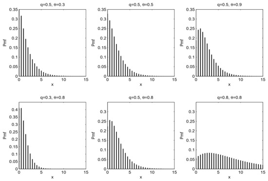
Figure 1. Plots of the pmf of the TRTG distribution for some choices of q and $\theta$.

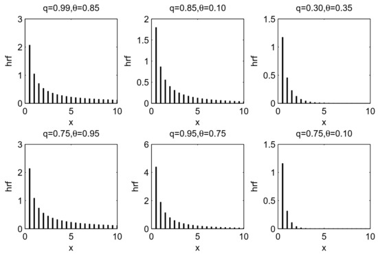
Figure 2. Plots of the hf of the TRTG distribution for some choices of q and $\theta$.

3. Distributional Properties

3.1. Moments and Quantile Function

The moment generating function of the TRTG distribution takes the form:

$$\begin{array}{ccc}\hfill M_X\left(t\right)& =& E\left(e^{tX}\right)\hfill \\ & =& \sum _{x=0}^{\infty }{e}^{tx}{q}^{\left(x+1\right)}\left(\theta log\left(q^{\left(x+1\right)}\right)-1\right)+q^x\left(\theta log\left(q^x\right)-1\right)\hfill \\ & =& \frac{qexp\left(t\right)\left(q-1-\theta log\left(q\right)\right)+1-q+\theta qlog\left(q\right)}{{\left(qexp\left(t\right)-1\right)}^2}.\hfill \end{array}$$

Note that by using $M_X\left(t\right)$, we can obtain the probability generating function of the TRTG distribution as follows:

$$\begin{array}{ccc}\hfill {\psi }_X\left(t\right)& =& E\left(t^X\right)\hfill \\ & =& M_X(ln\left(t\right))\hfill \\ & =& \frac{-q\theta \left(t-1\right)log\left(q\right)+\left(q-1\right)\left(qt-1\right)}{{\left(qt-1\right)}^2}.\hfill \end{array}$$

Hence, the first fourth moments of X can be derived as

$$\begin{array}{ccc}\hfill E\left(X\right)& =& \sum _{x=0}^{\infty }x{q}^{\left(x+1\right)}\left(\theta log\left(q^{\left(x+1\right)}\right)-1\right)+q^x\left(\theta log\left(q^x\right)-1\right)\hfill \\ & =& \frac{q\left(1-q-\theta log\left(q\right)\right)}{{\left(1-q\right)}^2},\hfill \end{array}$$

(8)

$$\begin{array}{ccc}\hfill E\left(X^2\right)& =& \sum _{x=0}^{\infty }{x}^2{q}^{\left(x+1\right)}\left(\theta log\left(q^{\left(x+1\right)}\right)-1\right)+q^x\left(\theta log\left(q^x\right)-1\right)\hfill \\ & =& \frac{q\left(q^2+3q\theta log\left(q\right)+\theta log\left(q\right)-1\right)}{\left(q-1\right){\left(1-q\right)}^2},\hfill \end{array}$$

$$\begin{array}{ccc}\hfill E\left(X^3\right)& =& \sum _{x=0}^{\infty }{x}^3{q}^{\left(x+1\right)}\left(\theta log\left(q^{\left(x+1\right)}\right)-1\right)+q^x\left(\theta log\left(q^x\right)-1\right)\hfill \\ & =& -\frac{(q^3+7q^2\theta log\left(q\right)+3q^2+10q\theta log\left(q\right)-3q+\theta log\left(q\right)-1)q}{{(q-1)}^4}\hfill \end{array}$$

and:

$$\begin{array}{ccc}\hfill E\left(X^4\right)& =& \sum _{x=0}^{\infty }{x}^4{q}^{\left(x+1\right)}\left(\theta log\left(q^{\left(x+1\right)}\right)-1\right)+q^x\left(\theta log\left(q^x\right)-1\right)\hfill \\ & =& \frac{15q^4\theta log\left(q\right)+55q^3\theta log\left(q\right)+q^5}{{(q-1)}^5}\hfill \\ & & +\frac{25q^2\theta log\left(q\right)+10q^4-10q^2+q\theta log\left(q\right)-q}{{(q-1)}^5}.\hfill \end{array}$$

Then, the variance, skewness, and kurtosis of X are given by

$$\begin{array}{ccc}\hfill Var\left(X\right)& =& E\left(X^2\right)-E{\left(X\right)}^2\hfill \\ & =& \frac{q\left[{\left(q-1\right)}^2+\left(q^2-1\right)\theta log\left(q\right)-{\theta }^{2}qlog{\left(q\right)}^2\right]}{{\left(q-1\right)}^4},\hfill \end{array}$$

$$\begin{array}{ccc}\hfill {\gamma }_1\left(X\right)& =& \frac{E{(X-E\left(X\right))}^3}{{\left[E{(X-E\left(X\right))}^2\right]}^{\frac{3}{2}}}\hfill \\ & =& -\frac{2{\theta }^{3}log{\left(q\right)}^3{q}^2+(-3{\theta }^2{q}^3+3q{\theta }^2)log{\left(q\right)}^2}{{(q-1)}^6}\hfill \\ & & +\frac{\theta (4q+q^2+1){(q-1)}^{2}log\left(q\right)+(q+1){(q-1)}^3}{{(q-1)}^6}\hfill \end{array}$$

and:

$$\begin{array}{ccc}\hfill {\gamma }_2\left(X\right)& =& \frac{E{(X-E\left(X\right))}^4}{{\left[E{(X-E\left(X\right))}^2\right]}^2}-3\hfill \\ & =& \left\{\frac{-3q^3{\theta }^{4}log{\left(q\right)}^4+(-6{\theta }^3{q}^2+6q^4{\theta }^3)log{\left(q\right)}^3-4{(q-1)}^2(q^2+\frac{11}{2}q+1)q{\theta }^{2}log{\left(q\right)}^2}{q{(-q{\theta }^{2}log{\left(q\right)}^2+(q^2\theta -\theta )log\left(q\right)+{(q-1)}^2)}^2}\right.\hfill \\ & & \left.+\frac{\theta (q+1)(q^2+16q+1){(q-1)}^{3}log\left(q\right)+(q^2+7q+1){(q-1)}^4}{q{(-q{\theta }^{2}log{\left(q\right)}^2+(q^2\theta -\theta )log\left(q\right)+{(q-1)}^2)}^2}\right\}-3.\hfill \end{array}$$

The quantile function (qf) of the TRTG distribution is derived as

$$Q\left(u\right) =-\frac{1+W\left(\frac{u-1}{\theta exp\left(1/\theta \right)}\right)\theta -\theta log\left(q\right)}{\theta log\left(q\right)},$$

(9)

where W refers to the Lambert function. From Equation (9), the $a^{th}$ quantile, $\left(x_a\right)$, of TRTG distribution is written by

$$x_a= \left\{\begin{array}{ccc}⌊\frac{1+W\left(\frac{u-1}{\theta exp\left(1/\theta \right)}\right)\theta -\theta log\left(q\right)}{\theta log\left(q\right)}⌋+1& ,& ⌊Q\left(a\right)⌋ \ne Q\left(a\right)\\ \left\{⌊\frac{1+W\left(\frac{u-1}{\theta exp\left(1/\theta \right)}\right)\theta -\theta log\left(q\right)}{\theta log\left(q\right)}⌋,⌊\frac{1+W\left(\frac{u-1}{\theta exp\left(1/\theta \right)}\right)\theta -\theta log\left(q\right)}{\theta log\left(q\right)}⌋+ 1\right\}& ,& ⌊Q\left(a\right)⌋ =Q\left(a\right)\end{array}\right.,$$

where $⌊x⌋$ denotes the integer part of x. That is, $x_a$ satisfies $F\left(x_a^{-}\right)\le p\le F\left(x_a\right),$ where F is the cdf (5) of the TRTG distribution. The median of the TRTG distribution follows by simply equating a with $0.5$.

The most important measure of any discrete distribution is the dispersion index (DI) which is defined as $DI=Var\left(X\right)/E\left(X\right)$. Some statistical measures of the TRTG distribution are computed and reported in Table 1. To interpret the individual effects of the parameters $\theta$ and q, the results are calculated for fixed $\theta =0.5$ and $q=0.5$. As seen from Table 1, the mean, variance, and DI are increasing functions of the parameter q for fixed $\theta =0.5$. In addition, the mean and variance are increasing functions of $\theta$ for fixed $q=0.5$. The DI decreases when the parameter $\theta$ increases. Furthermore, the results show that the TRTG distribution is suitable for over-dispersed count data.

Table 1. Some numerical measures of the TRTG model for $\theta =0.5$ and $q=0.5$.

	q
Measure	0.01	0.1	0.2	0.3	0.4	0.5	0.6	0.7	0.8	0.9
Mean	0.034	0.253	0.501	0.797	1.176	1.693	2.458	3.720	6.231	13.741
Variance	0.034	0.277	0.626	1.161	2.040	3.599	6.664	13.714	35.104	157.600
DI	1.007	1.094	1.249	1.456	1.735	2.126	2.713	3.686	5.633	11.469
	$\theta$
	0.01	0.1	0.2	0.3	0.4	0.5	0.6	0.7	0.8	0.9
Mean	1.014	1.139	1.277	1.416	1.554	1.693	1.832	1.970	2.109	2.248
Variance	2.041	2.397	2.755	3.075	3.356	3.599	3.803	3.970	4.097	4.186
DI	2.013	2.105	2.157	2.172	2.159	2.126	2.076	2.015	1.943	1.862

3.2. Stochastic Orders

Shaked and Shanthikumar [16] illustrated that several stochastic orders exist and have many applications. Stochastic orders are important measures to judge comparative behaviors of random variables.

The following theorem illustrates that the TRTG distribution is ordered according to the likelihood ratio ($lr$) order as the strongest stochastic order.

Theorem 1.

If X∼TRTG$\left(q,{\theta }_1\right)$ and $Y\sim$TRTG$\left(q,{\theta }_2\right)$. Then X ${<}_{lr}Y$ for all ${\theta }_1<{\theta }_2$.

Proof. 

The pmf of X can be expressed as

$$f\left(x\right) =\stackrel{W_1\left(x\right)}{\overbrace{q^{x+1}\left[\theta log\left(q^{x+1}\right)-1\right]}}+\stackrel{W_2\left(x\right)}{\overbrace{q^x\left[\theta log\left(q^x\right)-1\right]}}.$$

The density ratio of TRTG distribution, say $W\left(x\right)$, is obtained in two parts, as $W_1\left(x\right)$ and $W_2\left(x\right)$. If the two ratios, $W_1\left(x\right)$ and $W_2\left(x\right)$, are decreasing functions in x, then the density ratio, $W\left(x\right)$, is also a decreasing function of x. Then, $W_1\left(x\right)$ and $W_2\left(x\right)$ can be expressed as

$$W_1\left(x\right) =\frac{g_1\left(x;q,{\theta }_1\right)}{g_1\left(x;q,{\theta }_2\right)}=\frac{{\theta }_{1}log\left(q^{x+1}\right)-1}{{\theta }_{2}log\left(q^{x+1}\right)-1}$$

and:

$$W_2\left(x\right) =\frac{g_2\left(x;q,{\theta }_1\right)}{g_2\left(x;q,{\theta }_2\right)}=\frac{{\theta }_{1}log\left(q^x\right)-1}{{\theta }_{2}log\left(q^x\right)-1}.$$

Firstly, the first derivative of $W_1\left(x\right)$ with respect to x is given by

$$W_1^{\prime }\left(x\right) =-\frac{log\left(q\right)\left({\theta }_1-{\theta }_2\right)}{\underset{>0}{\underbrace{{\left[{\theta }_{2}log\left(q^{x+1}\right)-1\right]}^2}}},$$

where $\left({\theta }_1-{\theta }_2\right) <0$ for ${\theta }_1<{\theta }_2$. Hence, $W_1^{\prime }\left(x\right) <0$ for ${\theta }_1<{\theta }_2$.

Similarly, the first derivative of $W_2\left(x\right)$ with respect to x has the form:

$$W_2^{\prime }\left(x\right) =-\frac{log\left(q\right)\left({\theta }_1-{\theta }_2\right)}{\underset{>0}{\underbrace{{\left[{\theta }_{2}log\left(q^x\right)-1\right]}^2}}},$$

where $\left({\theta }_1-{\theta }_2\right) <0$ for ${\theta }_1<{\theta }_2$. Then, $W_2^{\prime }\left(x\right) <0$ for ${\theta }_1<{\theta }_2$. It is seen that both density ratios, $W_1\left(x\right)$ and $W_2\left(x\right)$, are decreasing functions in x. Hence, $W\left(x\right) =W_1\left(x\right)+W_2\left(x\right)$ is also a decreasing function in x. The proof is completed. □

Based on the chain of stochastic orders (see, [16] and Definition 4 in [7]), we conclude that the TRTG distribution can be ordered according to the hazard rate ($hr$), reversed hazard rate ($rh$), mean residual life ($mrl$), and stochastic ($st$) orders. That is, X ${<}_{hr}Y$, X ${<}_{rh}Y$, X ${<}_{mrl}Y$, and X ${<}_{st}Y$.

3.3. Mean Deviation and Mean Residual Life

The mean deviation ($MD$) of the TRTG model is derived as

$$\begin{array}{ccc}\hfill MD& =& \sum _{x=0}^{t}xp\left(x\right)\hfill \\ & =& \sum _{x=0}^{t}x\left(q^{\left(x+1\right)}\left(\theta log\left(q^{\left(x+1\right)}\right)-1\right)-q^x\left(\theta log\left(q^x\right)-1\right)\right)\hfill \\ & =& \frac{q^{(t+2)}t+q^{(t+2)}-q^{(t+3)}t-q^2-q^{(t+1)}t-q^{(t+1)}+q^{(t+2)}t+q}{{(-1+q)}^2}\hfill \\ & & +\left(\sum _{x=0}^t\left(x{q}^{(x+1)}\theta log\left(q^{(x+1)}\right)-x{q}^x\theta log\left(q^x\right)\right)\right).\hfill \end{array}$$

The $mrl$ of the TRTG model is defined by

$$\begin{array}{ccc}\hfill m\left(x\right)& =& \frac{{\displaystyle \sum _{k=x+1}^{\infty }}S\left(k\right)}{S\left(x\right)}\hfill \\ & =& \frac{1-{\sum }_{k=0}^x\left(-q^k\theta log\left(q^k\right)+q^k\right)}{\left(-q^x\theta log\left(q^x\right)+q^x\right)}\hfill \\ & =& \frac{(q-1){\sum }_{k=0}^x\left(-q^k\theta log\left(q^k\right)\right)-q+q^{(x+1)}}{(q-1)q^x(\theta log\left(q^x\right)-1)}.\hfill \end{array}$$

4. Actuarial Measures

In this section, we determined the value at risk (VaR) and tail value at risk (TVaR) measures of the TRTG distribution.

4.1. VaR Measure of the TRTG Distribution

Let X denote a loss random variable. The VaR${}_{\alpha }$ of X at the $100\alpha \%$ level, denoted by ${\pi }_{\alpha }$, is the $100\alpha$ percentile (or quantile) of the distribution of X. Hence, the VaR${}_{\alpha }$ of the TRTG model is defined by

$$\begin{array}{ccc}\hfill P\left(X>{\pi }_{\alpha }\right)& =& 1-\alpha \hfill \\ \hfill {\pi }_{\alpha }& =& F^{-1}\left(\alpha \right),\hfill \end{array}$$

where $\alpha \in \left(0,1\right)$ and F is the cdf of the TRTG distribution given in (5). The VaR${}_{\alpha }$ of the TRTG distribution with qf (9) is derived as

$${\pi }_p=\frac{1+W\left(\frac{\alpha -1}{\theta exp\left(1/\theta \right)}\right)\theta -\theta log\left(q\right)}{\theta log\left(q\right)}.$$

4.2. TVaR Measure of the TRTG Distribution

Let X denote a loss random variable. The TVaR of X at the $100\alpha \%$ security level, denoted by TVaR${}_{\alpha }$ is the expected loss given that the loss exceeds the $100\alpha$ percentile of the distribution of X. For engineering or actuarial applications, it is more common to consider the distribution of losses—in this case the right-tail TVaR is considered (typically for $\alpha =95\%$ or $\alpha =99\%$). The TVAR${}_{\alpha }$ is defined by

$$TVa{R}_{\alpha }=E\left(X\mid X>{\pi }_{\alpha }\right) =\frac{{\displaystyle \sum _{x={\pi }_{\alpha }}^{\infty }}xf\left(x\right)}{1-F\left({\pi }_{\alpha }\right)}.$$

Using the pmf and cdf of the TRTG model, the TVaR${}_{\alpha }$ is derived as

$$\begin{array}{ccc}\hfill TVa{R}_{\alpha }& =& E\left(X\mid X>{\pi }_{\alpha }\right)\hfill \\ & =& \frac{1}{1-\alpha }\sum _{x={\pi }_{\alpha }}^{\infty }x{q}^{\left(x+1\right)}\left(\theta log\left(q^{\left(x+1\right)}\right)-1\right)+q^x\left(\theta log\left(q^x\right)-1\right).\hfill \end{array}$$

Table 2 provides some numerical computations for the VaR${}_{\alpha }$ and TVaR${}_{\alpha }$ measures of the TRTG$\left(q,\theta \right)$ distribution for different parametric values.

Table 2. Numerical values of VaR${}_{\alpha }$ and TVaR${}_{\alpha }$ measures of the TRTG distribution.

$\mathit{\theta }$	q	Security Level	VaR${}_{\mathit{\alpha }}$	TVaR${}_{\mathit{\alpha }}$
0.25	0.25	0.90	1.0478	2.5654
		0.95	1.6280	5.1309
		0.99	2.9433	10.8642
0.25	0.50	0.90	3.0957	11.0154
		0.95	4.2561	7.2157
		0.99	6.8867	2.8204
0.25	0.75	0.90	8.8682	15.4903
		0.95	11.6642	9.1255
		0.99	18.0024	2.2378
0.50	0.25	0.90	1.3601	3.6725
		0.95	1.9669	7.3451
		0.99	3.3210	6.5062
0.75	0.25	0.90	1.6067	4.7797
		0.95	2.2213	4.4352
		0.99	3.5860	8.9130

5. Estimation

In this section, the estimation of the TRTG parameters is examined using some classical and Bayesian methods.

5.1. Method of Maximum Likelihood

Let $x_1,\dots ,x_n$ be the observations of n independent and identically random variables $X_1,\dots ,X_n$ from the TRTG distribution. Then, the corresponding log-likelihood function reduces to:

$$\begin{array}{ccc}\hfill {\ell }_n(q,\theta )& =& logq\sum _{i=0}^n{x}_i+\sum _{i=0}^{n}log\left[\left(\theta qlog{q}^{x_i+1}-q\right)-\left(\theta log{q}^{x_i}-1\right)\right].\hfill \end{array}$$

Then, the maximum likelihood (ML) estimators of q and $\theta$, say $\widehat{q}$ and $\widehat{\theta }$, are the solution of the following linear equations: $\partial {\ell }_n(q,\theta )/\partial q=0$ and $\partial {\ell }_n(q,\theta )/\partial \theta =0$. The ML estimators of q and $\theta$ cannot be obtained explicitly. Therefore, they can be obtained by numerical methods. The fminsearch command in Matlab is used for this purpose.

5.2. Method of Moments

The moments (MM) estimators of the parameters $q$ and $\theta$ were obtained by simultaneously solving the following two equations:

$$\frac{q\left(1-q-\theta logq\right)}{{\left(1-q\right)}^2}=\frac{1}{n}\sum _{i=1}^n{X}_i$$

(10)

and:

$$\frac{q\left(q^2+3q\theta logq+\theta logq-1\right)}{\left(q-1\right){\left(1-q\right)}^2}=\frac{1}{n}\sum _{i=1}^n{X}_i^2.$$

(11)

Equations (10) and (11) can be numerically solved using the Newton–Raphson method. The solutions of these two equations are the MM estimators of the parameters q and $\theta$.

5.3. Method of Proportions

The method of proportions is proposed by [17] to estimate the parameters of discrete Weibull distribution. Then, we used this method to estimate the TRTG parameters. Let $X_1,X_2,\dots ,X_n$ be a random sample from the TRTG$\left(q,\theta \right)$ distribution. Consider the indicator function, say $\nu (.)$, which is defined (for $i=1,2,\dots ,n$) as

$$\nu \left(X_i\right) = \left\{\begin{array}{c}1,X_i=0\\ 0,X_i>0\end{array}\right.,i=1,2,\dots ,n.$$

Then, $Y=\frac{1}{n}{\displaystyle \sum _{i=1}^n}\upsilon \left(X_i\right)$ denotes the proportion of zeros in the sample and estimates the probability $f\left(0\right) =q\left(\theta logq-1\right) + 1$. Similarly, Z denotes the proportion of ones in the sample and it estimates the probability $f\left(1\right) =q^2\left(\theta log{q}^2-1\right) - q\left(\theta log\left(q\right) - 1\right)$. Hence, the proportions (MP) estimators of parameters $q$ and $\theta$ are obtained by solving the following two equations simultaneously:

$$\begin{array}{ccc}\hfill q\left(\theta logq-1\right) + 1& =& Y\hfill \end{array}$$

(12)

and:

$$\begin{array}{ccc}\hfill q^2\left(\theta log{q}^2-1\right) - q\left(\theta log\left(q\right) - 1\right)& =& Z.\hfill \end{array}$$

(13)

Equations (12) and (13) can be numerically solved using the Newton–Raphson method. The solutions of the last two equations represent the MP estimators of the parameters q and $\theta$.

5.4. Bayesian Method

To obtain the Bayes estimators of the parameters q and $\theta$, we suppose that q has a beta distribution with parameters ${\alpha }_1$ and ${\beta }_1$ and $\theta$ has a beta distribution with parameters ${\alpha }_2$ and ${\beta }_2$ and q and $\theta$ are independent. Then, the prior density functions of q and $\theta$ are given by

$${\pi }_1\left(q\right)=\frac{1}{B({\alpha }_1,{\theta }_1)}{q}^{{\alpha }_1-1}{(1-q)}^{{\beta }_1-1},p\in (0,1)$$

and:

$${\pi }_2\left(\theta \right)=\frac{1}{B({\alpha }_2,{\theta }_2)}{\theta }^{{\alpha }_2-1}{(1-\theta )}^{{\beta }_2-1},\theta \in (0,1),$$

respectively, where $\beta \left(·,·\right)$ is the beta function. Therefore, the joint prior of $\left(q,\theta \right)$ can be expressed as

$$\pi (q,\theta )={\pi }_1\left(q\right){\pi }_2\left(\theta \right)=\frac{1}{B({\alpha }_1,{\theta }_1)B({\alpha }_2,{\theta }_2)}{q}^{{\alpha }_1-1}{(1-q)}^{{\beta }_1-1}{\theta }^{{\alpha }_2-1}{(1-\theta )}^{{\beta }_2-1}.$$

Under the squared error loss function, the Bayes estimators of q and $\theta$ can be expressed as

$$\begin{array}{ccc}\hfill \widehat{q}& =& E\left(q\right|x)=\frac{\underset{0}{\overset{1}{\int }}\underset{0}{\overset{1}{\int }}qL(q,\theta /x)\pi (q,\theta )dqd\theta }{\underset{0}{\overset{1}{\int }}\underset{0}{\overset{1}{\int }}L(q,\theta /x)\pi (q,\theta )dqd\theta }\hfill \\ \hfill \mathrm{and}:\\ \hfill \hat{\theta }& =& E\left(\theta \right|x)=\frac{\underset{0}{\overset{1}{\int }}\underset{0}{\overset{1}{\int }}\theta L(q,\theta /x)\pi (q,\theta )dqd\theta }{\underset{0}{\overset{1}{\int }}\underset{0}{\overset{1}{\int }}L(q,{\hat{\theta }}_2/x)\pi (q,{\hat{\theta }}_2)dqd{\hat{\theta }}_2},\hfill \end{array}$$

respectively. These estimators cannot be explicitly obtained but they can be approximately obtained by using Tierney and Kadene’s (1986) method [18].

6. Simulation Study

To obtain information about the performance of the previous estimators, we conducted an appropriate simulation study. In this simulation, we generated samples of size $n=100,200,300,400,500,1000$ from the TRTG$(q,\theta )$ distribution and then computed the ML, MM, MP, and Bayes estimates of q and $\theta$. We calculated the average absolute biases (ABBs), mean square errors (MSEs), and mean relative errors of the estimates (MREs) for all methods. The ABBs, MREs, and MSEs are calculated by

$${\widehat{ABBs}}_{\phi }=\frac{1}{N}{\sum }_{i=1}^N\left|\hat{\phi }-\phi \right|,$$

$${\widehat{MSE}}_{\phi }=\frac{1}{N}{\sum }_{i=1}^N{\left(\hat{\phi }-\phi \right)}^2$$

and:

$${\widehat{MRE}}_{\phi }=\frac{1}{N}{\sum }_{i=1}^N\left|\hat{\phi }-\phi \right|/\phi ,$$

where $\phi =\left(\theta ,q\right)$ and $\hat{\phi }=\left(\widehat{\theta },\widehat{q}\right)$.

The optim-CG routine in the R program were adopted to generate 5000 trials to estimate these indices of the ML, MM, MP, and Bayes estimates. Different sample sizes and two-parameter settings were considered, $\left(\theta =0.5,q=0.4\right)$ and $\left(\theta =0.6,q=0.5\right)$. The results are given in Table 3 and Table 4. From Table 3 and Table 4, it was concluded that the ABBs, MREs and MSEs of all estimates decrease when n increases as expected. Moreover, the Bayes, ML, and MM methods provide the best estimates in terms of performance criteria. The Bayes, ML and MM estimates are almost identical in terms of ABBs, MSEs, and MREs and they perform better than the MP estimates. Furthermore, as the sample size n increases, the ABBs and MSEs of all estimators reduce as expected.

Table 3. Simulation results of the TRTG model for $\theta =0.5$ and $q=0.4$.

		ML		MP		MM		Bayes
$\mathit{n}$		$\mathit{\theta }$	$\mathit{q}$	$\mathit{\theta }$	$\mathit{q}$	$\mathit{\theta }$	$\mathit{q}$	$\mathit{\theta }$	$\mathit{q}$
100	MSEs	0.0253	0.0035	0.0369	0.0656	0.0416	0.0896	0.0209	0.0008
	ABBs	0.1592	0.0589	0.1922	0.2561	0.2994	0.5098	0.1445	0.0290
	MREs	0.3183	0.1473	0.3843	0.6402	0.5098	0.7485	0.2890	0.0726
200	MSEs	0.0139	0.0019	0.0244	0.0538	0.0208	0.0574	0.0149	0.0005
	ABBs	0.1177	0.0436	0.1561	0.2319	0.1442	0.2395	0.1221	0.0226
	MREs	0.2355	0.1090	0.3122	0.5797	0.3605	0.5988	0.2442	0.0564
300	MSEs	0.0091	0.0013	0.0177	0.0426	0.0134	0.0451	0.0103	0.0004
	ABBs	0.0954	0.0358	0.1332	0.2064	0.1157	0.2124	0.1014	0.0188
	MREs	0.1908	0.0894	0.2663	0.5160	0.2891	0.5311	0.2029	0.0470
400	MSEs	0.0065	0.0010	0.0127	0.0360	0.0101	0.0388	0.0078	0.0003
	ABBs	0.0804	0.0310	0.1128	0.1897	0.1003	0.1971	0.0884	0.0171
	MREs	0.1608	0.0774	0.2256	0.4743	0.2508	0.4926	0.1768	0.0428
500	MSEs	0.0051	0.0008	0.0107	0.0323	0.0077	0.0343	0.0049	0.0007
	ABBs	0.0713	0.0276	0.1036	0.1798	0.0876	0.1852	0.0698	0.0278
	MREs	0.1425	0.0690	0.2071	0.4495	0.2189	0.4631	0.1429	0.0678
1000	MSEs	0.0026	0.0004	0.0053	0.0236	0.0037	0.0251	0.0023	0.0003
	ABBs	0.0513	0.0200	0.0728	0.1535	0.0608	0.1585	0.0476	0.0186
	MREs	0.1025	0.0499	0.1456	0.3837	0.1521	0.3963	0.1031	0.0510

Table 4. Simulation results of the TRTG model for $\theta =0.6$ and $q=0.5$.

		ML		MP		MM		Bayes
$\mathit{n}$		$\mathit{\theta }$	$\mathit{q}$	$\mathit{\theta }$	$\mathit{q}$	$\mathit{\theta }$	$\mathit{q}$	$\mathit{\theta }$	$\mathit{q}$
100	MSEs	0.0220	0.0026	0.0424	0.0262	0.0318	0.0130	0.0159	0.0018
	ABBs	0.1482	0.0506	0.2058	0.1620	0.1782	0.1138	0.1262	0.0425
	MREs	0.2964	0.0844	0.4116	0.2699	0.2971	0.1897	0.2104	0.0850
200	MSEs	0.0111	0.0012	0.0277	0.0156	0.0152	0.0055	0.0091	0.0008
	ABBs	0.1052	0.0353	0.1665	0.1249	0.1233	0.0743	0.0954	0.0274
	MREs	0.2105	0.0589	0.3331	0.2082	0.2055	0.1239	0.1590	0.0549
300	MSEs	0.0074	0.0009	0.0213	0.0122	0.0104	0.0040	0.0060	0.0004
	ABBs	0.0862	0.0299	0.1458	0.1106	0.1019	0.0634	0.0774	0.0199
	MREs	0.1726	0.0498	0.2917	0.1843	0.1698	0.1057	0.1290	0.0397
400	MSEs	0.0051	0.0006	0.0164	0.0094	0.0078	0.0034	0.0046	0.0004
	ABBs	0.0711	0.0249	0.1280	0.0969	0.0882	0.0579	0.0632	0.0212
	MREs	0.1423	0.0415	0.2559	0.1615	0.1471	0.0966	0.1142	0.0424
500	MSEs	0.0043	0.0005	0.0140	0.0084	0.0062	0.0031	0.0028	0.0002
	ABBs	0.0655	0.0224	0.1182	0.0917	0.787	0.0556	0.0498	0.0196
	MREs	0.1311	0.0374	0.2364	0.1529	0.1312	0.0926	0.1087	0.0265
1000	MSEs	0.0020	0.0002	0.0081	0.0057	0.0031	0.0028	0.0016	0.0002
	ABBs	0.0448	0.0156	0.0898	0.0756	0.0557	0.0526	0.0364	0.0127
	MREs	0.0896	0.0260	0.1795	0.1259	0.1114	0.0877	0.0638	0.0172

7. Modeling Three Actuarial Data

In this section, the TRTG distribution was fitted into three real actuarial data sets and compared with the transmuted geometric (TRAG), discrete Burr (DB), discrete Chen (DC), negative binomial (NB), geometric (G), and Poisson (P) distributions.

First data set: These data were reported in Klugman et al. [19] and represent the number of claims of automobile liability policies.

Second data set: The data were analyzed by Klugman et al. [19] and represent the number of hospitalizations per family member and year.

Third data set: These data were studied by Willmot [20] and refer to the number of automobile insurance claims per policy in two portfolios from Belgium during the period 1975–1976, respectively.

The TRTG, TRAG, DB, DC, NB, G, and P distributions were fitted to the three data sets, respectively. Their parameters estimates were obtained via the ML method. The chi-square procedure was adopted to test $H_0:X\sim$ TRTG$(q,\theta )$. To compute the ${\chi }^2$ statistic, the unknown parameters q and $\theta$ were estimated from the three data sets. Under null hypothesis, the estimated probabilities can be calculated by

$$\widehat{P}(X=i)={\widehat{q}}^{\left(i+1\right)}\left(\widehat{\theta }log\left({\widehat{q}}^{\left(i+1\right)}\right)-1\right)-{\widehat{q}}^i\left(\widehat{\theta }log\left({\widehat{q}}^i\right)-1\right),i=0,1,...$$

and the estimated expected frequencies are $\widehat{e_i}=n\widehat{{\alpha }_i},$ where $\hat{\alpha }$ is an ML estimate of $\alpha$. For the three data sets, the chi-square test, ${\chi }^2$, was computed for the TRTG distribution and other competing distributions. The results of observed and expected frequencies, ${\chi }^2$ and $-{\ell }_n$ are listed in Table 5, Table 6 and Table 7 for the three data sets, respectively. The values in these tables reveal that the TRTG distribution has the lowest values for ${\chi }^2$ and $-{\ell }_n$ among all competing discrete models and it provides a better fit for the given data sets than the TRAG, DB, DC, NB, G, and P distributions. Based on the results, we cannot reject $H_0$ at the $\alpha =0.05$ significance level.

Table 5. Results of observed and expected frequencies, ${\chi }^2$ and $-{\ell }_n$, respectively, for first data.

Count	Observed	Expected
		TRTG	NB	TRAG	DB	DC	G	P
0	99	96.65	95.86	96.32	101.65	108.84	110.06	54.01
1	65	74.30	75.83	75.71	93.25	59.82	69.41	92.24
2	57	50.24	50.35	50.24	39.88	44.86	43.78	78.77
3	35	31.71	31.3	31.10	19.60	32.56	27.61	44.85
4	20	19.18	18.79	18.61	11.15	22.20	17.41	19.15
5	10	11.26	11.04	10.94	7.03	14.01	10.98	6.54
≥6	12	9.98	10.02	10.13	15.51	15.64	12.13	1.97
Total	$n=$ 298
Parameters	$\widehat{q}$	0.5019	0.4606	0.5748	0.5478	0.7676	0.3693
	$\widehat{\theta }$	0.5022	1.4590	−0.4172	2.2728	0.5104		1.7080
	${\chi }^2$	3.09	3.58	3.55	30.09	7.10	6.60	297.53
	$-{\ell }_n$	528.62	528.77	528.73	551.45	532.82	531.46	577.01

Table 6. Results of observed and expected frequencies, ${\chi }^2$ and $-{\ell }_n$, respectively, for second data.

Count	Observed	Expected
		TRTG	NB	TRAG	DB	DC	G	P
0	96,978	96,966.54	97,038.57	97,031.24	96,974.15	97,008.08	97,148.31	96,684.62
1	9240	9252.80	9080.28	9129.30	9290.98	9145.87	8923.19	9777.85
2	704	703.06	783.53	747.53	611.61	786.07	819.61	494.42
3	43	48.25	65.71	60.58	76.24	33.40	75.28	16.67
4	9	3.12	5.43	4.9	14.9	0.50	6.91	0.42
Total	$n=$ 106,974
Parameters	$\widehat{q}$	0.0523	0.9209	0.0810	0.0327	0.2512	0.9081
	$\widehat{\theta }$	0.2668	1.1844	−0.1609	1.7386	0.5945		0.1011
	${\chi }^2$	4.50	25.19	13.10	41.97	20.71	54.86	118.89
	$-{\ell }_n$	36,021.61	36,111.66	36,104.30	36,123.01	36,122.60	36,123.59	36,188.25

Table 7. Results of observed and expected frequencies, ${\chi }^2$ and $-{\ell }_n$, respectively, for third data.

Count	Observed	Expected
		TRTG	NB	TRAG	DB	DC	G	P
0	2659	2658.92	2660.38	2659.03	2658.88	2659.68	2661.70	2649.90
1	244	243.98	241.05	243.65	245.29	241.56	238.77	260.80
2	19	19.53	20.67	19.48	16.98	21.70	21.42	12.80
≥3	2	1.46	1.74	1.42	2.21	1.04	1.92	0.42
Total	$n=$ 2924
Parameters	$\widehat{q}$	0.0545	0.9191	0.0799	0.0313	0.2469	0.0896
	$\widehat{\theta }$	0.2280	11.1960	−0.1489	1.6911	0.5827		0.0984
	${\chi }^2$	0.16	0.22	0.18	0.24	0.87	0.43	4.44
	$-{\ell }_n$	967.24	969.12	969.06	969.62	969.42	969.25	972.26

Furthermore, for visual comparisons, the observed and fitted distributions are displayed in Figure 3, Figure 4 and Figure 5 for the three data sets, respectively.

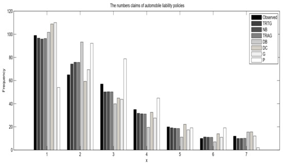
Figure 3. Observed and fitted distributions for first data.

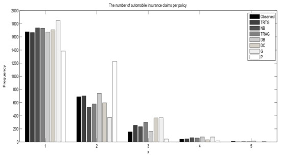
Figure 4. Observed and fitted distributions for second data.

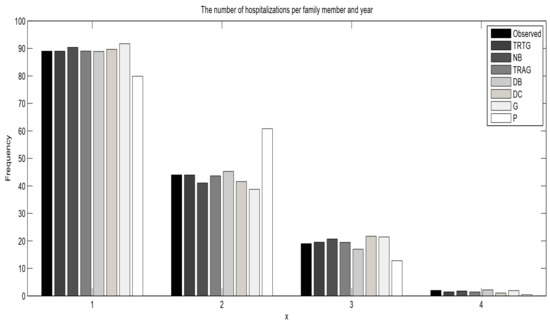
Figure 5. Observed and fitted distributions for third data.

8. TRTG Count Regression Model

Let X be the response variable and $\mathbf{y}$ be its associated $p\times 1$ vector of covariates. Assume that the response variable X follows the TRTG distribution with the mean $\mu \left(y\right)$. Furthermore, the mean of the response variable linked with the explanatory variables by log-linear form, i.e., ${\mu }_i=exp\left(\mathit{\beta }{\mathbf{y}}_i^T\right)$, where $\mathit{\beta }= \left({\beta }_1,{\beta }_2,\dots ,{\beta }_p\right)$ and ${\mathbf{y}}_i= \left(1,y_{1i},y_{2i},\dots ,y_{pi}\right).$ by replacing $\theta$ with $\frac{\left(1-q\right)\left(\left(1+{\mu }_i\right)q-{\mu }_i\right)}{qlogq}$, we obtain the re-parameterized pmf of Equation (6) as

$$\begin{array}{ccc}\hfill p\left(x_i\right)& =& q^{\left(x_i+1\right)}\left(\left(\frac{\left(1-q\right)\left(\left(1+{\mu }_i\right)q-{\mu }_i\right)}{qlogq}\right)log\left(q^{\left(x_i+1\right)}\right)-1\right)\hfill \\ & & -q^{x_i}\left(\left(\frac{\left(1-q\right)\left(\left(1+{\mu }_i\right)q-{\mu }_i\right)}{qlogq}\right)log\left(q^{x_i}\right)-1\right).\hfill \end{array}$$

The corresponding log-likelihood equation takes the form

$$\begin{array}{ccc}\hfill {\ell }_n(q,\theta )& =& logq\sum _{i=0}^n\left(x_i\right)\hfill \\ & & +\sum _{i=0}^{n}log\left[\left(\frac{\psi \left(q,{\mu }_i\right)}{logq}log{q}^{x_i+1}-q\right)-\left(\frac{\psi \left(q,{\mu }_i\right)}{logq}log{q}^{x_i}-1\right)\right],\hfill \end{array}$$

(14)

where $\psi \left(q,{\mu }_i\right)=\left(1-q\right)\left(\left(1+{\mu }_i\right)q-{\mu }_i\right)$. Equation (14) is not in closed form and it cannot be solved explicitly. Some numerical methods can be used to achieve solutions. We illustrate the application of TRTG regression model by analyzing a real data about the count of infected blood cells (per mm2) on microscope slides prepared from $n=511$ randomly selected individuals [21]. The response variable ($x_i$: count of infected blood cells) was related to the following explanatory variables: the smoking status of the subject ($y_{i1}:$ 0: yes; 1: no), and their sex ($y_{i2}:$ 0: female; 1: male). Based on Table 8, we can strongly conclude that the proposed TRTG count regression model outperforms the Poisson, geometric, and PL regression models. The log-likelihood $\left({\widehat{\ell }}_{max}\right)$ and Akaike information criteria (AIC) are also reported in Table 8.

Table 8. Estimated parameters for the TRTG, Poisson, geometric, and PL regression models along with $\left({\widehat{\ell }}_{max}\right)$ and AIC.

Variable	Parameter	TRTG	PL	Geometric	Poisson
Intercept	${\beta }_1$	0.4508	0.6110	0.6573	0.5091
Smoking	${\beta }_2$	−1.0077	−0.8799	−0.9999	−1.1775
Gender	${\beta }_3$	0.1494	0.1956	1.9607	0.1846
Dispersion	$\varphi$	0.4654
${\widehat{\ell }}_{max}$		−632.16	−640.78	−685.59	−693.77
AIC		1272.32	1287.56	1377.18	1393.53

9. Conclusions

We derived and studied a new discrete distribution which was defined on $\mathbb{N}$ using the transmuted record type approach to extend the geometric distribution. The new model is called transmuted record type geometric (TRTG) distribution and it is suitable for over-dispersed count data. We introduced the distributional properties of the TRTG distribution along with two actuarial or risk measures. The TRTG parameters are discussed by four different estimation methods. A Monte Carlo simulation study was conducted to investigate the efficiency of different estimators. A new count regression model was proposed as an alternative count regression model for Poisson, geometric, and Poisson–Lindley regression models. In summary, the TRTG model can be considered as a good alternative to the negative binomial, geometric, and Poisson distributions. The TRTG distribution can be used to model insurance data as compared to the negative binomial, transmuted geometric, discrete Burr, discrete Chen, geometric, and Poisson distributions. The results show that the TRTG distribution outperforms some important discrete models.

References

- Chakaraborty, S.; Chakaraborty, D. Discrete gamma distribution: Properties and parameter estimation. Commun. Stat. Theory Methods 2012, 41, 3301–3324. [Google Scholar] [CrossRef]
- Nakagawa, T.; Osaki, S. Discrete Weibull distribution. IEEE Trans. Reliab. 1975, 24, 300–301. [Google Scholar] [CrossRef]
- Krishna, H.; Pundir, P.S. Discrete Burr and discrete Pareto distributions. Stat. Methodol. 2009, 6, 177–188. [Google Scholar] [CrossRef]
- Gómez-Déniz, E. A new discrete distribution: Properties and applications in medical care. J. Appl. Stat. 2013, 40, 2760–2770. [Google Scholar] [CrossRef]
- Akdoğan, Y.; Kuş, C.; Asgharzadeh, A.; Kınacı, I.; Shafari, F. Uniform-geometric distribution. J. Stat. Comput. Simul. 2016, 86, 1754–1770. [Google Scholar] [CrossRef]
- Kuş, C.; Akdoğan, Y.; Asgharzadeh, A.; Kınacı, I.; Karakaya, K. Binomial-discrete Lindley distribution. Commun. Fac. Sci. Univ. Ank. Ser. A1 Math. Stat. 2018, 68, 401–411. [Google Scholar] [CrossRef]
- Al-Babtain, A.A.; Ahmed, A.H.N.; Afify, A.Z. A new discrete analog of the continuous lindley distribution, with reliability applications. Entropy 2020, 22, 603. [Google Scholar] [CrossRef] [PubMed]
- Gómez-Déniz, E.; Calderın-Ojeda, E. The discrete Lindley distribution: Properties and applications. J. Stat. Comput. Simul. 2011, 81, 1405–1416. [Google Scholar] [CrossRef]
- Bakouch, H.S.; Jazi, M.A.; Nadarajah, S. A new discrete distribution. Statistics 2014, 48, 200–240. [Google Scholar] [CrossRef]
- Balakrishnan, N.; He, M. A Record-Based Transmuted Family of Distributions. In Advances in Statistics-Theory and Applications. Emerging Topics in Statistics and Biostatistics; Ghosh, I., Balakrishnan, N., Ng, H.K.T., Eds.; Springer: Cham, Switzerland, 2021. [Google Scholar]
- Shakil, M.; Ahsanullah, M. Record values of the ratio of Rayleigh random variables. Pak. J. Stat. 2011, 27, 307–325. [Google Scholar]
- Tanış, C.; Saraçoğlu, B. On the record-based transmuted model of balakrishnan and He based on Weibull distribution. Commun. Stat.-Simul. Comput. 2020. [Google Scholar] [CrossRef]
- Chakraborty, S.; Bhati, D. Transmuted geometric distribution with applications in modeling and regression analysis of count data. SORT 2016, 40, 153–176. [Google Scholar]
- Noughabi, M.S.; Rezaei Roknabadi, A.H.; Mohtashami Borzadaran, G.R. Some discrete lifetime distributions with bathtub-shaped hazard rate functions. Qual Eng. 2013, 25, 225–236. [Google Scholar] [CrossRef]
- Sankaran, M. The discrete Poisson-Lindley distribution. Biometrics 1970, 26, 145–149. [Google Scholar] [CrossRef]
- Shaked, M.; Shanthikumar, J.G. Stochastic Orders; Springer: New York, NY, USA, 2007. [Google Scholar]
- Khan, M.S.A.; Khalique, A.; Abouammoh, A.M. On estimating parameters in a discrete Weibull distribution. IEEE Trans. Reliab. 1989, 38, 348–350. [Google Scholar] [CrossRef]
- Tierney, L.; Kadene, J. Accurate approximation for posterior moments and marginal densities. J. Am. Stat. Assoc. 1986, 81, 82–86. [Google Scholar] [CrossRef]
- Klugman, S.; Panjer, H.; Willmot, G. Loss Models: From Data to Decisions; John Wiley & Sons: Hoboken, NJ, USA, 2012; Volume 715. [Google Scholar]
- Willmot, G.E. The Poisson-inverse Gaussian distribution as an alternative to the negative binomial. Scand. Actuar. J. 1987, 1987, 113–127. [Google Scholar] [CrossRef]
- Crawley, M.J. The R Book, 2nd ed.; John Wiley & Sons: New York, NY, USA, 2012. [Google Scholar]
Publisher’s Note: MDPI stays neutral with regard to jurisdictional claims in published maps and institutional affiliations. |
© 2021 by the authors. Licensee MDPI, Basel, Switzerland. This article is an open access article distributed under the terms and conditions of the Creative Commons Attribution (CC BY) license (https://creativecommons.org/licenses/by/4.0/).