Abstract
In this paper, we construct second-order weak split-step approximations of the CKLS and CEV processes that use generation of a three−valued random variable at each discretization step without switching to another scheme near zero, unlike other known schemes (Alfonsi, 2010; Mackevičius, 2011). To the best of our knowledge, no second-order weak approximations for the CKLS processes were constructed before. The accuracy of constructed approximations is illustrated by several simulation examples with comparison with schemes of Alfonsi in the particular case of the CIR process and our first-order approximations of the CKLS processes (Lileika– Mackevičius, 2020).
MSC:
60H35; 65C30
1. Introduction
We are interested in weak second-order approximations for the Chan–Karolyi– Longstaff–Sanders (CKLS) model [1]
with parameters , where and . In particular, when and , we have the constant elasticity of variance (CEV) model [2], and when and , we have the well-known Cox–Ingersoll–Ross (CIR) model [3]. The main problem in developing numerical methods for such a diffusion equation/model is that the diffusion coefficient has unbounded derivatives near zero, and therefore standard methods (see, e.g., Milstein and Tretyakov [4]) are not applicable: discretization schemes that (explicitly or implicitly) involve the derivatives of the coefficients usually lose their accuracy near zero, especially for large . This problem for the CIR processes was solved by modifying the scheme considered by switching near zero to another scheme, which is (1) sufficiently regular and (2) sufficiently accurate near zero; we refer, for example, to [5,6,7] and references therein. Typically, a second-order approximation near zero is constructed by discrete random variables matching three or four moments with those of the true solution.
The main result of this paper is the construction of second-order weak split-step approximations of the CKLS and CEV processes by discrete random variables. To the best of our knowledge, no second-order weak approximations of the CKLS process have been constructed before, except for the particular case of the CIR process (Alfonsi [5], Mackevičius [7]). Our construction method is significantly different from that of the first-order approximation in our previous paper [8]. Another novel feature of our result is that in our schemes, no switching between schemes near zero is used, in contrast to [5,7]. This simplifies the implementation of approximations. We illustrate the accuracy of our approximations by several simulation examples with comparison with schemes of Alfonsi in the particular case of the CIR process and our first-order approximations of the CKLS processes constructed in [8].
Why are second-order schemes better than first-order ones? On the one hand, the former are more accurate when using the same discretization step size. On the other hand, by the former, we can reach the same accuracy under larger step sizes, which implies lower computation costs. Of course, if high accuracy is not required, first-order approximations suffice.
The paper is organized as follows. In Section 2, we recall some definitions and results. In Section 3, we derive sufficient conditions for a discretization scheme to be a potential second-order approximation for the stochastic part () of the CKLS and CEV equations. In Section 4, we construct second-order approximations for the CIR equation by three-valued discrete random variables. In Section 5, we apply the approach of Section 4 to the CKLS and CEV equations. In Section 6, we give several simulation examples illustrating our results. Finally, in the Appendix A, we derive some exact formulas for moments of the stochastic parts of the CKLS equations, which we need for simulation examples.
2. Preliminaries
In this section, we give some definitions for the general one-dimensional stochastic differential equation
We assume that the equation has a unique weak solution such that for all . For example, for Equation (1), we can take .
Having a fixed time interval consider an equidistant time discretization , where is the integer part of a. By a discretization scheme of Equation (2) we mean a family of discrete-time homogeneous Markov chains with initial values and one-step transition probabilities , , in . For convenience, we only consider steps , . For brevity, we write or instead of . Note that because of the Markovity, a one-step approximation of the scheme completely defines the distribution of the whole discretization scheme , so that we only need to construct the former.
We denote by the space of functions , by the functions with compact support in , and by the functions such that
for some sequence . Following [5], we say that such a sequence is a good sequence for f.
We will write if, for some , , and ,
If, in particular, the function g is expressed in terms of another function and the constants C, k, and only depend on a good sequence for f, then we will write, instead, .
Definition 1.
A discretization scheme is a weak νth-order approximation for the solution of Equation (2) if for every , there exists such that
Definition 2.
Let be the generator of the solution of Equation (2). Suppose for all , that is, . The νth-order remainder of a discretization scheme for is the operator defined by
Remark 1.
Iterating the Dynkin formula , we have
which motivates Definition 2: If behaves “well” (e.g., , and is bounded), then for the “one-step” th-order weak approximation scheme , we have
We may expect that in “good” cases, a local th-order weak discretization scheme is a th-order (global) approximation. Rigorous statements require certain uniformity of (4) with respect to f and regularity of L.
Definition 3.
A discretization scheme is a potential νth-order weak approximation for Equation (2) if for every ,
Definition 4.
A discretization scheme , , has uniformly bounded moments if there exists such that
We say that a potential νth-order weak approximation is a strongly potential νth-order weak approximation if it has uniformly bounded moments.
Remark 2.
Typically, a strongly potential th-order discretization is a th-order weak approximation in the sense of Definition 1. At least, we do not know any counterexample. A rigorous proof for the CIR equation is given by Alfonsi [9] (see also [10]).
The solution of the deterministic part is positive for all , namely:
The solution of the stochastic part is not explicitly known. The following theorem allows us to reduce the construction of a weak second-order approximation to that of the stochastic part. Let be a discretization scheme for the stochastic part (5).
Theorem 1
Corollary 1.
The theorem and corollary allow us to restrict ourselves, without loss of generality, on the (strongly) potential second-order weak approximations of the stochastic part of Equation (1).
3. A Strongly Potential Second-Order Approximation of the Stochastic Part of the CKLS and CEV Equations
Let be any discretization scheme. Denote . Using Taylor’s formula for , we get
It is worth noting that further technical calculations were mainly made by using MAPLE software.
Since the first and second power of the generator of stochastic part (5) are (see Definition (3))
the second-order remainder for is
where
For brevity, we denote . By the above expression of the remainder , the discretization scheme is a potential second-order approximation of the stochastic part (5) if
Initially, for constructing our approximations, instead of (12), we will require a slightly weaker condition
Later, we will see that, actually, all our approximations satisfy the required stronger condition (12).
4. A Strongly Potential Second-Order Approximation of the CIR Equation
In this section, we construct a strongly potential second-order approximation for the CIR Equation () using a three-valued random variable at each generation step without switching to another scheme in a neighborhood of zero. The “moments” (15) in conditions (14) for the central moments in this case become as follows (recall that ):
We therefore look for approximations taking three positive values and with probabilities and such that
where , together with obvious requirement
Denote , . We have (see [8], Appendix)
Solving the system
with respect to unknowns , , and , we get:
We can get analogous expressions from the last three equations of system (17) (with instead of ). However, trying to directly solve the obtained six equations with respect to all unknowns , gave no satisfactory results. In view of the form of approximations presented by Alfonsi [5] and Mackevičius [7] for the CIR equation and of our first-order approximations for the CKLS equations [8], after a number of experiments, we arrived at the following conclusions:
- the values of the discretization scheme may be chosen of the formwith parameters ;
- Instead of the exact matching of moments for , it is more convenient to require , .
Solving systems (17)–(19) with of the form (20), together with ensuring the nonnegativity of the solution , still is a rather technical and long task, even with the help of MAPLE. Note that the right-hand sides in conditions (17) give us certain flexibility in finding relatively simple expressions of solutions.
This way we get a family of second-order discretization schemes depending on the parameter :
with probabilities , and given by (19). The interval of possible values of the parameter A is conditioned by the necessary nonnegativity of the solution . In particular, the value ensures the exact matching of the fourth moment, , in addition to the exact matching of the first three moments.
Theorem 2.
Proof.
Let us first check that
for all and . This is equivalent to
which in turn is equivalent to
This implies that for all , provided that . Obviously, .
Now let us check the nonnegativity of , , and . For , we have
where . We have already checked the nonnegativity of
The positivity of is obvious, and for all . Thus, clearly, if . Now let . Then if and only if
or, equivalently,
which clearly holds for all and if . Thus, for and if . For , we obviously have
for . Finally, for , we have
for and . The numerator is obviously positive, and the nonnegativity of the denominator follows similarly to that of .
Let us check that, indeed, the central moments of satisfy conditions (7)–(12) (with ). The first three are obvious, since the moments of the random variable exactly match the three first moments of , so they also match the first three central moments:
Conditions (10), (11), and (13) are satisfied, since, respectively,
for .
Finally, by the last relation and the expression of the maximal value of , condition (12) is satisfied for every (suppose ):
It remains to check that the discretization scheme has uniformly bounded moments, that is, that there exists such that
By elementary but tedious calculations, we arrive at the following expression for the moments:
where the constant depends on p and , from which the boundedness of the moments of the approximation follows in a standard way (see [5] [Prop. 1.5]). □
Remark 3.
(Third-order approximation for the stochastic part of the CIR equation) By a similar procedure, we can obtain a strongly potential third-order weak approximation of the stochastic part (5) of the CIR Equation (1) (). Although composition (6) then theoretically gives only second-order approximation, numerical simulations show that, practically, it gives a slightly better accuracy of approximation than with second-order approximation of the stochastic part.
Let , . We look at a discretization scheme taking four values with probabilities such that
and
Its solution with respect to , , , and is as follows:
5. A Strongly Potential Second-Order Approximation of the CKLS Equations
In this section, we apply to the CKLS equations the method of constructing second-order approximations used in the previous section in the CIR case. As an example, we present strongly potential second-order approximations in the cases and , where the results look relatively simple.
In [8], we have constructed a strongly potential first-order two-valued approximation of the stochastic part with
In particular, for ,
This motivated us to look for the second-order approximations with values of the following form:
with probabilities (19). Using the same method as in the CIR case, after tedious and rather complex calculations, we arrived at the scheme with values
and probabilities , , and defined in (19). Similarly, in the case , we have
The corresponding approximation takes the values
with probabilities , , and defined in (19).
In summary, we have the following:
Theorem 3.
6. Simulation Examples
We indicate a particular of the stochastic part (5) by the left subscript as in .
We first give a short algorithm for calculating given at each simulation step i:
- Substitute
- Draw a uniform random number U in the interval .
- Generate a random variable taking the values , , and defined by (21), (27), or (28) (for , , or , respectively) with probabilities , and defined in (19):if , then ; otherwise, if , then ; otherwise, . If , then .
- Calculate (see (6))
In the case of a strongly potential third-order approximation of , step (3) should be replaced by
Using our discretization schemes, we simulate the solutions of the CLKS Equation (1) or its stochastic part (5) for , , and with test functions , , , and . Such a choice of f is motivated by having explicit formulas for the expectations (see Appendix A) and, in the case ,
(see, e.g., [11] [Prop. 6.2.4]). We also simulate the solution of the CLKS Equation (1) for (i.e., the CIR equation) with discretization scheme defined in (24) and (25) and test function .
Below, we present the results by a number of figures, where the exact and approximate expectations are given as functions of the approximation step size h. For the reader’s convenience, we give a list of graphs in the figures:
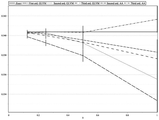 Figure 1. as functions of h: , , , .
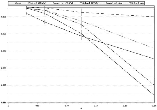 Figure 2. as functions of h: , , , .
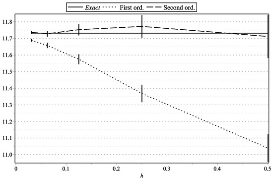 Figure 3. as functions of h: , .
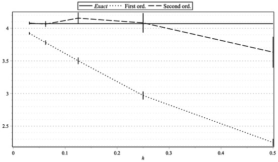 Figure 4. as functions of h: , .
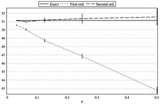 Figure 5. as functions of h: , .
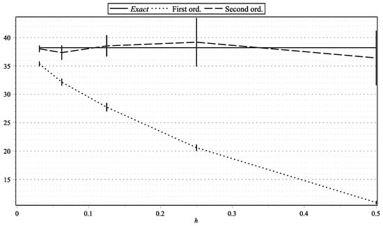 Figure 6. as functions of h: , .
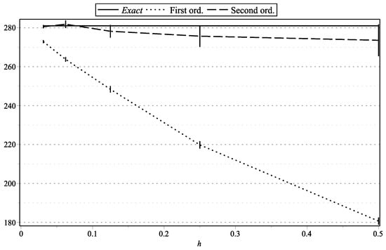 Figure 7. as functions of h: , .
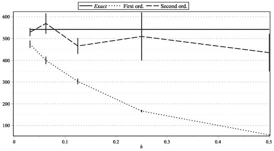 Figure 8. as functions of h: , .
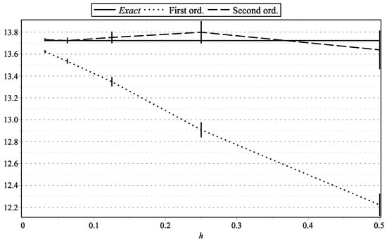 Figure 9. as functions of h: , .
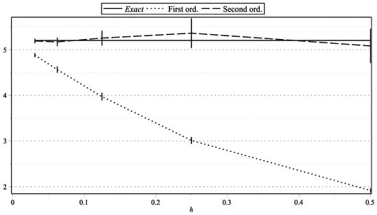 Figure 10. as functions of h: , .
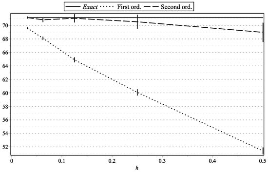 Figure 11. as functions of h: , .
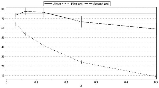 Figure 12. as functions of h: , .
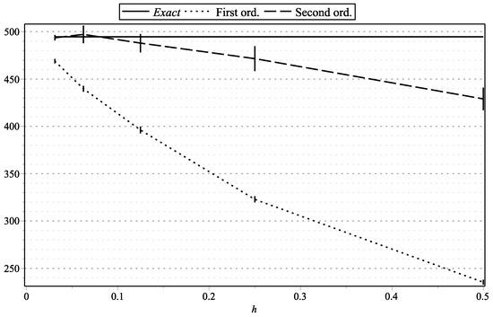 Figure 13. as functions of h: , .
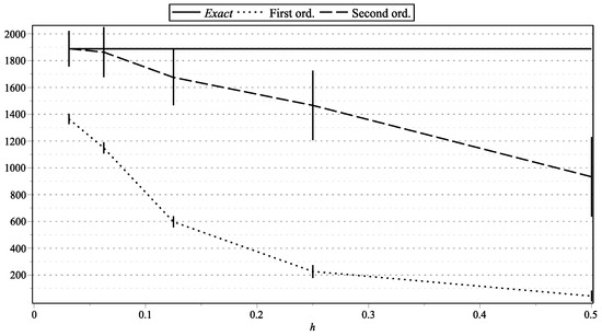 Figure 14. as functions of h: , .
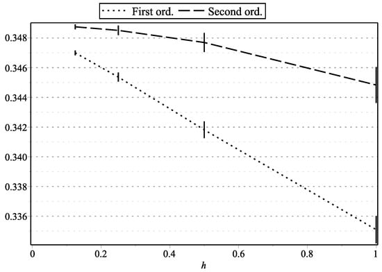 Figure 15. as functions of h: , , , .
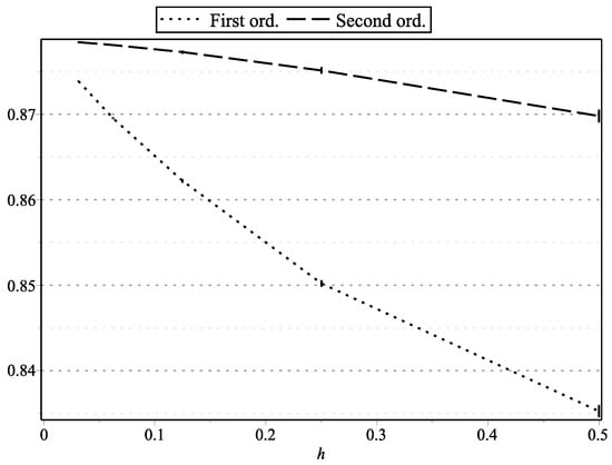 Figure 16. as functions of h: , , , .
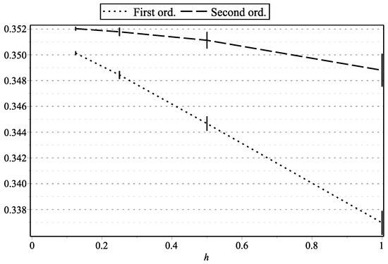 Figure 17. as functions of h: , , , .
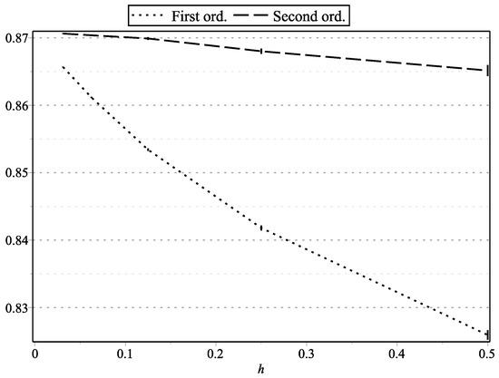 Figure 18. as functions of h: , , , .
Figure 1, Figure 15, and Figure 17 represent the values of with “low” volatility (, , , ). Figure 2, and Figure 16 and Figure 18 represent the values of with “high” volatility (, , , ). Figure 3, Figure 5, Figure 7, Figure 9, Figure 11, and Figure 13 represent values of with “low” volatility (, ). Figure 4, Figure 6, Figure 8, Figure 10, Figure 12, and Figure 14 represent the values of with “high” volatility (, ). In all the graphs, the error bars show 95% confidence intervals. To shorten the bars, for approximation time-step sizes , , we have generated samples of approximations.
In the legends of figures, we use the following notation.
- “First ord. GLVM”: the modified first-order scheme for CIR [8] [Rem. 4] (for comparison with higher-order schemes);
- “Second ord. GLVM”: our second-order scheme for CIR (Thm. 2);
- “First ord.”: our first-order scheme for CKLS [8] [Thm. 2];
- “Second ord.”: our second-order schemes for CKLS (Thm. 3);
- “Second ord. AA”: the second-order scheme of Alfonsi for CIR [5] [Thm. 2.8];
- “Third ord. AA”: the third-order scheme of Alfonsi for CIR [5] [Thm. 3.7].
7. Conclusions
We have constructed second-order weak split-step approximations of the Chan–Karolyi–Longstaff–Sanders (CKLS) and constant elasticity of variance (CEV) processes. The approximations use generation of a three−valued random variable at each discretization step. To illustrate the accuracy of constructed approximations, we performed several simulations with different parameters and test functions. Our method can be applied to constructing second-order weak approximations for other stochastic differential equations. It would be interesting to construct third-order weak approximations for the CKLS equations, as we did for the CIR equation.
Author Contributions
The authors have participated equally in the development of this work, in both the theoretical and the computational aspects. All authors have read and agreed to the published version of the manuscript.
Funding
This research received no external funding.
Institutional Review Board Statement
Not applicable.
Informed Consent Statement
Not applicable.
Data Availability Statement
Not applicable.
Conflicts of Interest
The authors declare no conflict of interest.
Abbreviations
The following abbreviations are used in this manuscript:
| CKLS | Chan–Karolyi–Longstaff–Sanders model |
| CEV | Constant elasticity of variance model |
| CIR | Cox–Ingersoll–Ross model |
| The set of positive real numbers | |
| The set of nonnegative real numbers | |
| The set of positive integers | |
| The set of nonnegative integers, | |
| The domain of the solution of CKLS, | |
| The mean of a random variable X | |
| Equidistant time interval discretization | |
| The set of infinitely differentiable functions | |
| The set of functions of class with compact support | |
| The set of functions of class with all partial derivatives of polynomial growth | |
| A function of polynomial growth with respect to , i.e., we write if for some , , and , | |
| A function of polynomial growth with respect to when the function g is expressed in terms of another function and the constants C, , and k depend on a good sequence for f only |
Appendix A
We further indicate a particular power of the stochastic part (5) by the left subscript as in . It is known (see [8] [A.7]) that
where , . Using this formula, we calculate (recall that ):
References
- Chan, K.C.; Karolyi, G.A.; Longstaff, F.A.; Sanders, A.B. An empirical investigation of alternative models of the short-term interest rate. J. Financ. 1992, 47, 1209–1227. [Google Scholar] [CrossRef]
- Cox, J.C. Notes on Option Pricing I: Constant Elasticity of Variance Diffusions, Working Paper, Stanford University, 1975. J. Portf. Manag. 1996, 23, 15–17. [Google Scholar] [CrossRef]
- Cox, J.C.; Ingersoll, J.E.; Ross, S.A. A theory of the term structure of interest rates. Econometrica 1985, 53, 385–407. [Google Scholar] [CrossRef]
- Milstein, G.N.; Tretyakov, M.V. Stochastic Numerics for Mathematical Physics; Springer: Berlin/Heidelberg, Germany, 2004. [Google Scholar]
- Alfonsi, A. High order discretization schemes for the CIR process: Application to Affine Term Structure and Heston models. Math. Comput. Am. Math. Soc. 2010, 79, 209–237. [Google Scholar] [CrossRef]
- Mackevičius, V. On approximation of CIR equation with high volatility. Math. Comput. Simul. 2010, 80, 959–970. [Google Scholar] [CrossRef]
- Mackevičius, V. Weak approximation of CIR equation by discrete random variables. Lith. Math. J. 2011, 51, 385–401. [Google Scholar] [CrossRef]
- Lileika, G.; Mackevičius, V. Weak approximation of CKLS and CEV processes by discrete random variables. Lith. Math. J. 2020, 60, 208–224. [Google Scholar] [CrossRef]
- Alfonsi, A. On the discretization schemes for the CIR (and Bessel squared) processes. Monte Carlo Methods Appl. 2005, 11, 355–384. [Google Scholar] [CrossRef]
- Mackevičius, V.; Mongirdaitė, G. On backward Kolmogorov equation related to CIR process. Mod. Stochastics Theory Appl. 2018, 5, 113–127. [Google Scholar] [CrossRef]
- Lamberton, D.; Lapeyre, B. Introduction to Stochastic Calculus Applied to Finance; Chapman & Hall: London, UK, 1996. [Google Scholar]
Publisher’s Note: MDPI stays neutral with regard to jurisdictional claims in published maps and institutional affiliations. |
© 2021 by the authors. Licensee MDPI, Basel, Switzerland. This article is an open access article distributed under the terms and conditions of the Creative Commons Attribution (CC BY) license (https://creativecommons.org/licenses/by/4.0/).