Hybrid MCDM Based on VIKOR and Cross Entropy under Rough Neutrosophic Set Theory

Abstract

Problems in real life usually involve uncertain, inconsistent and incomplete information. An example of such problems is strategic decision making with respect to remediation planning of historic pedestrian bridges. The multiple decision makers and experts, as well as the various mutually conflicting criteria, unknown criteria weights, and vagueness and duality in final decisions, provide motivation to develop a methodology that is able to resist the challenges implicit in this problem. Therefore, the aim of this research was to propose an algorithm based on the theory of rough neutrosophic sets in order to solve the problem of strategic planning with respect to the remediation of historic pedestrian bridges. A new multicriteria decision-making model is developed that is a fusion of rough set and neutrosophic set theory. A new cross entropy is proposed under a rough neutrosophic environment that does not possess the shortcomings of asymmetrical character and unknown occurrences. Additionally, a weighted rough neutrosophic symmetric cross entropy is proposed. Furthermore, a rough neutrosophic VIKOR method is introduced, with which the values of the utility measure, regret measure and VIKOR index are obtained. These values, as well as the weighted rough neutrosophic symmetric cross entropy measure, are used to provide a ranking of historic pedestrian bridges favorable to remediation. Finally, an illustrative example of the strategic planning of remediation for historic pedestrian bridges is solved and compared to other research, demonstrating the robustness, feasibility and efficacy of the model when dealing with complex multicriteria decision-making processes.

1. Introduction

Complex real-life problems are difficult to solve for a single expert, and the application of simple methods and tools in decision-making processes is insufficient when dealing with such problems. It is necessary to include a wide range of knowledge when dealing with uncertainty and vagueness in these problems. The theory of rough sets was first proposed by Pawlak [1], and has been used as a tool to process incomplete and indistinct information. The idea of rough set theory is based on lower and upper approximation in equivalence relations. It is a powerful tool in artificial intelligence applications, where it is often used in data mining and machine learning [2]. The main advantage of rough set theory, when it comes to data analysis, is that there is no need for past or supplementary information regarding the data, such as probability distribution or membership grades [2,3,4]. Different models have been proposed for various aspects of rough set theory, amalgamating it with fuzzy sets, vague sets, intuitionistic fuzzy sets, grey sets and neutrosophic sets [5].

On the other hand, neutrosophic set theory was proposed by Smarandache [6,7], and is based on three mutually independent functions: the membership function, also known as the truth function, the non-membership or falsity function, and the indeterminacy function. In this way, the vaguest and most uncertain cases can be modeled. Neutrosophic set theory is basically a generalization of fuzzy set theory, intuitionistic fuzzy sets, grey sets and vague sets based on neutrosophy [8].

Rough neutrosophic theory is a hybrid concept of rough theory and single-valued neutrosophic set theory that was introduced by Broumi [9]. Rough set theory and neutrosophic set theory are two dissimilar terms, both with the ability to deal with insufficient and uncertain information. The fusion of rough and neutrosophic theory has been shown to be useful in solving real-life problems, and usually gives better results in computational applications then any of these concepts alone [10].

Decision-making procedures are characterized by vagueness, greyness, rough reasoning, neutrosophics, and fuzziness. They evolve in response to uncertain and hybrid environments, and in order to cope with the demands of modern society, they have to be strategic and robust, rather than stagnant. Models for real-life problems are difficult to design without a thorough understanding of human decision-making processes. For this reason, it is important to involve the hybrid methodology of rough neutrosophic sets in the decision-making concept [11]. Concepts of rough neutrosophic multiattribute decision making based on grey relational analysis [12] and based on the accuracy score function [13] were developed. Mondal, Pramanik and Smarandache [14] proposed trigonometric hamming similarity measures for rough neutrosophic sets in decision making. Alias, Mohamad and Shuib [15,16] defined rough neutrosophic multiset relation properties and universally generalized the relation properties of rough fuzzy relations, rough intuitionistic fuzzy relations and rough neutrosophic relations. Pramanik et al. [17] proposed a multi-attribute strategy using bidirectional projection measures under an interval rough neutrosophic environment. Pramanik et al. [18] defined the values of the correlation coefficient between two rough neutrosophic sets. Mohana and Mohanasundari [19] studied the properties and degree of similarity between two single-valued rough neutrosophic sets. Malik, Akram and Smarandache [20] developed soft, rough neutrosophic graphs and influence cycles and trees, using them in the decision-making process, while Akram et al. [21] proposed digraphs based on the neutrosophic rough hybrid model. The concept of fuzzy equivalence on standard neutrosophic sets and rough standard neutrosophic sets was developed by Thao et al. [22]. The same concept has been applied in cluster analysis. Broumi and Smarandache [23] combined interval-valued neutrosophic soft sets and rough sets, thereby introducing the concept of interval-valued neutrosophic soft rough sets. Rough neutrosophic hyper-complex sets and the rough neutrosophic hyper-complex cosine function were developed and applied in a multiattribute decision-making approach proposed by Mondal, Pramanik and Smarandache [24].

VIKOR (VIšekriterijumsko KOmpromisno Rangiranje) [25] is a multicriteria decision-making method intended to solve decision-making problems in certain circumstances that exhibit unmeasurable and mutually conflicting criteria [26]. The method is based on ranking and selecting from a set of alternatives. It supports decision makers in reaching their final decision by defining compromise alternatives for problems with conflicting criteria. Compromise alternatives, in this case, are those solutions closest to the ideal, and are established by mutual agreement. Mardani et al. [27] made a detailed chronology of VIKOR method, from its classical to hybrid form using fuzzy techniques. Chaterjee and Chakraborty [28] analyzed the comparison of classical VIKOR method and its variant forms such as comprehensive VIKOR, fuzzy VIKOR, regret theory based VIKOR, modified and interval VIKOR. The method has been applied as multicriteria tool to various decision-making problems, such is green supply chain management [29], evaluation of service quality in airline industry [30], safety risk assessment in mine industry using Pythagorean fuzzy VIKOR-based approach [31], failure mode and effects analysis [32], evaluation of human resources managers’ competency in using VIKOR and entropy [33], integration of aggregation operators into the VIKOR for multiple criteria problems [34], extended VIKOR method for multicriteria group decision-making based on cross-entropy under the interval-valued fuzzy sets [35], VIKOR based on interval neutrosophic set environment for multicriteria decision-making problem solving [36], product design evaluation using rough sets and VIKOR [37], multicriteria group decision-making with trapezoidal neutrosophic numbers [38], industrial robot selection [39], sustainable development in EU countries using TOPSIS and VIKOR [40], and personal selection using modified fuzzy VIKOR [41]. More research on decision-making with uncertainty, inconsistency and incomplete information was given by Shekhovtsov, Kołodziejczyk and Sałabun [42], where the authors presented a study to show the difference between structured and monolith approaches when solving multicriteria decision-making problems, using the Characteristic Objects Method. Two multicriteria decision-making methods were used to obtain ranking of electric vans, the Preference Ranking Organization Method for Enrichment Evaluations (PROMETHEE) that compounds certain data, and the Technique for Order of Preference by Similarity to Ideal Solution (TOPSIS) with partially incomplete data. The fuzzy model was developed and applied in a monolithic and structured approach. Rehman et al. [43] proposed a consensus-based technique to select and evaluate suppliers under the incomplete fuzzy preference relations using $T_L$-transitivity. The defined criteria were based on the analytical hierarchy process, and alternatives were evaluated using consistent fuzzy preference relations. Faizi et al. [44] developed a new approach that combines the advantages of normalized interval-valued triangular fuzzy numbers and the Characteristic Objects Method, dealing with another source of uncertainty where the data from an expert have an error margin or are not adequately presented. Shekhovtsov and Kołodziejczyk [45] presented a study on the TOPSIS method’s accuracy that depended on the use of the normalization methods. A comparative analysis of the results was then conducted, based on the similarity coefficients of the rankings. Sałabun, Watróbski and Shekhovtsov [46] made a comparison of several multicriteria decision-making methods (TOPSIS, VIKOR, COPRAS and PROMETHEE) that are well known and mostly utilized along with similarity coefficients such as Spearman’s correlation coefficient and the WS coefficient. Faizi et al. [47] proposed two approaches of the Best-Worst method, the linear Best-Worst method and the Euclidean Best-Worst method, to obtain the priority vector of best criteria for multicriteria group decision-making problems under the intuitionist 2-tuple linguistic sets environment.

Multicriteria decision-making strategy under single-valued neutrosophic set theory was proposed by Majumdar and Samanta [48] using the entropy measure, while Ye [49] defined cross entropy for a single-valued neutrosophic set and a proposed multicriteria decision-making strategy. Pramanik et al. [50] proposed cross entropy-based multiattribute group decision-making under single-valued neutrosophic theory.

The previous studies proposed detailed methodology approaches, and applications of VIKOR and cross entropy, but none of them proposed the fusion of rough theory and neutrosophic set theory based VIKOR and cross entropy. The selection of the VIKOR method and cross entropy under the rough neutrosophic environment is justified because it uses an idea of gaining priority ranking or best choice based on reference or ideal values without triviality and exiguity in the algorithm that provides the robust outcomes of quantitative ranking of decision-making strategy. Hereby, the hybrid model of rough neutrosophic VIKOR and rough neutrosophic symmetric cross entropy is developed to strategic remediation planning of historic pedestrian bridges. Then, the comparison with other studies is provided to define similarity between rankings using $r_w$ and $WS$ coefficients [42]. The described methodology points out the motivation behind the newly developed algorithm for the strategical decision-making of historic pedestrian bridge remediation planning that involves multiple experts and mutually conflicting criteria with unknown weights. Furthermore, the main contributions of this paper are as follows:

• Definition of the rough neutrosophic symmetric cross entropy measure and proofs of its basic properties.
• Definition of the weighted rough neutrosophic symmetric cross entropy measure and proofs of its basic properties.
• Integration of rough neutrosophic theory and VIKOR method, combining it with weighted rough neutrosophic symmetric cross entropy measure.
• Development of the multicriteria decision-making strategy under rough neutrosophic set theory for historic bridges remediation planning.

The rest of the research is organized as follows: Section 2 presents the concepts of neutrosophic sets and rough neutrosophic set theory, the newly developed rough neutrosophic symmetric cross entropy measure, the basic steps of the VIKOR method and the proposed new multicriteria decision-making model. An illustrative example is presented in Section 3, demonstrating the application and efficacy of the newly proposed multicriteria decision-making strategy under rough neutrosophic theory. Section 4 gives conclusions and further research directions.

2. Materials and Methods

In this section, basic definitions of neutrosophic sets, single-valued neutrosophic sets and rough neutrosophic sets are recalled.

2.1. Neutrosophic Sets and Single-Valued Neutrosophic Sets

Definition 1 

([8]). Let $X$ be a set of objects with a generic element of $x$ denoted by $X$. A neutrosophic set $A$ in $X$ is described by a truth membership function$T_A\left(x\right)$, an indeterminacy membership function $I_A\left(x\right)$ and a falsity membership function $F_A\left(x\right)$, and is denoted as follows:

$$A=\{<x;\langle T_A\left(x\right), I_A\left(x\right), F_A\left(x\right)\rangle >|x\in X\}$$

(1)

where $T_A\left(x\right), I_A\left(x\right),$ and $F_A\left(x\right)$ are real subsets of [⁻0, 1⁺], that is $T_A\left(x\right):X\to$ [⁻0, 1⁺], $I_A\left(x\right):X\to$ [⁻0, 1⁺], and $F_A\left(x\right):X\to$ [⁻0, 1⁺]. The sum of three membership functions $T_A\left(x\right), I_A\left(x\right),$and $F_A\left(x\right)$ satisfy:

$${}^{-}0\le \sup T_A\left(x\right)+\sup I_A\left(x\right)+\sup F_A\left(x\right)\le 3^{+}$$

(2)

Definition 2 

([51]). Let $X$ be a set of objects with a generic element of $x$ denoted by $X$. A single-valued neutrosophic set $A$ in $X$ is characterized by a truth membership function$T_A\left(x\right)$, an indeterminacy membership function $I_A\left(x\right)$ and a falsity membership function $F_A\left(x\right)$, and is denoted as follows:

$$A=\left\{x,\langle T_A\left(x\right), I_A\left(x\right), F_A\left(x\right)\rangle |x\in X\right\}$$

(3)

where $T_A\left(x\right), I_A\left(x\right),$ and $F_A\left(x\right)$ $\in \left[0,1\right]$ for each x in X, and they satisfy $0\le T_A\left(x\right)+I_A\left(x\right)+F_A\left(x\right)\le 3$, and $A=\langle T_A\left(x\right), I_A\left(x\right), F_A\left(x\right)\rangle$ is known as a single-valued neutrosophic set (SVNS). The properties of SVNSs are defined as follows [52]:

• Union: The union of two SVNSs $A_1$ and $A_2$ is the neutrosophic set $A_3$ described as $A_3=A_1\cup A_2$, where $T_{A_3}\left(x\right)=max\left\{T_{A_1}\left(x\right),T_{A_2}\left(x\right)\right\}$, $I_{A_3}\left(x\right)=min\left\{I_{A_1}\left(x\right),I_{A_2}\left(x\right)\right\}$, $F_{A_3}\left(x\right)=min\left\{F_{A_1}\left(x\right),F_{A_2}\left(x\right)\right\}$.
• Intersection: The intersection of two SVNSs $A_1$ and $A_2$ is defined as $A_4=A_1\cap A_2$, where $T_{A_4}\left(x\right)=min\left\{T_{A_1}\left(x\right),T_{A_2}\left(x\right)\right\}$,$I_{A_3}\left(x\right)=max\left\{I_{A_1}\left(x\right),I_{A_2}\left(x\right)\right\}$,$F_{A_3}\left(x\right)=max\left\{F_{A_1}\left(x\right),F_{A_2}\left(x\right)\right\}$.
• Inclusion: The inclusion of two SVNSs $A_1$ and $A_2$ in $X$ is defined as $A_1\subseteq A_2$, where $T_{A_1}\left(x\right)\le T_{A_2}$, $I_{A_1}\left(x\right)\ge I_{A_2}$, $F_{A_1}\left(x\right)\ge F_{A_2}$, $\forall x\in X$.
• Equality: The equality of two SVNSs $A_1$ and $A_2$ in $X$ is defined as $A_1=A_2$, where $T_{A_1}\left(x\right)=T_{A_2}$, $I_{A_1}\left(x\right)=I_{A_2}$, $F_{A_1}\left(x\right)=F_{A_2}$, $\forall x\in X$.
• Complement: The complement of any SVNS in $X$ written as $A^c$ is defined as $A^c=\left\{x,1-T_A,1-I_A,1-F_A|x\in X\right\}$.

2.2. Rough Neutrosophic Sets

Two basic components in rough set theory, the crisp set and equivalence relation, are the mathematical basis of rough sets. The fundamental idea of a rough set is an approximation of the set known as the lower and upper approximation. Rough neutrosophic sets [5] are generalizations of rough fuzzy sets [53] and rough intuitionistic fuzzy sets [54].

Definition 3 

([52]). Let $Z$ be a non-null set and $R$ be an equivalence relation on $Z$. Let $P$ be a neutrosophic set in $Z$ with the membership function $T_P$, indeterminacy function $I_P$ and non-membership function $F_P$. The lower and the upper approximations of $A$ in the approximation $\left(Z, R\right)$ denoted by $\underset{\_}{N}\left(A\right)$ and $\overline{N}\left(A\right)$ are defined respectively as:

$$\underset{\_}{N}\left(A\right)=\langle <x, T_{\underset{\_}{N}\left(A\right)}\left(x\right),I_{\underset{\_}{N}\left(A\right)}\left(x\right), F_{\underset{\_}{N}\left(A\right)}\left(x\right)>|Z\in {\left[x\right]}_R, x\in Z\rangle$$

(4)

$$\overline{N}\left(A\right)=\langle <x, T_{\overline{N}\left(A\right)}\left(x\right),I_{\overline{N}\left(A\right)}\left(x\right), F_{\overline{N}\left(A\right)}\left(x\right)>|Z\in {\left[x\right]}_R, x\in Z\rangle$$

(5)

where $T_{\underset{\_}{N}\left(A\right)}\left(x\right)={\wedge }_z\in {\left[x\right]}_R{T}_{\left(A\right)}\left(z\right), I_{\underset{\_}{N}\left(A\right)}\left(x\right)={\wedge }_z\in {\left[x\right]}_R{I}_{\left(A\right)}\left(z\right), F_{\underset{\_}{N}\left(A\right)}\left(x\right)={\wedge }_z\in {\left[x\right]}_R{F}_{\left(A\right)}\left(z\right), T_{\overline{N}\left(A\right)}\left(x\right)={\vee }_z\in {\left[x\right]}_R{T}_{\left(A\right)}\left(z\right),$ $I_{\overline{N}\left(A\right)}\left(x\right)={\vee }_z\in {\left[x\right]}_R{I}_{\left(A\right)}\left(z\right), F_{\overline{N}\left(A\right)}\left(x\right)={\vee }_z\in {\left[x\right]}_R{F}_{\left(A\right)}\left(z\right).$ Therefore:

$$\begin{gathered} 0\le T_{\underset{\_}{N}\left(A\right)}\left(x\right)+I_{\underset{\_}{N}\left(A\right)}\left(x\right)+F_{\underset{\_}{N}\left(A\right)}\left(x\right)\le 3 \\ 0\le T_{\overline{N}\left(A\right)}\left(x\right)+I_{\overline{N}\left(A\right)}\left(x\right)+F_{\overline{N}\left(A\right)}\left(x\right)\le 3 \end{gathered}$$

(6)

Operators $\wedge$ and $\vee$ present the “min” and the “max’’, respectively. $T_{\left(A\right)}\left(z\right)$, $I_{\left(A\right)}\left(z\right)$and $F\left(z\right)$are membership, indeterminacy and non-membership of $Z$ with respect to $A$. It is obvious that $\underset{\_}{N}\left(A\right)$ and $\overline{N}\left(A\right)$ are two neutrosophic sets in $Z$. Therefore, the neutrosophic set mapping $\underset{\_}{N}$, $\overline{N}$: $N\left(Z\right) \to N\left(Z\right)$ presents the lower and upper rough neutrosophic sets approximation operators, and the pair $\left(\underset{\_}{N}\left(A\right), \overline{N}\left(A\right)\right)$ is the rough neutrosophic set in $\left(Z, R\right)$. According to Definition 3, it is obvious that $\underset{\_}{N}\left(A\right)$ and $\overline{N}\left(A\right)$ have constant membership on the equivalence clases of $R$ if $\underset{\_}{N}\left(A\right)=$ $\overline{N}\left(A\right) i.e., T_{\underset{\_}{N}\left(A\right)}\left(x\right)=T_{\overline{N}\left(A\right)}\left(x\right)$, $I_{\underset{\_}{N}\left(A\right)}\left(x\right)=I_{\overline{N}\left(A\right)}\left(x\right), F_{\underset{\_}{N}\left(A\right)}\left(x\right)=F_{\overline{N}\left(A\right)}\left(x\right).$ $A$ is a definable neutrosophic set in the approximation $\left(Z, R\right)$, and according to [55], it is easy to prove that the zero neutrosophic set $\left(0_N\right)$ and unit neutrosophic sets $\left(1_N\right)$ are definable neutrosophic sets.

If $N\left(A\right)=\left(\underset{\_}{N}\left(A\right), \overline{N}\left(A\right)\right)$ is a rough neutrosophic set in $\left(Z, R\right)$, the rough neutrosophic of $N\left(A\right)$ is a rough neutrosophic set denoted by $N\left(A\right)=\left(\underset{\_}{N}{\left(A\right)}^c,\overline{N}{\left(A\right)}^c\right)$, where $\underset{\_}{N}{\left(A\right)}^c,\overline{N}{\left(A\right)}^c$ represent the complements of neutrosophic sets of $\underset{\_}{N}\left(A\right), \overline{N}\left(A\right)$, respectively.

$$\begin{gathered} \underset{\_}{N}{\left(A\right)}^c=\langle <x, 1-T_{\underset{\_}{N}\left(A\right)}\left(x\right),1-I_{\underset{\_}{N}\left(A\right)}\left(x\right), 1-F_{\underset{\_}{N}\left(A\right)}\left(x\right)>| x\in Z\rangle \\ \overline{N}{\left(A\right)}^c=\langle <x, 1-T_{\overline{N}\left(A\right)}\left(x\right),1-I_{\overline{N}\left(A\right)}\left(x\right), 1-F_{\overline{N}\left(A\right)}\left(x\right)>| x\in Z\rangle \end{gathered}$$

(7)

If $N\left(A\right)$ and $N\left(B\right)$ are two rough neutrosophic sets in $Z$, then according to [5], the definitions are given as:

$$\begin{gathered} N\left(A\right)=N\left(B\right)\iff \underset{\_}{N}\left(A\right)=\underset{\_}{N}\left(B\right)\wedge \overline{N}\left(A\right)=\overline{N}\left(B\right) \\ N\left(A\right)\subseteq N\left(B\right)\iff \underset{\_}{N}\left(A\right)\subseteq \overline{N}\left(B\right)\wedge \overline{N}\left(A\right)\subseteq \overline{N}\left(B\right) \\ N\left(A\right)\cup N\left(B\right)\iff \underset{\_}{N}\left(A\right)\cup \underset{\_}{N}\left(B\right)\wedge \overline{N}\left(A\right)\cup \overline{N}\left(B\right) \\ N\left(A\right)\cap N\left(B\right)\iff \underset{\_}{N}\left(A\right)\cap \overline{N}\left(B\right)\wedge \overline{N}\left(A\right)\cap \overline{N}\left(B\right) \\ N\left(A\right)+N\left(B\right)\iff \underset{\_}{N}\left(A\right)+\underset{\_}{N}\left(B\right)\wedge \overline{N}\left(A\right)+\overline{N}\left(B\right) \\ N\left(A\right)\ast N\left(B\right)\iff \underset{\_}{N}\left(A\right)\ast \overline{N}\left(B\right)\wedge \overline{N}\left(A\right)\ast \overline{N}\left(B\right) \end{gathered}$$

(8)

If $A,B,C$ are rough neutrosophic sets in $\left(Z, R\right)$, then the following propositions are as follows:

Proposition 1. 

i. 

$~A\left(~A\right)=A$

ii. 

$A\cup B=A\cup B,B \cup A=A\cup B$

iii. 

$\left(C\cup B\right)\cup A=C\cup \left(B\cup A\right)$

iv. 

$\left(C\cap B\right)\cap A=C\cap \left(B\cap A\right)$

v. 

$\left(C\cup B\right)\cap A=\left(C\cup B\right)\cap \left(C\cup A\right)$

vi. 

$\left(C\cap B\right)\cap A=\left(C\cap B\right)\cap \left(C\cap A\right)$

Proposition 2. 

 

For any two neutrosophic sets, De Morgan’s laws are satisfied:

i. 

$~\left(N\left(A\right)\cup N\left(B\right)\right)=\left(~N\left(A\right)\cap N\left(B\right)\right)$

ii. 

$~\left(N\left(A\right)\cap N\left(B\right)\right)=\left(~N\left(A\right)\cup N\left(B\right)\right)$

Proposition 3.

 

If$A$and$B$are two neutrosophic sets in$U$such that$A\subseteq B$, then$N\left(A\right)\subseteq N\left(B\right)$:

i. 

$N\left(A\cap B\right)\subseteq N\left(A\right)\cap N\left(B\right)$

ii. 

$N\left(A\cup B\right)\supseteq N\left(A\right)\cup N\left(B\right)$

Proposition 4. 

 

For any rough neutrosophic set$A$:

i. 

$\underset{\_}{N}\left(A\right)=\sim \overline{N}\left(\sim A\right)$

ii. 

$\overline{N}\left(A\right)=\sim \underset{\_}{N}\left(\sim A\right)$

iii. 

$\underset{\_}{N}\left(A\right)\subseteq \overline{N}\left(A\right)$

2.3. Rough Neutrosophic Symmetric Cross Entropy Measure

In this section, a new rough neutrosophic symmetric cross entropy measure is defined to measure the difference between two rough neutrosophic variables.

Definition 4 

([56]). Let $A=\left\{a_1,a_2,\dots , a_n\right\}$ be a probability distribution on $X$, where $a_i\in \left[0, 1\right], {\displaystyle \sum }_{i=1}^n{a}_i=1$, and let $B=\left\{b_1,b_2,\dots , b_n\right\}$ be the other probability distribution on $X$, where $b_i\in \left[0, 1\right], {\displaystyle \sum }_{i=1}^n{b}_i=1$. The cross entropy between $A$ and $B$ probability distributions is described as the Kullback–Leibler distance [57], and is determined as follows:

$$CE\left(A,B\right)={\displaystyle \sum }_{i=1}^n{a}_{i}lo{g}_2\frac{a_i}{b_i}$$

(9)

which is not a distance in the formal meaning, since it does not satisfy the symmetry, i.e., $CE\left(A,B\right)\ne CE\left(B,A\right),$and the triangle inequality. Although, the symmetry can be achieved by adding $CE\left(A,B\right)$ to $CE\left(B,A\right)$, as:

$$\begin{gathered} CE\left(A,B\right)=CE\left(A,B\right)+CE\left(B,A\right) \\ CE\left(A,B\right)=alo{g}_2\frac{a}{b}+blo{g}_2\frac{b}{a} \end{gathered}$$

(10)

when $n=2$, it can be assumed that $A=\left\{a,1-a\right\}$ and $B=\left\{b,1-b\right\}$, and Equation (10) can be defined as:

$$CE\left(A,B\right)=alo{g}_2\frac{a}{b}+\left(1-a\right)lo{g}_2\frac{1-a}{1-b}+blo{g}_2\frac{b}{a}+\left(1-b\right)lo{g}_2\frac{1-b}{1-a}$$

(11)

Definition 5. 

Let$A=\left(A\left(x_1\right),A\left(x_2\right),\dots , A\left(x_n\right) \right)$and$B=\left(B\left(x_1\right),B\left(x_2\right),\dots , B\left(x_n\right) \right)$be two neutrosophic sets in the universe of discourse,$X=\left\{x_1,x_2,\dots , x_n\right\}$,$x_i\in X$. According to Equation (10), the neutrosophic symmetric cross entropy of $A\left(x_i\right)$ from $B\left(x_i\right)$ can be expressed as follows:

$$NSCE\left(A\left(x_i\right),B\left(x_i\right)\right)=A\left(x_i\right)lo{g}_2\frac{A\left(x_i\right)}{B\left(x_i\right)}+\left(1-A\left(x_i\right)\right)lo{g}_2\frac{1-A\left(x_i\right)}{1-B\left(x_i\right)}+B\left(x_i\right)lo{g}_2\frac{B\left(x_i\right)}{A\left(x_i\right)}+\left(1-B\left(x_i\right)\right)lo{g}_2\frac{1-B\left(x_i\right)}{1-A\left(x_i\right)}$$

(12)

The neutrosophic symmetric cross-entropy of $A\left(x_i\right)$ and $B\left(x_i\right)$ satisfies the following properties:

• $NSCE\left(A\left(x_i\right),B\left(x_i\right)\right)\ge 0, x_i\in X$;
• $NSCE\left(A\left(x_i\right),B\left(x_i\right)\right)=0, iff A\left(x_i\right)=B\left(x_i\right), x_i\in X$;
• $NSCE\left(A^c\left(x_i\right),B^c\left(x_i\right)\right)=NSCE\left(A\left(x_i\right),B\left(x_i\right)\right), x_i\in X$.

Definition 6. 

Let$A=\left(\underset{\_}{A},\overline{A}\right)$and$B=\left(\underset{\_}{B},\overline{B}\right)$be any two rough neutrosophic sets in$U$. Then, the rough neutrosophic symmetric cross-entropy of$A=\left(\underset{\_}{A},\overline{A}\right)=\left(\underset{\_}{T_A} , \underset{\_}{I_A} ,\underset{\_}{F_A} , \overline{T_A}, \overline{I_A}, \overline{F_A} \right)$and$B=\left(\underset{\_}{B},\overline{B}\right)=\left(\underset{\_}{T_B} , \underset{\_}{I_B} ,\underset{\_}{F_B} , \overline{T_B}, \overline{I_B}, \overline{F_B} \right)$is denoted by$RNSCE\left(A, B\right)$and defined as follows:

$$\begin{array}{ll}RNSCE\left(A\left(x_i\right),B\left(x_i\right)\right)& =\left(\underset{\_}{A}\left(x_i\right),\overline{A}\left(x_i\right)\right)lo{g}_2\frac{\left(\underset{\_}{A}\left(x_i\right),\overline{A}\left(x_i\right)\right)}{\left(\underset{\_}{B}\left(x_i\right),\overline{B}\left(x_i\right)\right)}+\left(1-\left(\underset{\_}{A}\left(x_i\right),\overline{A}\left(x_i\right)\right)\right)lo{g}_2\frac{1-\left(\underset{\_}{A}\left(x_i\right),\overline{A}\left(x_i\right)\right)}{1-\left(\underset{\_}{B}\left(x_i\right),\overline{B}\left(x_i\right)\right)}+\left(\underset{\_}{B}\left(x_i\right),\overline{B}\left(x_i\right)\right)lo{g}_2\frac{\left(\underset{\_}{B}\left(x_i\right),\overline{B}\left(x_i\right)\right)}{\left(\underset{\_}{A}\left(x_i\right),\overline{A}\left(x_i\right)\right)}+(1\\ & -\left(\underset{\_}{B}\left(x_i\right),\overline{B}\left(x_i\right)\right))lo{g}_2\frac{1-\left(\underset{\_}{B}\left(x_i\right),\overline{B}\left(x_i\right)\right)}{1-\left(\underset{\_}{A}\left(x_i\right),\overline{A}\left(x_i\right)\right)}\end{array}$$

(13)

If $B\left(x_i\right)=0$ and $A\left(x_i\right)\ne 0$, and vice versa, $RNSCE\left(A\left(x_i\right),B\left(x_i\right)\right)$ cannot be defined, and taking into the account Equation (13), the authors propose a modified rough neutrosophic symmetric cross entropy as follows:

$$\begin{array}{ll}RNSCE\left(A\left(x_i\right),B\left(x_i\right)\right)& =\left|\left(\underset{\_}{A}\left(x_i\right),\overline{A}\left(x_i\right)\right)-\left(\underset{\_}{B}\left(x_i\right),\overline{B}\left(x_i\right)\right)\right|\left|lo{g}_2\frac{\left|1-\left(\left(\underset{\_}{A}\left(x_i\right),\overline{A}\left(x_i\right)\right)-\left(\underset{\_}{B}\left(x_i\right),\overline{B}\left(x_i\right)\right)\right)\right|}{\sqrt{1+{\left|\left(\underset{\_}{A}\left(x_i\right),\overline{A}\left(x_i\right)\right)-\left(\underset{\_}{B}\left(x_i\right),\overline{B}\left(x_i\right)\right)\right|}^2}}\right|\\ & +\left|\left(1-(\underset{\_}{A}\left(x_i\right),\overline{A}\left(x_i\right)\right)\right|\left|lo{g}_2\frac{\left|1-\left(\underset{\_}{A}\left(x_i\right),\overline{A}\left(x_i\right)\right)\right|}{\sqrt{1+{\left|1-\left(\underset{\_}{B}\left(x_i\right),\overline{B}\left(x_i\right)\right)\right|}^2}}\right|\\ & +\left|\left(\underset{\_}{B}\left(x_i\right),\overline{B}\left(x_i\right)\right)-\left(\underset{\_}{A}\left(x_i\right),\overline{A}\left(x_i\right)\right)\right|\left|lo{g}_2\frac{\left|1-\left(\left(\underset{\_}{B}\left(x_i\right),\overline{B}\left(x_i\right)\right)-\left(\underset{\_}{A}\left(x_i\right),\overline{A}\left(x_i\right)\right)\right)\right|}{\sqrt{1+{\left|\left(\underset{\_}{B}\left(x_i\right),\overline{B}\left(x_i\right)\right)-\left(\underset{\_}{A}\left(x_i\right),\overline{A}\left(x_i\right)\right)\right|}^2}}\right|\\ & +\left|(1-\left(\underset{\_}{B}\left(x_i\right),\overline{B}\left(x_i\right)\right)\right|\left|lo{g}_2\frac{\left|1-\left(\underset{\_}{B}\left(x_i\right),\overline{B}\left(x_i\right)\right)\right|}{\sqrt{1+{\left|1-\left(\underset{\_}{A}\left(x_i\right),\overline{A}\left(x_i\right)\right)\right|}^2}}\right|\end{array}$$

(14)

And then:

$$\begin{array}{ll}RNSCE\left(A,B\right)=\frac{1}{n}& {\displaystyle {\displaystyle \sum }_{i=1}^n}\{\left(\underset{\_}{A}\left(x_i\right),\overline{A}\left(x_i\right)\right)-\left(\underset{\_}{B}\left(x_i\right),\overline{B}\left(x_i\right)\right)\left|lo{g}_2\frac{\left|1-\left(\left(\underset{\_}{A}\left(x_i\right),\overline{A}\left(x_i\right)\right)-\left(\underset{\_}{B}\left(x_i\right),\overline{B}\left(x_i\right)\right)\right)\right|}{\sqrt{1+{\left|\left(\underset{\_}{A}\left(x_i\right),\overline{A}\left(x_i\right)\right)-\left(\underset{\_}{B}\left(x_i\right),\overline{B}\left(x_i\right)\right)\right|}^2}}\right|\\ & +\left|\left(1-(\underset{\_}{A}\left(x_i\right),\overline{A}\left(x_i\right)\right)\right|\left|lo{g}_2\frac{\left|1-\left(\underset{\_}{A}\left(x_i\right),\overline{A}\left(x_i\right)\right)\right|}{\sqrt{1+{\left|1-\left(\underset{\_}{B}\left(x_i\right),\overline{B}\left(x_i\right)\right)\right|}^2}}\right|+\left(\underset{\_}{B}\left(x_i\right),\overline{B}\left(x_i\right)\right)\\ & -\left(\underset{\_}{A}\left(x_i\right),\overline{A}\left(x_i\right)\right)\left|lo{g}_2\frac{\left|1-\left(\left(\underset{\_}{B}\left(x_i\right),\overline{B}\left(x_i\right)\right)-\left(\underset{\_}{A}\left(x_i\right),\overline{A}\left(x_i\right)\right)\right)\right|}{\sqrt{1+{\left|\left(\underset{\_}{B}\left(x_i\right),\overline{B}\left(x_i\right)\right)-\left(\underset{\_}{A}\left(x_i\right),\overline{A}\left(x_i\right)\right)\right|}^2}}\right|\\ & +\left|(1-\left(\underset{\_}{B}\left(x_i\right),\overline{B}\left(x_i\right)\right)\right|\left|lo{g}_2\frac{\left|1-\left(\underset{\_}{B}\left(x_i\right),\overline{B}\left(x_i\right)\right)\right|}{\sqrt{1+{\left|1-\left(\underset{\_}{A}\left(x_i\right),\overline{A}\left(x_i\right)\right)\right|}^2}}\right|\}\end{array}$$

(15)

If $\left(\underset{\_}{A}\left(x_i\right),\overline{A}\left(x_i\right)\right)-\left(\underset{\_}{B}\left(x_i\right),\overline{B}\left(x_i\right)\right)\left|lo{g}_2\frac{\left|\left(\underset{\_}{A}\left(x_i\right),\overline{A}\left(x_i\right)\right)-\left(\underset{\_}{B}\left(x_i\right),\overline{B}\left(x_i\right)\right)\right|}{\sqrt{1+{\left|\left(\underset{\_}{A}\left(x_i\right),\overline{A}\left(x_i\right)\right)\right|}^2}-\sqrt{1+{\left|\left(\underset{\_}{B}\left(x_i\right),\overline{B}\left(x_i\right)\right)\right|}^2}}\right|=\left(\underset{\_}{B}\left(x_i\right),\overline{B}\left(x_i\right)\right)-\left(\underset{\_}{A}\left(x_i\right),\overline{A}\left(x_i\right)\right)\left|lo{g}_2\frac{\left|\left(\underset{\_}{B}\left(x_i\right),\overline{B}\left(x_i\right)\right)-\left(\underset{\_}{A}\left(x_i\right),\overline{A}\left(x_i\right)\right)\right|}{\sqrt{1+{\left|\left(\underset{\_}{A}\left(x_i\right),\overline{A}\left(x_i\right)\right)\right|}^2}-\sqrt{1+{\left|\left(\underset{\_}{B}\left(x_i\right),\overline{B}\left(x_i\right)\right)\right|}^2}}\right|$ then (15) can be written as:

$$\begin{array}{ll}RNSCE\left(A,B\right)=\frac{1}{n}& {\displaystyle {\displaystyle \sum }_{i=1}^n}\{2\left(\left(\underset{\_}{A}\left(x_i\right),\overline{A}\left(x_i\right)\right)-\left(\underset{\_}{B}\left(x_i\right),\overline{B}\left(x_i\right)\right)\left|lo{g}_2\frac{\left|1-\left(\left(\underset{\_}{A}\left(x_i\right),\overline{A}\left(x_i\right)\right)-\left(\underset{\_}{B}\left(x_i\right),\overline{B}\left(x_i\right)\right)\right)\right|}{\sqrt{1+{\left|\left(\underset{\_}{A}\left(x_i\right),\overline{A}\left(x_i\right)\right)-\left(\underset{\_}{B}\left(x_i\right),\overline{B}\left(x_i\right)\right)\right|}^2}}\right|\right)\\ & +\left|\left(1-(\underset{\_}{A}\left(x_i\right),\overline{A}\left(x_i\right)\right)\right|\left|lo{g}_2\frac{\left|1-\left(\underset{\_}{A}\left(x_i\right),\overline{A}\left(x_i\right)\right)\right|}{\sqrt{1+{\left|1-\left(\underset{\_}{B}\left(x_i\right),\overline{B}\left(x_i\right)\right)\right|}^2}}\right|\\ & ++\left|(1-\left(\underset{\_}{B}\left(x_i\right),\overline{B}\left(x_i\right)\right)\right|\left|lo{g}_2\frac{\left|1-\left(\underset{\_}{B}\left(x_i\right),\overline{B}\left(x_i\right)\right)\right|}{\sqrt{1+{\left|1-\left(\underset{\_}{A}\left(x_i\right),\overline{A}\left(x_i\right)\right)\right|}^2}}\right|\}\end{array}$$

(16)

Wang et al. [58] defined operational laws for two single-valued neutrosophic numbers $a_1=\langle T_1, I_1, F_1\rangle$ and $a_2=\langle T_2, I_2, F_2\rangle$ as follows:

• $a_1+$ $a_2=\langle T_1+T_2-T_1{T}_2, I_1+I_2-I_1{I}_2, F_1+F_2-F_1{F}_2\rangle$
• $a_1$ $a_2=\langle T_1{T}_2, I_1{I}_2, F_1{F}_2\rangle$
• $\lambda a_1=\langle 1-{(1-T_1)}^{\lambda },1-{(1-I_1)}^{\lambda },1-{(1-F_1)}^{\lambda }\rangle$, $\lambda \in \left[0,1\right]$.

According to [59], the sum of membership, indeterminacy and non-membership with respect to $A$ of the lower and upper rough neutrosophic sets are defined as:

• $T_A=\frac{1}{2}\left|\underset{\_}{T_A}+\overline{T_A}\right|$
• $I_A=\frac{1}{2}\left|\underset{\_}{I_A}+\overline{I_A}\right|$
• $F_A=\frac{1}{2}\left|\underset{\_}{F_A}+\overline{F_A}\right|$

Definition 7. 

Considering Wang et al.’s operational laws and Mondal et al.’s definition of relationship of lower and upper rough neutrosophic sets, the operational laws for two rough neutrosophic sets$A_1=\left(\underset{\_}{T_1} , \underset{\_}{I_1} ,\underset{\_}{F_1} , \overline{T_1}, \overline{I_1}, \overline{F_1} \right)$and$A_2=\left(\underset{\_}{T_2} , \underset{\_}{I_2} ,\underset{\_}{F_2} , \overline{T_2}, \overline{I_2}, \overline{F_2} \right)$can be written as follows:

$$A_1+A_2=\left\{\begin{array}{c}\left|\frac{1}{2}\left(\left(\underset{\_}{T_1}+\underset{\_}{T_2}\right)+\left(\overline{T_1}+\overline{T_2}\right)\right)-\frac{1}{4}\left(\underset{\_}{T_1}\underset{\_}{T_2}+\underset{\_}{T_1}\overline{T_2}+\overline{T_1}\underset{\_}{T_2}+\overline{T_1} \overline{T_2}\right)\right|,\\ \left|\frac{1}{2}\left(\left(\underset{\_}{I_1}+\underset{\_}{I_2}\right)+\left(\overline{I_1}+\overline{I_2}\right)\right)-\frac{1}{4}\left(\underset{\_}{I_1}\underset{\_}{I_2}+\underset{\_}{I_1}\overline{I_2}+\overline{I_1}\underset{\_}{I_2}+\overline{I_1} \overline{I_2}\right)\right|,\\ \left|\frac{1}{2}\left(\left(\underset{\_}{F_1}+\underset{\_}{F_2}\right)+\left(\overline{F_1}+\overline{F_2}\right)\right)-\frac{1}{4}\left(\underset{\_}{F_1}\underset{\_}{F_2}+\underset{\_}{F_1}\overline{F_2}+\overline{F_1}\underset{\_}{F_2}+\overline{F_1} \overline{F_2}\right)\right|\end{array}\right\}$$

(17)

$$A_1-A_2=\left\{\begin{array}{c}\left|\frac{1}{2}\left(\left(\underset{\_}{T_1}-\underset{\_}{T_2}\right)+\left(\overline{T_1}-\overline{T_2}\right)\right)+\frac{1}{4}\left(\underset{\_}{T_1}\underset{\_}{T_2}+\underset{\_}{T_1}\overline{T_2}+\overline{T_1}\underset{\_}{T_2}+\overline{T_1} \overline{T_2}\right)\right|,\\ \left|\frac{1}{2}\left(\left(\underset{\_}{I_1}-\underset{\_}{I_2}\right)+\left(\overline{I_1}-\overline{I_2}\right)\right)+\frac{1}{4}\left(\underset{\_}{I_1}\underset{\_}{I_2}+\underset{\_}{I_1}\overline{I_2}+\overline{I_1}\underset{\_}{I_2}+\overline{I_1} \overline{I_2}\right)\right|,\\ \left|\frac{1}{2}\left(\left(\underset{\_}{F_1}-\underset{\_}{F_2}\right)+\left(\overline{F_1}-\overline{F_2}\right)\right)+\frac{1}{4}\left(\underset{\_}{F_1}\underset{\_}{F_2}+\underset{\_}{F_1}\overline{F_2}+\overline{F_1}\underset{\_}{F_2}+\overline{F_1} \overline{F_2}\right)\right|\end{array}\right\}$$

(18)

$$A_1{A}_2=\left\{\begin{array}{c}\left|\frac{1}{4}\left(\underset{\_}{T_1}\underset{\_}{T_2}+\underset{\_}{T_1}\overline{T_2}+\overline{T_1}\underset{\_}{T_2}+\overline{T_1} \overline{T_2}\right)\right|,\left|\frac{1}{4}\left(\underset{\_}{I_1}\underset{\_}{I_2}+\underset{\_}{I_1}\overline{I_2}+\overline{I_1}\underset{\_}{I_2}+\overline{I_1} \overline{I_2}\right)\right|,\\ \left|\frac{1}{4}\left(\underset{\_}{F_1}\underset{\_}{F_2}+\underset{\_}{F_1}\overline{F_2}+\overline{F_1}\underset{\_}{F_2}+\overline{F_1} \overline{F_2}\right)\right|\end{array}\right\}$$

(19)

$$\lambda A_1=\left\{\begin{array}{c}\left|1-{\left(1-\frac{1}{2}\left(\underset{\_}{T_1}+\overline{T_1}\right)\right)}^{\lambda }\right|,\left|1-{\left(1-\frac{1}{2}\left(\underset{\_}{I_1}+\overline{I_1}\right)\right)}^{\lambda }\right|, \left|1-{\left(1-\frac{1}{2}\left(\underset{\_}{F_1}+\overline{F_1}\right)\right)}^{\lambda }\right|\end{array}\right\}$$

(20)

In the following, according to Equation (16), and Definition 7, the authors developed the rough neutrosophic symmetric cross entropy:

$$RNSCE\left(\left(\underset{\_}{A},\overline{A}\right),\left(\underset{\_}{B},\overline{B}\right)\right)=\frac{1}{2}{\displaystyle \sum }_{i=1}^n\left\{\begin{array}{c}\frac{1}{3}\left(\begin{array}{c}\left|\left(\left(\underset{\_}{T_A}\left(x_i\right)-\underset{\_}{T_B}\left(x_i\right)\right)+\left(\overline{T_A}\left(x_i\right)-\overline{T_B} \left(x_i\right)\right)\right)+\frac{1}{2}\left(\underset{\_}{T_A}\left(x_i\right)\underset{\_}{T_B}\left(x_i\right)+\underset{\_}{T_A}\left(x_i\right)\overline{T_B} \left(x_i\right)+\overline{T_A}\left(x_i\right)\underset{\_}{T_B} \left(x_i\right)+\overline{T_A}\left(x_i\right)\overline{T_B} \left(x_i\right)\right)\right|+\\ \left|\left(\left(\underset{\_}{I_A}\left(x_i\right)-\underset{\_}{I_B}\left(x_i\right)\right)+\left(\overline{I_A}\left(x_i\right)-\overline{I_B} \left(x_i\right)\right)\right)+\frac{1}{2}\left(\underset{\_}{I_A}\left(x_i\right)\underset{\_}{I_B}\left(x_i\right)+\underset{\_}{I_A}\left(x_i\right)\overline{I_B} \left(x_i\right)+\overline{I_A}\left(x_i\right)\underset{\_}{T_B} \left(x_i\right)+\overline{I_A}\left(x_i\right)\overline{I_B} \left(x_i\right)\right)\right|+\\ \left|\left(\left(\underset{\_}{F_A}\left(x_i\right)-\underset{\_}{F_B}\left(x_i\right)\right)+\left(\overline{F_A}\left(x_i\right)-\overline{F_B} \left(x_i\right)\right)\right)+\frac{1}{2}\left(\underset{\_}{F_A}\left(x_i\right)\underset{\_}{F_B}\left(x_i\right)+\underset{\_}{F_A}\left(x_i\right)\overline{F_B} \left(x_i\right)+\overline{F_A}\left(x_i\right)\underset{\_}{F_B} \left(x_i\right)+\overline{F_A}\left(x_i\right)\overline{F_B}\left(x_i\right)\right)\right|\end{array}\right)\ast \\ \left|2lo{g}_2\frac{|1-\frac{1}{6}(\begin{array}{c}\left|\left(\left(\underset{\_}{T_A}\left(x_i\right)-\underset{\_}{T_B}\left(x_i\right)\right)+\left(\overline{T_A}\left(x_i\right)-\overline{T_B} \left(x_i\right)\right)\right)+\frac{1}{2}\left(\underset{\_}{T_A}\left(x_i\right)\underset{\_}{T_B}\left(x_i\right)+\underset{\_}{T_A}\left(x_i\right)\overline{T_B} \left(x_i\right)+\overline{T_A}\left(x_i\right)\underset{\_}{T_B} \left(x_i\right)+\overline{T_A}\left(x_i\right)\overline{T_B} \left(x_i\right)\right)\right|+\\ \left|\left(\left(\underset{\_}{I_A}\left(x_i\right)-\underset{\_}{I_B}\left(x_i\right)\right)+\left(\overline{I_A}\left(x_i\right)-\overline{I_B} \left(x_i\right)\right)\right)+\frac{1}{2}\left(\underset{\_}{I_A}\left(x_i\right)\underset{\_}{I_B}\left(x_i\right)+\underset{\_}{I_A}\left(x_i\right)\overline{I_B} \left(x_i\right)+\overline{I_A}\left(x_i\right)\underset{\_}{T_B} \left(x_i\right)+\overline{I_A}\left(x_i\right)\overline{I_B} \left(x_i\right)\right)\right|+\\ \left|\left(\left(\underset{\_}{F_A}\left(x_i\right)-\underset{\_}{F_B}\left(x_i\right)\right)+\left(\overline{F_A}\left(x_i\right)-\overline{F_B} \left(x_i\right)\right)\right)+\frac{1}{2}\left(\underset{\_}{F_A}\left(x_i\right)\underset{\_}{F_B}\left(x_i\right)+\underset{\_}{F_A}\left(x_i\right)\overline{F_B} \left(x_i\right)+\overline{F_A}\left(x_i\right)\underset{\_}{F_B} \left(x_i\right)+\overline{F_A}\left(x_i\right)\overline{F_B}\left(x_i\right)\right)\right|\end{array}|}{\sqrt{1+|\frac{1}{6}\left(\begin{array}{c}\left|\left(\left(\underset{\_}{T_A}\left(x_i\right)-\underset{\_}{T_B}\left(x_i\right)\right)+\left(\overline{T_A}\left(x_i\right)-\overline{T_B} \left(x_i\right)\right)\right)+\frac{1}{2}\left(\underset{\_}{T_A}\left(x_i\right)\underset{\_}{T_B}\left(x_i\right)+\underset{\_}{T_A}\left(x_i\right)\overline{T_B} \left(x_i\right)+\overline{T_A}\left(x_i\right)\underset{\_}{T_B} \left(x_i\right)+\overline{T_A}\left(x_i\right)\overline{T_B} \left(x_i\right)\right)\right|+\\ \left|\left(\left(\underset{\_}{I_A}\left(x_i\right)-\underset{\_}{I_B}\left(x_i\right)\right)+\left(\overline{I_A}\left(x_i\right)-\overline{I_B} \left(x_i\right)\right)\right)+\frac{1}{2}\left(\underset{\_}{I_A}\left(x_i\right)\underset{\_}{I_B}\left(x_i\right)+\underset{\_}{I_A}\left(x_i\right)\overline{I_B} \left(x_i\right)+\overline{I_A}\left(x_i\right)\underset{\_}{T_B} \left(x_i\right)+\overline{I_A}\left(x_i\right)\overline{I_B} \left(x_i\right)\right)\right|+\\ \left|\left(\left(\underset{\_}{F_A}\left(x_i\right)-\underset{\_}{F_B}\left(x_i\right)\right)+\left(\overline{F_A}\left(x_i\right)-\overline{F_B} \left(x_i\right)\right)\right)+\frac{1}{2}\left(\underset{\_}{F_A}\left(x_i\right)\underset{\_}{F_B}\left(x_i\right)+\underset{\_}{F_A}\left(x_i\right)\overline{F_B} \left(x_i\right)+\overline{F_A}\left(x_i\right)\underset{\_}{F_B} \left(x_i\right)+\overline{F_A}\left(x_i\right)\overline{F_B}\left(x_i\right)\right)\right|\end{array}\right){|}^2}}\right|+\\ \left|6-\frac{1}{6}\left(\underset{\_}{T_A}\left(x_i\right)+\overline{T_A}\left(x_i\right)+\underset{\_}{I_A}\left(x_i\right)+\overline{I_A}\left(x_i\right)+\underset{\_}{F_A}\left(x_i\right)+\overline{F_A}\left(x_i\right)\right)\right|\ast \\ \left|lo{g}_2\left(\frac{\left|6-\frac{1}{6}\left(\underset{\_}{T_A}\left(x_i\right)+\overline{T_A}\left(x_i\right)+\underset{\_}{I_A}\left(x_i\right)+\overline{I_A}\left(x_i\right)+\underset{\_}{F_A}\left(x_i\right)+\overline{F_A}\left(x_i\right)\right)\right|}{\sqrt{1+{\left|6-\frac{1}{6}\left(\underset{\_}{T_B}\left(x_i\right)+\overline{T_B}\left(x_i\right)+\underset{\underset{·}{\_}}{I_B}\left(x_i\right)+\overline{I_B}\left(x_i\right)+\underset{\_}{F_B}\left(x_i\right)+\overline{F_B}\left(x_i\right)\right)\right|}^2}}\right)\right|+\\ \left|6-\frac{1}{6}\left(\underset{\_}{T_B}\left(x_i\right)+\overline{T_B}\left(x_i\right)+\underset{\_}{I_B}\left(x_i\right)+\overline{I_B}\left(x_i\right)+\underset{\_}{F_B}\left(x_i\right)+\overline{F_B}\left(x_i\right)\right)\right|\ast \\ \left|lo{g}_2\left(\frac{\left|6-\frac{1}{6}\left(\underset{\_}{T_B}\left(x_i\right)+\overline{T_B}\left(x_i\right)+\underset{\_}{I_B}\left(x_i\right)+\overline{I_B}\left(x_i\right)+\underset{\_}{F_B}\left(x_i\right)+\overline{F_B}\left(x_i\right)\right)\right|}{\sqrt{1+{\left|6-\frac{1}{6}\left(\underset{\_}{T_A}\left(x_i\right)+\overline{T_A}\left(x_i\right)+\underset{\_}{I_A}\left(x_i\right)+\overline{I_A}\left(x_i\right)+\underset{\_}{F_A}\left(x_i\right)+\overline{F_A}\left(x_i\right)\right)\right|}^2}}\right)\right|\end{array}\right\}$$

(21)

Example 1. 

Let A and B be two rough neutrosophic sets in Z, given by$A=$ $\langle x, \left(0.2, 0.3, 0.4\right),\left(0.4, 0.3, 0.2\right)|x\in X\rangle$and$B=\langle x, \left(0.3, 0.4, 0.5\right),\left(0.5, 0.4, 0.4\right)|x\in X\rangle$. Using (21), the rough neutrosophic symmetric cross entropy of value A and B is obtained as$RNSCE\left(\left(\underset{\_}{A},\overline{A}\right),\left(\underset{\_}{B},\overline{B}\right)\right)=0.28$.

Theorem 1. 

Rough neutrosophic symmetric cross entropy$RNSCE\left(A,B\right)$for any two rough neutrosophic sets A, B satisfies the following properties:

• $RNSCE\left(\left(\underset{\_}{A},\overline{A}\right),\left(\underset{\_}{B},\overline{B}\right)\right)\ge 0$
• $RNSCE\left(\left(\underset{\_}{A},\overline{A}\right),\left(\underset{\_}{B},\overline{B}\right)\right)=0$ iff $T_{\underset{\_}{A}}\left(x_i\right)=T_{\underset{\_}{B}}\left(x_i\right)$, $T_{\overline{A}}\left(x_i\right)=T_{\overline{B}}\left(x_i\right),$ $I_{\underset{\_}{A}}\left(x_i\right)=I_{\underset{\_}{B}}\left(x_i\right),I_{\overline{A}}\left(x_i\right)=I_{\overline{B}}\left(x_i\right),$ $F_{\underset{\_}{A}}\left(x_i\right)=F_{\underset{\_}{B}}\left(x_i\right)$, $F_{\overline{A}}\left(x_i\right)=F_{\overline{B}}\left(x_i\right),$ $\forall x_{i }\in X$
• $RNSCE\left(\left(\underset{\_}{A},\overline{A}\right),\left(\underset{\_}{B},\overline{B}\right)\right)=RNSCE\left(\left(\underset{\_}{B},\overline{B}\right), \left(\underset{\_}{A},\overline{A}\right)\right)$

Proof. 

(i) For all values of $x_i\in X$, $T_{\underset{\_}{A}}\left(x_i\right)\ge 0,T_{\overline{A}}\left(x_i\right)\ge 0, T_{\underset{\_}{B}}\left(x_i\right)\ge 0, T_{\overline{B}}\left(x_i\right)\ge 0,$

$$\left[\left|\left(\left(T_{\underset{\_}{A}}\left(x_i\right)-T_{\underset{\_}{B}}\left(x_i\right)\right)+\left(T_{\overline{A}}\left(x_i\right)-T_{\overline{B}}\left(x_i\right)\right)\right)+\frac{1}{2}\left(T_{\underset{\_}{A}}\left(x_i\right)T_{\underset{\_}{B}}\left(x_i\right)+T_{\overline{A}}\left(x_i\right)T_{\overline{B}} \left(x_i\right)+T_{\overline{A}}\left(x_i\right)T_{\overline{B}} \left(x_i\right)+T_{\overline{A}}\left(x_i\right)T_{\overline{B}}\left(x_i\right)\right)\right|\right]\ge 0.$$

Similarly, $I_{\underset{\_}{A}}\left(x_i\right)\ge 0,I_{\overline{A}}\left(x_i\right)\ge 0, I_{\underset{\_}{B}}\left(x_i\right)\ge 0, I_{\overline{B}}\left(x_i\right)\ge 0,$

$$\begin{array}{c}\left[\left|\left(\left(I_{\underset{\_}{A}}\left(x_i\right)-I_{\underset{\_}{B}}\left(x_i\right)\right)+\left(I_{\overline{A}}\left(x_i\right)-I_{\overline{B}}\left(x_i\right)\right)\right)+\frac{1}{2}\left(I_{\underset{\_}{A}}\left(x_i\right)I_{\underset{\_}{B}}\left(x_i\right)+I_{\overline{A}}\left(x_i\right)I_{\overline{B}} \left(x_i\right)+I_{\overline{A}}\left(x_i\right)I_{\overline{B}} \left(x_i\right)+I_{\overline{A}}\left(x_i\right)I_{\overline{B}}\left(x_i\right)\right)\right|\right]\ge 0\end{array},$$

and

$$\left[\left|\left(\left(T_{\underset{\_}{A}}\left(x_i\right)-T_{\underset{\_}{B}}\left(x_i\right)\right)+\left(T_{\overline{A}}\left(x_i\right)-T_{\overline{B}}\left(x_i\right)\right)\right)+\frac{1}{2}\left(T_{\underset{\_}{A}}\left(x_i\right)T_{\underset{\_}{B}}\left(x_i\right)+T_{\overline{A}}\left(x_i\right)T_{\overline{B}} \left(x_i\right)+T_{\overline{A}}\left(x_i\right)T_{\overline{B}} \left(x_i\right)+T_{\overline{A}}\left(x_i\right)T_{\overline{B}}\left(x_i\right)\right)\right|\right]\ge 0.$$

Then

$$\begin{gathered} \left[\right|2lo{g}_2\frac{|1-\frac{1}{6}(\begin{array}{c}\left|\left(\left(\underset{\_}{T_A}\left(x_i\right)-\underset{\_}{T_B}\left(x_i\right)\right)+\left(\overline{T_A}\left(x_i\right)-\overline{T_B} \left(x_i\right)\right)\right)+\frac{1}{2}\left(\underset{\_}{T_A}\left(x_i\right)\underset{\_}{T_B}\left(x_i\right)+\underset{\_}{T_A}\left(x_i\right)\overline{T_B} \left(x_i\right)+\overline{T_A}\left(x_i\right)\underset{\_}{T_B} \left(x_i\right)+\overline{T_A}\left(x_i\right)\overline{T_B} \left(x_i\right)\right)\right|+\\ \left|\left(\left(\underset{\_}{I_A}\left(x_i\right)-\underset{\_}{I_B}\left(x_i\right)\right)+\left(\overline{I_A}\left(x_i\right)-\overline{I_B} \left(x_i\right)\right)\right)+\frac{1}{2}\left(\underset{\_}{I_A}\left(x_i\right)\underset{\_}{I_B}\left(x_i\right)+\underset{\_}{I_A}\left(x_i\right)\overline{I_B} \left(x_i\right)+\overline{I_A}\left(x_i\right)\underset{\_}{T_B} \left(x_i\right)+\overline{I_A}\left(x_i\right)\overline{I_B} \left(x_i\right)\right)\right|+\\ \left|\left(\left(\underset{\_}{F_A}\left(x_i\right)-\underset{\_}{F_B}\left(x_i\right)\right)+\left(\overline{F_A}\left(x_i\right)-\overline{F_B} \left(x_i\right)\right)\right)+\frac{1}{2}\left(\underset{\_}{F_A}\left(x_i\right)\underset{\_}{F_B}\left(x_i\right)+\underset{\_}{F_A}\left(x_i\right)\overline{F_B} \left(x_i\right)+\overline{F_A}\left(x_i\right)\underset{\_}{F_B} \left(x_i\right)+\overline{F_A}\left(x_i\right)\overline{F_B}\left(x_i\right)\right)\right|\end{array}|}{\sqrt{1+|\frac{1}{6}\left(\begin{array}{c}\left|\left(\left(\underset{\_}{T_A}\left(x_i\right)-\underset{\_}{T_B}\left(x_i\right)\right)+\left(\overline{T_A}\left(x_i\right)-\overline{T_B} \left(x_i\right)\right)\right)+\frac{1}{2}\left(\underset{\_}{T_A}\left(x_i\right)\underset{\_}{T_B}\left(x_i\right)+\underset{\_}{T_A}\left(x_i\right)\overline{T_B} \left(x_i\right)+\overline{T_A}\left(x_i\right)\underset{\_}{T_B} \left(x_i\right)+\overline{T_A}\left(x_i\right)\overline{T_B} \left(x_i\right)\right)\right|+\\ \left|\left(\left(\underset{\_}{I_A}\left(x_i\right)-\underset{\_}{I_B}\left(x_i\right)\right)+\left(\overline{I_A}\left(x_i\right)-\overline{I_B} \left(x_i\right)\right)\right)+\frac{1}{2}\left(\underset{\_}{I_A}\left(x_i\right)\underset{\_}{I_B}\left(x_i\right)+\underset{\_}{I_A}\left(x_i\right)\overline{I_B} \left(x_i\right)+\overline{I_A}\left(x_i\right)\underset{\_}{T_B} \left(x_i\right)+\overline{I_A}\left(x_i\right)\overline{I_B} \left(x_i\right)\right)\right|+\\ \left|\left(\left(\underset{\_}{F_A}\left(x_i\right)-\underset{\_}{F_B}\left(x_i\right)\right)+\left(\overline{F_A}\left(x_i\right)-\overline{F_B} \left(x_i\right)\right)\right)+\frac{1}{2}\left(\underset{\_}{F_A}\left(x_i\right)\underset{\_}{F_B}\left(x_i\right)+\underset{\_}{F_A}\left(x_i\right)\overline{F_B} \left(x_i\right)+\overline{F_A}\left(x_i\right)\underset{\_}{F_B} \left(x_i\right)+\overline{F_A}\left(x_i\right)\overline{F_B}\left(x_i\right)\right)\right|\end{array}\right){|}^2}}\left|\right]\ge 0, \\ \left[\left|6-\frac{1}{6}\left(\underset{\_}{T_A}\left(x_i\right)+\overline{T_A}\left(x_i\right)+\underset{\_}{I_A}\left(x_i\right)+\overline{I_A}\left(x_i\right)+\underset{\_}{F_A}\left(x_i\right)+\overline{F_A}\left(x_i\right)\right)\right|\right]\ge 0, \\ \left[\left|6-\frac{1}{6}\left(\underset{\_}{T_B}\left(x_i\right)+\overline{T_B}\left(x_i\right)+\underset{\_}{I_B}\left(x_i\right)+\overline{I_B}\left(x_i\right)+\underset{\_}{F_B}\left(x_i\right)+\overline{F_B}\left(x_i\right)\right)\right|\right]\ge 0, \\ \left[\right|lo{g}_2\left(\frac{\left|6-\frac{1}{6}\left(\underset{\_}{T_A}\left(x_i\right)+\overline{T_A}\left(x_i\right)+\underset{\_}{I_A}\left(x_i\right)+\overline{I_A}\left(x_i\right)+\underset{\_}{F_A}\left(x_i\right)+\overline{F_A}\left(x_i\right)\right)\right|}{\sqrt{1+{\left|6-\frac{1}{6}\left(\underset{\_}{T_B}\left(x_i\right)+\overline{T_B}\left(x_i\right)+\underset{\underset{·}{\_}}{I_B}\left(x_i\right)+\overline{I_B}\left(x_i\right)+\underset{\_}{F_B}\left(x_i\right)+\overline{F_B}\left(x_i\right)\right)\right|}^2}}\right)\left|\right]\ge 0, \end{gathered}$$

and

$$\left[\right|lo{g}_2\left(\frac{\left|6-\frac{1}{6}\left(\underset{\_}{T_B}\left(x_i\right)+\overline{T_B}\left(x_i\right)+\underset{\_}{I_B}\left(x_i\right)+\overline{I_B}\left(x_i\right)+\underset{\_}{F_B}\left(x_i\right)+\overline{F_B}\left(x_i\right)\right)\right|}{\sqrt{1+{\left|6-\frac{1}{6}\left(\underset{\_}{T_A}\left(x_i\right)+\overline{T_A}\left(x_i\right)+\underset{\_}{I_A}\left(x_i\right)+\overline{I_A}\left(x_i\right)+\underset{\_}{F_A}\left(x_i\right)+\overline{F_A}\left(x_i\right)\right)\right|}^2}}\right)\left|\right]\ge 0.$$

Therefore, $RNSCE\left(\left(\underset{\_}{A},\overline{A}\right),\left(\underset{\_}{B},\overline{B}\right)\right)\ge 0,$ and it completes the proof.

(ii)

$$\begin{array}{l}\left[\begin{array}{c}\frac{1}{3}\left(\begin{array}{c}\left|\left(\left(\underset{\_}{T_A}\left(x_i\right)-\underset{\_}{T_B}\left(x_i\right)\right)+\left(\overline{T_A}\left(x_i\right)-\overline{T_B} \left(x_i\right)\right)\right)+\frac{1}{2}\left(\underset{\_}{T_A}\left(x_i\right)\underset{\_}{T_B}\left(x_i\right)+\underset{\_}{T_A}\left(x_i\right)\overline{T_B} \left(x_i\right)+\overline{T_A}\left(x_i\right)\underset{\_}{T_B} \left(x_i\right)+\overline{T_A}\left(x_i\right)\overline{T_B} \left(x_i\right)\right)\right|+\\ \left|\left(\left(\underset{\_}{I_A}\left(x_i\right)-\underset{\_}{I_B}\left(x_i\right)\right)+\left(\overline{I_A}\left(x_i\right)-\overline{I_B} \left(x_i\right)\right)\right)+\frac{1}{2}\left(\underset{\_}{I_A}\left(x_i\right)\underset{\_}{I_B}\left(x_i\right)+\underset{\_}{I_A}\left(x_i\right)\overline{I_B} \left(x_i\right)+\overline{I_A}\left(x_i\right)\underset{\_}{T_B} \left(x_i\right)+\overline{I_A}\left(x_i\right)\overline{I_B} \left(x_i\right)\right)\right|+\\ \left|\left(\left(\underset{\_}{F_A}\left(x_i\right)-\underset{\_}{F_B}\left(x_i\right)\right)+\left(\overline{F_A}\left(x_i\right)-\overline{F_B} \left(x_i\right)\right)\right)+\frac{1}{2}\left(\underset{\_}{F_A}\left(x_i\right)\underset{\_}{F_B}\left(x_i\right)+\underset{\_}{F_A}\left(x_i\right)\overline{F_B} \left(x_i\right)+\overline{F_A}\left(x_i\right)\underset{\_}{F_B} \left(x_i\right)+\overline{F_A}\left(x_i\right)\overline{F_B}\left(x_i\right)\right)\right|\end{array}\right)\times \\ \left|2lo{g}_2\frac{|1-\frac{1}{6}(\begin{array}{c}\left|\left(\left(\underset{\_}{T_A}\left(x_i\right)-\underset{\_}{T_B}\left(x_i\right)\right)+\left(\overline{T_A}\left(x_i\right)-\overline{T_B} \left(x_i\right)\right)\right)+\frac{1}{2}\left(\underset{\_}{T_A}\left(x_i\right)\underset{\_}{T_B}\left(x_i\right)+\underset{\_}{T_A}\left(x_i\right)\overline{T_B} \left(x_i\right)+\overline{T_A}\left(x_i\right)\underset{\_}{T_B} \left(x_i\right)+\overline{T_A}\left(x_i\right)\overline{T_B} \left(x_i\right)\right)\right|+\\ \left|\left(\left(\underset{\_}{I_A}\left(x_i\right)-\underset{\_}{I_B}\left(x_i\right)\right)+\left(\overline{I_A}\left(x_i\right)-\overline{I_B} \left(x_i\right)\right)\right)+\frac{1}{2}\left(\underset{\_}{I_A}\left(x_i\right)\underset{\_}{I_B}\left(x_i\right)+\underset{\_}{I_A}\left(x_i\right)\overline{I_B} \left(x_i\right)+\overline{I_A}\left(x_i\right)\underset{\_}{T_B} \left(x_i\right)+\overline{I_A}\left(x_i\right)\overline{I_B} \left(x_i\right)\right)\right|+\\ \left|\left(\left(\underset{\_}{F_A}\left(x_i\right)-\underset{\_}{F_B}\left(x_i\right)\right)+\left(\overline{F_A}\left(x_i\right)-\overline{F_B} \left(x_i\right)\right)\right)+\frac{1}{2}\left(\underset{\_}{F_A}\left(x_i\right)\underset{\_}{F_B}\left(x_i\right)+\underset{\_}{F_A}\left(x_i\right)\overline{F_B} \left(x_i\right)+\overline{F_A}\left(x_i\right)\underset{\_}{F_B} \left(x_i\right)+\overline{F_A}\left(x_i\right)\overline{F_B}\left(x_i\right)\right)\right|\end{array}|}{\sqrt{1+|\frac{1}{6}\left(\begin{array}{c}\left|\left(\left(\underset{\_}{T_A}\left(x_i\right)-\underset{\_}{T_B}\left(x_i\right)\right)+\left(\overline{T_A}\left(x_i\right)-\overline{T_B} \left(x_i\right)\right)\right)+\frac{1}{2}\left(\underset{\_}{T_A}\left(x_i\right)\underset{\_}{T_B}\left(x_i\right)+\underset{\_}{T_A}\left(x_i\right)\overline{T_B} \left(x_i\right)+\overline{T_A}\left(x_i\right)\underset{\_}{T_B} \left(x_i\right)+\overline{T_A}\left(x_i\right)\overline{T_B} \left(x_i\right)\right)\right|+\\ \left|\left(\left(\underset{\_}{I_A}\left(x_i\right)-\underset{\_}{I_B}\left(x_i\right)\right)+\left(\overline{I_A}\left(x_i\right)-\overline{I_B} \left(x_i\right)\right)\right)+\frac{1}{2}\left(\underset{\_}{I_A}\left(x_i\right)\underset{\_}{I_B}\left(x_i\right)+\underset{\_}{I_A}\left(x_i\right)\overline{I_B} \left(x_i\right)+\overline{I_A}\left(x_i\right)\underset{\_}{T_B} \left(x_i\right)+\overline{I_A}\left(x_i\right)\overline{I_B} \left(x_i\right)\right)\right|+\\ \left|\left(\left(\underset{\_}{F_A}\left(x_i\right)-\underset{\_}{F_B}\left(x_i\right)\right)+\left(\overline{F_A}\left(x_i\right)-\overline{F_B} \left(x_i\right)\right)\right)+\frac{1}{2}\left(\underset{\_}{F_A}\left(x_i\right)\underset{\_}{F_B}\left(x_i\right)+\underset{\_}{F_A}\left(x_i\right)\overline{F_B} \left(x_i\right)+\overline{F_A}\left(x_i\right)\underset{\_}{F_B} \left(x_i\right)+\overline{F_A}\left(x_i\right)\overline{F_B}\left(x_i\right)\right)\right|\end{array}\right){|}^2}}\right|\end{array}\right]=0\\ \iff T_{\underset{\_}{A}}\left(x_i\right)=T_{\underset{\_}{B}}\left(x_i\right),T_{\overline{A}}\left(x_i\right)=T_{\overline{B}}\left(x_i\right), I_{\underset{\_}{A}}\left(x_i\right)=I_{\underset{\_}{B}}\left(x_i\right),I_{\overline{A}}\left(x_i\right)=I_{\overline{B}}\left(x_i\right),F_{\underset{\_}{A}}\left(x_i\right)=F_{\underset{\_}{B}}\left(x_i\right),F_{\overline{A}}\left(x_i\right)=F_{\overline{B}}\left(x_i\right).\\ \begin{array}{c}\left[\right|6-\frac{1}{6}\left(\underset{\_}{T_A}\left(x_i\right)+\overline{T_A}\left(x_i\right)+\underset{\_}{I_A}\left(x_i\right)+\overline{I_A}\left(x_i\right)+\underset{\_}{F_A}\left(x_i\right)+\overline{F_A}\left(x_i\right)\right)|\hfill \\ \times \left|lo{g}_2\left(\frac{\left|6-\frac{1}{6}\left(\underset{\_}{T_A}\left(x_i\right)+\overline{T_A}\left(x_i\right)+\underset{\_}{I_A}\left(x_i\right)+\overline{I_A}\left(x_i\right)+\underset{\_}{F_A}\left(x_i\right)+\overline{F_A}\left(x_i\right)\right)\right|}{\sqrt{1+{\left|6-\frac{1}{6}\left(\underset{\_}{T_B}\left(x_i\right)+\overline{T_B}\left(x_i\right)+\underset{\underset{·}{\_}}{I_B}\left(x_i\right)+\overline{I_B}\left(x_i\right)+\underset{\_}{F_B}\left(x_i\right)+\overline{F_B}\left(x_i\right)\right)\right|}^2}}\right)\right|]=0\iff T_{\underset{\_}{A}}\left(x_i\right)\\ =T_{\underset{\_}{B}}\left(x_i\right),T_{\overline{A}}\left(x_i\right)=T_{\overline{B}}\left(x_i\right), I_{\underset{\_}{A}}\left(x_i\right)=I_{\underset{\_}{B}}\left(x_i\right),I_{\overline{A}}\left(x_i\right)=I_{\overline{B}}\left(x_i\right),F_{\underset{\_}{A}}\left(x_i\right)=F_{\underset{\_}{B}}\left(x_i\right),F_{\overline{A}}\left(x_i\right)=F_{\overline{B}}\left(x_i\right).\end{array}\\ \begin{array}{c} \left[\right|6-\frac{1}{6}\left(\underset{\_}{T_B}\left(x_i\right)+\overline{T_B}\left(x_i\right)+\underset{\_}{I_B}\left(x_i\right)+\overline{I_B}\left(x_i\right)+\underset{\_}{F_B}\left(x_i\right)+\overline{F_B}\left(x_i\right)\right)|\\ \times \left|lo{g}_2\left(\frac{\left|6-\frac{1}{6}\left(\underset{\_}{T_B}\left(x_i\right)+\overline{T_B}\left(x_i\right)+\underset{\_}{I_B}\left(x_i\right)+\overline{I_B}\left(x_i\right)+\underset{\_}{F_B}\left(x_i\right)+\overline{F_B}\left(x_i\right)\right)\right|}{\sqrt{1+{\left|6-\frac{1}{6}\left(\underset{\_}{T_A}\left(x_i\right)+\overline{T_A}\left(x_i\right)+\underset{\_}{I_A}\left(x_i\right)+\overline{I_A}\left(x_i\right)+\underset{\_}{F_A}\left(x_i\right)+\overline{F_A}\left(x_i\right)\right)\right|}^2}}\right)\right|]=0\end{array}\\ \iff T_{\underset{\_}{A}}\left(x_i\right)=T_{\underset{\_}{B}}\left(x_i\right),T_{\overline{A}}\left(x_i\right)=T_{\overline{B}}\left(x_i\right), I_{\underset{\_}{A}}\left(x_i\right)=I_{\underset{\_}{B}}\left(x_i\right),I_{\overline{A}}\left(x_i\right)=I_{\overline{B}}\left(x_i\right),F_{\underset{\_}{A}}\left(x_i\right)=F_{\underset{\_}{B}}\left(x_i\right),F_{\overline{A}}\left(x_i\right)=F_{\overline{B}}\left(x_i\right).\end{array}$$

Therefore, $RNSCE\left(\left(\underset{\_}{A},\overline{A}\right),\left(\underset{\_}{B},\overline{B}\right)\right)=0 \mathrm{iff} T_{\underset{\_}{A}}\left(x_i\right)=T_{\underset{\_}{B}}\left(x_i\right), T_{\overline{A}}\left(x_i\right)=T_{\overline{B}}\left(x_i\right), I_{\underset{\_}{A}}\left(x_i\right)=$

$I_{\underset{\_}{B}}\left(x_i\right),I_{\overline{A}}\left(x_i\right)=I_{\overline{B}}\left(x_i\right), F_{\underset{\_}{A}}\left(x_i\right)=F_{\underset{\_}{B}}\left(x_i\right), F_{\overline{A}}\left(x_i\right)=F_{\overline{B}}\left(x_i\right), \forall x_{i }\in X$. Hence, the proof is completed.

(iii) As is, $\left[\left|\left(\left(T_{\underset{\_}{A}}\left(x_i\right)-T_{\underset{\_}{B}}\left(x_i\right)\right)+\left(T_{\overline{A}}\left(x_i\right)- T_{\overline{B}}\left(x_i\right)\right)\right)+\frac{1}{2}\left(T_{\underset{\_}{A}}\left(x_i\right)T_{\underset{\_}{B}}\left(x_i\right)+T_{\overline{A}}\left(x_i\right)T_{\overline{B}} \left(x_i\right)+T_{\overline{A}}\left(x_i\right)T_{\overline{B}} \left(x_i\right)+T_{\overline{A}}\left(x_i\right)T_{\overline{B}}\left(x_i\right)\right)\right|\right]$

$=\left[\left|\left(\left(T_{\underset{\_}{B}}\left(x_i\right)-T_{\underset{\_}{A}}\left(x_i\right)\right)+\left(T_{\overline{B}}\left(x_i\right)- T_{\overline{A}}\left(x_i\right)\right)\right)+\frac{1}{2}\left(T_{\underset{\_}{B}}\left(x_i\right)T_{\underset{\_}{A}}\left(x_i\right)+T_{\overline{B}}\left(x_i\right)T_{\overline{A}} \left(x_i\right)+T_{\overline{B}}\left(x_i\right)T_{\overline{A}} \left(x_i\right)+T_{\overline{B}}\left(x_i\right)T_{\overline{A}}\left(x_i\right)\right)\right|\right],$

$\left[\left|\left(\left(I_{\underset{\_}{A}}\left(x_i\right)-I_{\underset{\_}{B}}\left(x_i\right)\right)+\left(I_{\overline{A}}\left(x_i\right)- I_{\overline{B}}\left(x_i\right)\right)\right)+\frac{1}{2}\left(I_{\underset{\_}{A}}\left(x_i\right)I_{\underset{\_}{B}}\left(x_i\right)+I_{\overline{A}}\left(x_i\right)I_{\overline{B}} \left(x_i\right)+I_{\overline{A}}\left(x_i\right)I_{\overline{B}} \left(x_i\right)+I_{\overline{A}}\left(x_i\right)I_{\overline{B}}\left(x_i\right)\right)\right|\right]=$

$\left[\left|\left(\left(I_{\underset{\_}{B}}\left(x_i\right)-I_{\underset{\_}{A}}\left(x_i\right)\right)+\left(I_{\overline{B}}\left(x_i\right)- I_{\overline{A}}\left(x_i\right)\right)\right)+\frac{1}{2}\left(I_{\underset{\_}{B}}\left(x_i\right)I_{\underset{\_}{A}}\left(x_i\right)+I_{\overline{B}}\left(x_i\right)I_{\overline{A}} \left(x_i\right)+I_{\overline{B}}\left(x_i\right)I_{\overline{A}} \left(x_i\right)+I_{\overline{B}}\left(x_i\right)I_{\overline{A}}\left(x_i\right)\right)\right|\right],$

$\left[\left|\left(\left(F_{\underset{\_}{A}}\left(x_i\right)-F_{\underset{\_}{B}}\left(x_i\right)\right)+\left(F_{\overline{A}}\left(x_i\right)- F_{\overline{B}}\left(x_i\right)\right)\right)+\frac{1}{2}\left(F_{\underset{\_}{A}}\left(x_i\right)F_{\underset{\_}{B}}\left(x_i\right)+F_{\overline{A}}\left(x_i\right)F_{\overline{B}} \left(x_i\right)+F_{\overline{A}}\left(x_i\right)F_{\overline{B}} \left(x_i\right)+F_{\overline{A}}\left(x_i\right)F_{\overline{B}}\left(x_i\right)\right)\right|\right]=$

$\left[\left|\left(\left(F_{\underset{\_}{B}}\left(x_i\right)-F_{\underset{\_}{A}}\left(x_i\right)\right)+\left(F_{\overline{B}}\left(x_i\right)- F_{\overline{A}}\left(x_i\right)\right)\right)+\frac{1}{2}\left(F_{\underset{\_}{B}}\left(x_i\right)F_{\underset{\_}{A}}\left(x_i\right)+F_{\overline{B}}\left(x_i\right)F_{\overline{A}} \left(x_i\right)+F_{\overline{B}}\left(x_i\right)F_{\overline{A}} \left(x_i\right)+F_{\overline{B}}\left(x_i\right)F_{\overline{A}}\left(x_i\right)\right)\right|\right],$ and the same can be applied to the rest of Expression (21). Therefore, $RNSCE\left(\left(\underset{\_}{A},\overline{A}\right),\left(\underset{\_}{B},\overline{B}\right)\right)=RNSCE\left(\left(\underset{\_}{B},\overline{B}\right), \left(\underset{\_}{A},\overline{A}\right)\right)$, and the proof is completed. □

2.4. Weighted Rough Neutrosophic Symmetric Cross-Entropy Measure

Hereby, a weighted rough neutrosophic symmetric cross entropy is proposed with its properties.

$$\begin{array}{l}WRNSCE\left(\left(\underset{\_}{A},\overline{A}\right),\left(\underset{\_}{B},\overline{B}\right)\right)\\ =\frac{1}{2}{\displaystyle {\displaystyle \sum }_{i=1}^n}{w}_i\left\{\begin{array}{c}\frac{1}{3}\left(\begin{array}{c}\left|\left(\left(\underset{\_}{T_A}\left(x_i\right)-\underset{\_}{T_B}\left(x_i\right)\right)+\left(\overline{T_A}\left(x_i\right)-\overline{T_B} \left(x_i\right)\right)\right)+\frac{1}{2}\left(\underset{\_}{T_A}\left(x_i\right)\underset{\_}{T_B}\left(x_i\right)+\underset{\_}{T_A}\left(x_i\right)\overline{T_B} \left(x_i\right)+\overline{T_A}\left(x_i\right)\underset{\_}{T_B} \left(x_i\right)+\overline{T_A}\left(x_i\right)\overline{T_B} \left(x_i\right)\right)\right|+\\ \left|\left(\left(\underset{\_}{I_A}\left(x_i\right)-\underset{\_}{I_B}\left(x_i\right)\right)+\left(\overline{I_A}\left(x_i\right)-\overline{I_B} \left(x_i\right)\right)\right)+\frac{1}{2}\left(\underset{\_}{I_A}\left(x_i\right)\underset{\_}{I_B}\left(x_i\right)+\underset{\_}{I_A}\left(x_i\right)\overline{I_B} \left(x_i\right)+\overline{I_A}\left(x_i\right)\underset{\_}{T_B} \left(x_i\right)+\overline{I_A}\left(x_i\right)\overline{I_B} \left(x_i\right)\right)\right|+\\ \left|\left(\left(\underset{\_}{F_A}\left(x_i\right)-\underset{\_}{F_B}\left(x_i\right)\right)+\left(\overline{F_A}\left(x_i\right)-\overline{F_B} \left(x_i\right)\right)\right)+\frac{1}{2}\left(\underset{\_}{F_A}\left(x_i\right)\underset{\_}{F_B}\left(x_i\right)+\underset{\_}{F_A}\left(x_i\right)\overline{F_B} \left(x_i\right)+\overline{F_A}\left(x_i\right)\underset{\_}{F_B} \left(x_i\right)+\overline{F_A}\left(x_i\right)\overline{F_B}\left(x_i\right)\right)\right|\end{array}\right)\times \\ \left|2lo{g}_2\frac{|1-\frac{1}{6}(\begin{array}{c}\left|\left(\left(\underset{\_}{T_A}\left(x_i\right)-\underset{\_}{T_B}\left(x_i\right)\right)+\left(\overline{T_A}\left(x_i\right)-\overline{T_B} \left(x_i\right)\right)\right)+\frac{1}{2}\left(\underset{\_}{T_A}\left(x_i\right)\underset{\_}{T_B}\left(x_i\right)+\underset{\_}{T_A}\left(x_i\right)\overline{T_B} \left(x_i\right)+\overline{T_A}\left(x_i\right)\underset{\_}{T_B} \left(x_i\right)+\overline{T_A}\left(x_i\right)\overline{T_B} \left(x_i\right)\right)\right|+\\ \left|\left(\left(\underset{\_}{I_A}\left(x_i\right)-\underset{\_}{I_B}\left(x_i\right)\right)+\left(\overline{I_A}\left(x_i\right)-\overline{I_B} \left(x_i\right)\right)\right)+\frac{1}{2}\left(\underset{\_}{I_A}\left(x_i\right)\underset{\_}{I_B}\left(x_i\right)+\underset{\_}{I_A}\left(x_i\right)\overline{I_B} \left(x_i\right)+\overline{I_A}\left(x_i\right)\underset{\_}{T_B} \left(x_i\right)+\overline{I_A}\left(x_i\right)\overline{I_B} \left(x_i\right)\right)\right|+\\ \left|\left(\left(\underset{\_}{F_A}\left(x_i\right)-\underset{\_}{F_B}\left(x_i\right)\right)+\left(\overline{F_A}\left(x_i\right)-\overline{F_B} \left(x_i\right)\right)\right)+\frac{1}{2}\left(\underset{\_}{F_A}\left(x_i\right)\underset{\_}{F_B}\left(x_i\right)+\underset{\_}{F_A}\left(x_i\right)\overline{F_B} \left(x_i\right)+\overline{F_A}\left(x_i\right)\underset{\_}{F_B} \left(x_i\right)+\overline{F_A}\left(x_i\right)\overline{F_B}\left(x_i\right)\right)\right|\end{array}|}{\sqrt{1+|\frac{1}{6}\left(\begin{array}{c}\left|\left(\left(\underset{\_}{T_A}\left(x_i\right)-\underset{\_}{T_B}\left(x_i\right)\right)+\left(\overline{T_A}\left(x_i\right)-\overline{T_B} \left(x_i\right)\right)\right)+\frac{1}{2}\left(\underset{\_}{T_A}\left(x_i\right)\underset{\_}{T_B}\left(x_i\right)+\underset{\_}{T_A}\left(x_i\right)\overline{T_B} \left(x_i\right)+\overline{T_A}\left(x_i\right)\underset{\_}{T_B} \left(x_i\right)+\overline{T_A}\left(x_i\right)\overline{T_B} \left(x_i\right)\right)\right|+\\ \left|\left(\left(\underset{\_}{I_A}\left(x_i\right)-\underset{\_}{I_B}\left(x_i\right)\right)+\left(\overline{I_A}\left(x_i\right)-\overline{I_B} \left(x_i\right)\right)\right)+\frac{1}{2}\left(\underset{\_}{I_A}\left(x_i\right)\underset{\_}{I_B}\left(x_i\right)+\underset{\_}{I_A}\left(x_i\right)\overline{I_B} \left(x_i\right)+\overline{I_A}\left(x_i\right)\underset{\_}{T_B} \left(x_i\right)+\overline{I_A}\left(x_i\right)\overline{I_B} \left(x_i\right)\right)\right|+\\ \left|\left(\left(\underset{\_}{F_A}\left(x_i\right)-\underset{\_}{F_B}\left(x_i\right)\right)+\left(\overline{F_A}\left(x_i\right)-\overline{F_B} \left(x_i\right)\right)\right)+\frac{1}{2}\left(\underset{\_}{F_A}\left(x_i\right)\underset{\_}{F_B}\left(x_i\right)+\underset{\_}{F_A}\left(x_i\right)\overline{F_B} \left(x_i\right)+\overline{F_A}\left(x_i\right)\underset{\_}{F_B} \left(x_i\right)+\overline{F_A}\left(x_i\right)\overline{F_B}\left(x_i\right)\right)\right|\end{array}\right){|}^2}}\right|+\\ \left|6-\frac{1}{6}\left(\underset{\_}{T_A}\left(x_i\right)+\overline{T_A}\left(x_i\right)+\underset{\_}{I_A}\left(x_i\right)+\overline{I_A}\left(x_i\right)+\underset{\_}{F_A}\left(x_i\right)+\overline{F_A}\left(x_i\right)\right)\right|\times \\ \left|lo{g}_2\left(\frac{\left|6-\frac{1}{6}\left(\underset{\_}{T_A}\left(x_i\right)+\overline{T_A}\left(x_i\right)+\underset{\_}{I_A}\left(x_i\right)+\overline{I_A}\left(x_i\right)+\underset{\_}{F_A}\left(x_i\right)+\overline{F_A}\left(x_i\right)\right)\right|}{\sqrt{1+{\left|6-\frac{1}{6}\left(\underset{\_}{T_B}\left(x_i\right)+\overline{T_B}\left(x_i\right)+\underset{\underset{·}{\_}}{I_B}\left(x_i\right)+\overline{I_B}\left(x_i\right)+\underset{\_}{F_B}\left(x_i\right)+\overline{F_B}\left(x_i\right)\right)\right|}^2}}\right)\right|+\\ \left|6-\frac{1}{6}\left(\underset{\_}{T_B}\left(x_i\right)+\overline{T_B}\left(x_i\right)+\underset{\_}{I_B}\left(x_i\right)+\overline{I_B}\left(x_i\right)+\underset{\_}{F_B}\left(x_i\right)+\overline{F_B}\left(x_i\right)\right)\right|\times \\ \left|lo{g}_2\left(\frac{\left|6-\frac{1}{6}\left(\underset{\_}{T_B}\left(x_i\right)+\overline{T_B}\left(x_i\right)+\underset{\_}{I_B}\left(x_i\right)+\overline{I_B}\left(x_i\right)+\underset{\_}{F_B}\left(x_i\right)+\overline{F_B}\left(x_i\right)\right)\right|}{\sqrt{1+{\left|6-\frac{1}{6}\left(\underset{\_}{T_A}\left(x_i\right)+\overline{T_A}\left(x_i\right)+\underset{\_}{I_A}\left(x_i\right)+\overline{I_A}\left(x_i\right)+\underset{\_}{F_A}\left(x_i\right)+\overline{F_A}\left(x_i\right)\right)\right|}^2}}\right)\right|\end{array}\right\}\end{array}$$

(22)

Theorem 2. 

Weighted rough neutrosophic symmetric cross entropy$WRNSCE\left(A,B\right)$for any two rough neutrosophic sets A, B satisfies the following properties:

• $WRNSCE\left(\left(\underset{\_}{A},\overline{A}\right),\left(\underset{\_}{B},\overline{B}\right)\right)\ge 0$
• $WRNSCE\left(\left(\underset{\_}{A},\overline{A}\right),\left(\underset{\_}{B},\overline{B}\right)\right)=0$ iff $T_{\underset{\_}{A}}\left(x_i\right)=T_{\underset{\_}{B}}\left(x_i\right)$, $T_{\overline{A}}\left(x_i\right)=T_{\overline{B}}\left(x_i\right),$ $I_{\underset{\_}{A}}\left(x_i\right)=I_{\underset{\_}{B}}\left(x_i\right),I_{\overline{A}}\left(x_i\right)=I_{\overline{B}}\left(x_i\right),$ $F_{\underset{\_}{A}}\left(x_i\right)=F_{\underset{\_}{B}}\left(x_i\right)$, $F_{\overline{A}}\left(x_i\right)=F_{\overline{B}}\left(x_i\right),$ $\forall x_{i }\in X$
• $WRNSCE\left(\left(\underset{\_}{A},\overline{A}\right),\left(\underset{\_}{B},\overline{B}\right)\right)=WRNSCE\left(\left(\underset{\_}{B},\overline{B}\right), \left(\underset{\_}{A},\overline{A}\right)\right)$

All properties can be proven in the same way as they were for the $RNSCE\left(A,B\right)$, since $w_i\in \left[0,1\right]$ and ${\displaystyle \sum }_{i=1}^n{w}_i=1$.

Furthermore, the basic steps of the VIKOR method are presented below and a tangent function for criteria weights is proposed. Then, the model of decision-making based on rough neutrosophic modified VIKOR is developed.

2.5. VIKOR Method

The VIKOR method is a multicriteria method developed to solve decision-making problems that focus on the ranking and selection of a set of alternatives evaluated by utilizing multiple criteria. The method is based on the measure of closeness to the ideal solution (distance-to-target) [25]. Based on the abovementioned factors, the methodology of VIKOR consists of the following steps [60]:

Step 1: Definition of the alternatives $A_1$, $A_2$,$\dots$, $A_i,\dots ,$ $A_m$. $W_j$is the weight of the $j$th criterion, denoting the relative importance of the criteria, where $j=1,2,\dots ,n$; $m$ is the number of alternatives, and $n$ is the number of criteria. The rating of the $j$th criterion is denoted by $f_{ij}$ for alternative $A_i$.

Step 2: Define the best $f_i^{\ast }$and the worst $f_j^{-}$ values of criterion functions, $i=1,2,\dots ,n$;

$$\begin{gathered} f_i^{\ast }=\max \left(f_{ij}, j=1,2,\dots ,J\right),f_j^{-}=min\left(f_{ij}, j=1,2,\dots ,J\right), \mathrm{if} \mathrm{the} i \mathrm{th} \mathrm{function} \mathrm{is} \mathrm{benefit}; \\ {f}_i^{\ast }=\min \left(f_{ij}, j=1,2,\dots ,J\right),f_j^{-}=max\left(f_{ij}, j=1,2,\dots ,J\right), \mathrm{if} \mathrm{the} i \mathrm{th} \mathrm{function} \mathrm{is} \mathrm{cost}. \end{gathered}$$

(23)

Step 3: Calculation of the values $S_j$ and $R_j$ (utility measure and regret measure), that emphasizes the maximum group utility and selecting minimum among the maximum individual regrets, respectively; $j=1, 2,. . ., m$, using two relations:

$$S_j={\displaystyle \sum }_{j=1}^n{w}_j\frac{\left(f_j^{\ast }-f_{ij}\right)}{\left(f_j^{\ast }-f_j^{-}\right)}$$

(24)

$$R_j=\max \left[w_j\frac{\left(f_j^{\ast }-f_{ij}\right)}{\left(f_j^{\ast }-f_j^{-}\right)}\right]$$

(25)

Step 4: Calculation of the values $Q_j$, $j=1, \dots , m$, using the relation:

$$Q_j=\gamma \frac{\left(S_j-S^{-}\right)}{\left(S^{\ast }-S^{-}\right)}+\left(1-\gamma \right)\frac{\left(R_j-R^{-}\right)}{\left(R^{\ast }-R^{-}\right)}$$

(26)

where, $S^{-}=min{S}_i$, $S^{\ast }=max{S}_i$, $R^{-}=min{R}_i$, $R^{\ast }=max{R}_i$, and $0\le \gamma \le 1$, $\gamma$ is a weight of maximum group utility, and $1-\gamma$ is the weight of the individual regret.

Step 5: Ranking the alternatives by values $S_i, R_i$ and $Q_i$ in decreasing order.

2.6. Tangent Fucntion for Criteria Weights

Determination of the criteria weights in a rough neutrosophic set environment can be a quite difficult task. The authors propose a tangent function to determine unknown criteria weights.

Definition 7. 

The tangent function of a rough neutrosophic number $N\left(A_{ij}\right)=\left({\underset{\_}{T}}_{ij},{\underset{\_}{I}}_{ij},{\underset{\_}{F}}_{ij}\right),\left({\overline{T}}_{ij},{\overline{I}}_{ij},{\overline{F}}_{ij}\right)$ is defined as follows:

$$T{G}_j\left[N\left(A\right)\right]={\displaystyle \sum }_{i=1}^n\left\{tg\left(\frac{\pi }{4}\left(\frac{1}{6}\left|2-\left({\underset{\_}{T}}_{ij}+{\overline{T}}_{ij}\right)+{\underset{\_}{I}}_{ij}+{\overline{I}}_{ij}+{\underset{\_}{F}}_{ij}+{\overline{F}}_{ij}\right|\right)\right)\right\}$$

(27)

$$w_j=\frac{T{G}_j\left[N\left(A\right)\right]}{{{\displaystyle \sum }}_{j=1}^{n}T{G}_j\left[N\left(A\right)\right]}$$

(28)

where $j=1,2\dots ,n$, and ${\displaystyle \sum }_{j=1}^n{w}_j$.

Example 2. 

Let A and B be two rough neutrosophic sets in Z, given by$A=$ $\langle x, \left(0.3, 0.2, 0.5\right),\left(0.5, 0.3, 0.2\right)|x\in X\rangle$and$B=\langle x, \left(0.6, 0.8, 0.2\right),\left(0.9, 0.6, 0.7\right)|x\in X\rangle$. Using (24) and (25), the tangent function of criteria weights is$TG\left[N\left(A\right)\right]=0.32$and$TG\left[N\left(B\right)\right]=0.38$, and criteria weights are calculated as$w\left[N\left(A\right)\right]=0.46$and$w\left[N\left(B\right)\right]=0.54$The tangent function$T{G}_j\left[N\left(A\right)\right]$satisfies the following properties:

• $T{G}_j\left[N\left(A\right)\right]=1, iff {\underset{\_}{T}}_{ij}={\overline{T}}_{ij}=0, {\underset{\_}{I}}_{ij}={\overline{I}}_{ij}={\underset{\_}{F}}_{ij}={\overline{F}}_{ij}=1$.
• $T{G}_j\left[N\left(A\right)\right]=0, iff {\underset{\_}{T}}_{ij}={\overline{T}}_{ij}=1, {\underset{\_}{I}}_{ij}={\overline{I}}_{ij}={\underset{\_}{F}}_{ij}={\overline{F}}_{ij}=0$.

Proof. 

(i) ${\underset{\_}{T}}_{ij}={\overline{T}}_{ij}=0, {\underset{\_}{I}}_{ij}={\overline{I}}_{ij}={\underset{\_}{F}}_{ij}={\overline{F}}_{ij}=1$ $\Rightarrow T{G}_j\left[N\left(A\right)\right]={\displaystyle \sum }_{i=1}^n\left\{tg\frac{\pi }{4}\right\}=1$.

(ii) ${\underset{\_}{T}}_{ij}={\overline{T}}_{ij}=1, {\underset{\_}{I}}_{ij}={\overline{I}}_{ij}={\underset{\_}{F}}_{ij}={\overline{F}}_{ij}=0$ $\Rightarrow T{G}_j\left[N\left(A\right)\right]={\displaystyle \sum }_{i=1}^n\left\{tg0\right\}=0$. □

2.7. Proposed Modified Rough Neutrosophic VIKOR Based on RNS Cross Entropy

In this section, a VIKOR strategy under a rough neutrosophic environment based on RNS cross entropy is proposed.

Let $A=\left\{A_1, A_2, \dots , A_r\right\}$be a set of $r$ alternatives, and $C=\left\{C_1, C_2, \dots , C_s\right\}$ be a set of $s$ criteria. Assume that $w=\left\{w_1,w_2,\dots , w_s\right\}$ is the weight vector of the criteria, where $w_k\ge 0 and {\displaystyle \sum }_{k=1}^s{w}_k=1$. Let $E=\left\{E_1,E_2,\dots ,E_t\right\}$be a set of $t$ experts. The newly developed methodology consists of the following steps:

Step 1.Definition of comparison matrix and aggregation of criteria weights.

Experts define comparison matrices of criteria using rough neutrosophic numbers and linguistic values. Criteria weights are then calculated using (25) and (26), which provide their crisp values. Furthermore, the aggregated comparison matrix is calculated using the geometric mean operator [61]:

$$W\left(A_j\right)={\left({\displaystyle \prod }_{j=1}^{n}W\left(A_j\right)\right)}^{\frac{1}{n}}$$

(29)

Step 2.Determination of decision matrix.

Let $E^p={\left({\underset{\_}{e}}_{ij}^p,{\overline{e}}_{ij}^p\right)}_{r\times s}\left(p=1,2,\dots ,t\right)$ be the $p$th rough neutrosophic decision matrix, where assessment of the alternative $A_i$ is obtained by expert $E_p$ with respect to criteria $C_j \left(j=1,2,\dots , s\right)$. The pth decision matrix marked by $E^p$ is defined as:

$$E^p=\left(\begin{array}{cccc}{\underset{\_}{e}}_{11}^p,{\overline{e}}_{11}^p& {\underset{\_}{e}}_{12}^p,{\overline{d}}_{12}^p& \dots & {\underset{\_}{e}}_{1s}^p,{\overline{e}}_{1s}^p\\ {\underset{\_}{e}}_{21}^p,{\overline{e}}_{21}^p& {\underset{\_}{e}}_{22}^p,{\overline{e}}_{22}^p& \dots & {\underset{\_}{e}}_{2s}^p,{\overline{e}}_{2s}^p\\ \dots & \dots & \dots & \dots \\ {\underset{\_}{e}}_{r1}^p,{\overline{e}}_{r1}^p& {\underset{\_}{e}}_{r2}^p,{\overline{e}}_{r2}^p& \dots & {\underset{\_}{e}}_{rs}^p,{\overline{e}}_{rs}^p\end{array}\right)$$

(30)

where $p=1,2,\dots ,t, i=1,2,\dots ,r, j=1,2,\dots ,s.$

Step 3.Aggregation of decision matrices.

Let $N\left(A_i\right)=(\left(\underset{\_}{N}\left(A_i\right),\overline{N}\left(A_i\right)\right)$ be a collection of rough neutrosophic numbers and $\left(w_1,w_2,\dots ,w_n\right)$ be the weight structure of rough neutrosophic numbers $N\left(A_1\right),N\left(A_2\right),\dots ,N\left(A_n\right)$. Then, the weighted rough neutrosophic geometric mean (WRNGMO) is defined as [62]:

$$\begin{gathered} WRNGMO\left(N\left(A_1\right),N\left(A_2\right),\dots ,N\left(A_n\right)\right)=\left\{{\displaystyle \prod }_{i=1}^n({\left(\underset{\_}{N}\left(A_i\right)\right)}^{w_i} , {\displaystyle \prod }_{i=1}^n{\left(\overline{N}\left(A_i\right)\right)}^{w_i}\right\} \\ {\displaystyle \sum }_{i=1}^n{w}_i=1 \end{gathered}$$

(31)

Let A and B be two rough neutrosophic sets in relation to $Q\times Q$ based on $X\times Y$. Hence, $A\times B$ is multiplied as [63]:

$$\begin{gathered} {\underset{\_}{T}}_{A\times B}={\underset{\_}{T}}_A+{\underset{\_}{T}}_B-{\underset{\_}{T}}_A\ast {\underset{\_}{T}}_B \\ {\overline{T}}_{A\times B}={\overline{T}}_A+{\overline{T}}_B-{\overline{T}}_A\ast {\overline{T}}_B \\ {\underset{\_}{I}}_{A\times B}={\underset{\_}{I}}_A\ast {\underset{\_}{I}}_B \\ {\overline{I}}_{A\times B}={\overline{I}}_A\ast {\overline{I}}_B \\ {\underset{\_}{F}}_{A\times B}={\underset{\_}{F}}_A\ast {\underset{\_}{F}}_B \\ {\overline{F}}_{A\times B}={\overline{F}}_A\ast {\overline{F}}_B \end{gathered}$$

(32)

Taking into account (31) and (32), and considering $A_{i }\left(1=1,2,\dots ,n\right)$ as rough neutrosophic sets, the expression of the weighted rough neutrosophic geometric mean operator (WRNGMO) can be proposed as:

$$\begin{gathered} \begin{array}{l}WRNGMO\left(N\left(A_1\right),N\left(A_2\right),\dots ,N\left(A_n\right)\right)=\\ \left\{\begin{array}{c}\left[{\left({\displaystyle \sum }_{i=1}^n\left({\underset{\_}{T}}_{A_i}\right)-{\displaystyle \prod }_{i=1}^n\left({\underset{\_}{T}}_{A_i}\right)\right)}^{w_i} , {\left({\displaystyle \prod }_{i=1}^n{\underset{\_}{I}}_{A_i}\right)}^{w_i}, {\left({\displaystyle \prod }_{i=1}^n{\underset{\_}{F}}_{A_i}\right)}^{w_i}\right],\\ \left[{\left({\displaystyle \sum }_{i=1}^n\left({\overline{T}}_{A_i}\right)-{\displaystyle \prod }_{i=1}^n\left({\overline{T}}_{A_i}\right)\right)}^{w_i} , {\left({\displaystyle \prod }_{i=1}^n{\overline{I}}_{A_i}\right)}^{w_i}, {\left({\displaystyle \prod }_{i=1}^n{\overline{F}}_{A_i}\right)}^{w_i}\right]\end{array}\right\}\end{array}, \\ {\displaystyle \sum }_{i=1}^n{w}_i=1 \end{gathered}$$

(33)

Exemple 3. 

Let two rough neutrosophic numbers be$A=\left(0.2,0.4,0.3\right),\left(0.4,0.2,0.3\right)$,$B=\left(0.5,0.3,0.4\right),\left(0.4,0.3,0.5\right),$and$w_A=0.3$and$w_B=0.5$then, according to expression (33):

$$\begin{array}{ll}WRNGMO\left(A,B\right)& =\left((0.2+0.5\right)-0.2\ast 0.5{)}^{0.3},{\left(0.4\ast 0.3\right)}^{0.3},{\left(0.3\ast 0.4\right)}^{0.3}),(\left(0.4+0.4\right)-0.4\\ & \ast 0.4{)}^{0.5},{\left(0.2\ast 0.3\right)}^{0.5},{\left(0.3\ast 0.5\right)}^{0.5}=\left(0.858,0.529,0.529\right),\left(0.800,0.245,0.387\right)\end{array}$$

Step 4.Definition of benefit type criteria and cost type criteria.

Benefit type of criteria:

$${\mu }_{ij}^{+}=\left\{\underset{i}{\max }{\underset{\_}{T}}_{ij},\underset{i}{\min }{\underset{\_}{I}}_{ij},\underset{i}{\min }{\underset{\_}{F}}_{ij},\underset{i}{\min }{\underset{\_}{T}}_{ij},\underset{i}{\min }{\underset{\_}{I}}_{ij},\underset{i}{\max }{\underset{\_}{F}}_{ij}\right\}$$

(34)

Cost type of criteria:

$${\mu }_{ij}^{-}=\left\{\underset{i}{\min }{\underset{\_}{T}}_{ij},\underset{i}{\max }{\underset{\_}{I}}_{ij},\underset{i}{\max }{\underset{\_}{F}}_{ij},\underset{i}{\max }{\underset{\_}{T}}_{ij},\underset{i}{\min }{\underset{\_}{I}}_{ij},\underset{i}{\min }{\underset{\_}{F}}_{ij}\right\}$$

(35)

Step 5.Definition of RN utility measure and RN regret measure.

In decision making processes, there are cost type and benefit type criteria. Therefore, to avoid different physical dimensional units, the considered criteria weight values need to be normalized.

Let ${\alpha }_i{}^{+}={\left({\underset{\_}{\alpha }}_{ij},{\overline{\alpha }}_{ij}\right)}^{+}$ and${\alpha }_i{}^{-}={\left({\underset{\_}{\alpha }}_{ij},{\overline{\alpha }}_{ij}\right)}^{-}$be two rough neutrosophic numbers in $X=\left\{x_1,x_2,\dots ,x_n\right\},$where $i=1,2,\dots ,m, j=1,2,\dots ,n$, and the normalization can be calculated as follows [58]:

$$\begin{gathered} \left({\underset{\_}{\mu }}_{ij},{\overline{\mu }}_{ij}\right)=\frac{(\left({\underset{\_}{\alpha }}_{ij}\left(x_i\right)\right),{({\overline{\alpha }}_{ij}\left(x_i\right))}^{+}-\left(\left({\underset{\_}{\alpha }}_{ij}\left(x_i\right)\right),({\overline{\alpha }}_{ij}\left(x_i\right)\right)}{{\left(\left({\underset{\_}{\alpha }}_{ij}\left(x_i\right)\right),({\overline{\alpha }}_{ij}\left(x_i\right)\right)}^{+}-{\left(\left({\underset{\_}{\alpha }}_{ij}\left(x_i\right)\right),({\overline{\alpha }}_{ij}\left(x_i\right)\right)}^{-}} \\ i=1,2,\dots ,m;j=1,2,\dots ,n \end{gathered}$$

(36)

${\left({\underset{\_}{\alpha }}_{ij},{\overline{\alpha }}_{ij}\right)}^{+}$ is the benefit type of criteria, and ${\left({\underset{\_}{\alpha }}_{ij},{\overline{\alpha }}_{ij}\right)}^{-}$ is the cost type of criteria for each alternative.

Using the operational law defined in Defintion 7, the normalization can be calculated as follows:

$$\begin{array}{l}\left({\underset{¯}{\mu }}_{ij},{\overline{\mu }}_{ij}\right)\\ =\left(\frac{\begin{array}{c}|\left(\left({\left(\underset{¯}{T_{{\alpha }_{ij}}}\left(x_i\right)\right)}^{+}-\left(\underset{¯}{T_{{\alpha }_{ij}}}\left(x_i\right)\right)\right)+\left({\left(\overline{T_{{\alpha }_{ij}}}\left(x_i\right)\right)}^{+}-\left(\overline{T_{{\alpha }_{ij}}}\left(x_i\right)\right)\right)\right)+\frac{1}{2}\left({\left(\underset{¯}{T_{{\alpha }_{ij}}}\left(x_i\right)\right)}^{+}\left(\underset{¯}{T_{{\alpha }_{ij}}}\left(x_i\right)\right)+{\left(\underset{¯}{T_{{\alpha }_{ij}}}\left(x_i\right)\right)}^{+}\left(\overline{T_{{\alpha }_{ij}}}\left(x_i\right)\right)+{\left(\overline{T_{{\alpha }_{ij}}}\left(x_i\right)\right)}^{+}\left(\underset{¯}{T_{{\alpha }_{ij}}}\left(x_i\right)\right)+{\left(\overline{T_{{\alpha }_{ij}}}\left(x_i\right)\right)}^{+}\left(\overline{T_{{\alpha }_{ij}}}\left(x_i\right)\right)\right)|+\\ |\left(\left({\left(\underset{¯}{I_{{\alpha }_{ij}}}\left(x_i\right)\right)}^{+}-\left(\underset{¯}{I_{{\alpha }_{ij}}}\left(x_i\right)\right)\right)+\left({\left(\overline{I_{{\alpha }_{ij}}}\left(x_i\right)\right)}^{+}-\left(\overline{I_{{\alpha }_{ij}}}\left(x_i\right)\right)\right)\right)+\frac{1}{2}\left({\left(\underset{¯}{I_{{\alpha }_{ij}}}\left(x_i\right)\right)}^{+}\left(\underset{¯}{I_{{\alpha }_{ij}}}\left(x_i\right)\right)+{\left(\underset{¯}{I_{{\alpha }_{ij}}}\left(x_i\right)\right)}^{+}\left(\overline{I_{{\alpha }_{ij}}}\left(x_i\right)\right)+{\left(\overline{I_{{\alpha }_{ij}}}\left(x_i\right)\right)}^{+}\left(\underset{¯}{I_{{\alpha }_{ij}}}\left(x_i\right)\right)+{\left(\overline{I_{{\alpha }_{ij}}}\left(x_i\right)\right)}^{+}\left(\overline{I_{{\alpha }_{ij}}}\left(x_i\right)\right)\right)|+\\ |\left(\left({\left(\underset{¯}{F_{{\alpha }_{ij}}}\left(x_i\right)\right)}^{+}-\left(\underset{¯}{F_{{\alpha }_{ij}}}\left(x_i\right)\right)\right)+\left({\left(\overline{F_{{\alpha }_{ij}}}\left(x_i\right)\right)}^{+}-\left(\overline{F_{{\alpha }_{ij}}}\left(x_i\right)\right)\right)\right)+\frac{1}{2}\left({\left(\underset{¯}{F_{{\alpha }_{ij}}}\left(x_i\right)\right)}^{+}\left(\underset{¯}{F_{{\alpha }_{ij}}}\left(x_i\right)\right)+{\left(\underset{¯}{F_{{\alpha }_{ij}}}\left(x_i\right)\right)}^{+}\left(\overline{F_{{\alpha }_{ij}}}\left(x_i\right)\right)+{\left(\overline{F_{{\alpha }_{ij}}}\left(x_i\right)\right)}^{+}\left(\underset{¯}{F_{{\alpha }_{ij}}}\left(x_i\right)\right)+{\left(\overline{F_{{\alpha }_{ij}}}\left(x_i\right)\right)}^{+}\left(\overline{F_{{\alpha }_{ij}}}\left(x_i\right)\right)\right)|\end{array}}{\begin{array}{c}|\left(\left({\left(\underset{¯}{T_{{\alpha }_{ij}}}\left(x_i\right)\right)}^{+}-{\left(\underset{¯}{T_{{\alpha }_{ij}}}\left(x_i\right)\right)}^{-}\right)+\left({\left(\overline{T_{{\alpha }_{ij}}}\left(x_i\right)\right)}^{+}-{\left(\overline{T_{{\alpha }_{ij}}}\left(x_i\right)\right)}^{-}\right)\right)+\frac{1}{2}\left({\left(\underset{¯}{T_{{\alpha }_{ij}}}\left(x_i\right)\right)}^{+}{\left(\underset{¯}{T_{{\alpha }_{ij}}}\left(x_i\right)\right)}^{-}+{\left(\underset{¯}{T_{{\alpha }_{ij}}}\left(x_i\right)\right)}^{+}{\left(\overline{T_{{\alpha }_{ij}}}\left(x_i\right)\right)}^{-}+{\left(\overline{T_{{\alpha }_{ij}}}\left(x_i\right)\right)}^{+}{\left(\underset{¯}{T_{{\alpha }_{ij}}}\left(x_i\right)\right)}^{-}+{\left(\overline{T_{{\alpha }_{ij}}}\left(x_i\right)\right)}^{+}{\left(\overline{T_{{\alpha }_{ij}}}\left(x_i\right)\right)}^{-}\right)|+\\ |\left(\left({\left(\underset{¯}{I_{{\alpha }_{ij}}}\left(x_i\right)\right)}^{+}-{\left(\underset{¯}{I_{{\alpha }_{ij}}}\left(x_i\right)\right)}^{-}\right)+\left({\left(\overline{I_{{\alpha }_{ij}}}\left(x_i\right)\right)}^{+}-{\left(\overline{I_{{\alpha }_{ij}}}\left(x_i\right)\right)}^{-}\right)\right)+\frac{1}{2}\left({\left(\underset{¯}{I_{{\alpha }_{ij}}}\left(x_i\right)\right)}^{+}{\left(\underset{¯}{I_{{\alpha }_{ij}}}\left(x_i\right)\right)}^{-}+{\left(\underset{¯}{I_{{\alpha }_{ij}}}\left(x_i\right)\right)}^{+}{\left(\overline{I_{{\alpha }_{ij}}}\left(x_i\right)\right)}^{-}+{\left(\overline{I_{{\alpha }_{ij}}}\left(x_i\right)\right)}^{+}{\left(\underset{¯}{I_{{\alpha }_{ij}}}\left(x_i\right)\right)}^{-}+{\left(\overline{I_{{\alpha }_{ij}}}\left(x_i\right)\right)}^{+}{\left(\overline{I_{{\alpha }_{ij}}}\left(x_i\right)\right)}^{-}\right)|+\\ \left|\left(\left({\left(\underset{\_}{F_{{\alpha }_{ij}}}\left(x_i\right)\right)}^{+}-{\left(\underset{\_}{F_{{\alpha }_{ij}}}\left(x_i\right)\right)}^{-}\right)+\left({\left(\overline{F_{{\alpha }_{ij}}}\left(x_i\right)\right)}^{+}-{\left(\overline{F_{{\alpha }_{ij}}}\left(x_i\right)\right)}^{-}\right)\right)+\frac{1}{2}\left({\left(\underset{\_}{F_{{\alpha }_{ij}}}\left(x_i\right)\right)}^{+}{\left(\underset{\_}{F_{{\alpha }_{ij}}}\left(x_i\right)\right)}^{-}+{\left(\underset{\_}{F_{{\alpha }_{ij}}}\left(x_i\right)\right)}^{+}{\left(\overline{F_{{\alpha }_{ij}}}\left(x_i\right)\right)}^{-}+{\left(\overline{F_{{\alpha }_{ij}}}\left(x_i\right)\right)}^{+}{\left(\underset{\_}{F_{{\alpha }_{ij}}}\left(x_i\right)\right)}^{-}+{\left(\overline{F_{{\alpha }_{ij}}}\left(x_i\right)\right)}^{+}{\left(\overline{F_{{\alpha }_{ij}}}\left(x_i\right)\right)}^{-}\right)\right|\end{array}}\right)\end{array}$$

(37)

where $\left({\underset{\_}{\mu }}_{ij},{\overline{\mu }}_{ij}\right)\ge 0$ and $i=1,2,\dots ,m;j=1,2,\dots ,n.$

$RN{S}_i$and $RN{Z}_i$ represent the utility and regret measure of the alternative $A_i$, respectively, under the rough neutrosophic environmnet. The expressons for $RN{S}_i$and $RN{Z}_i$ are calcualted by mulitplying weights and normalizations, derived in the previous step, as follows:

$$RN{S}_i={\displaystyle \sum }_{j=1}^n\left\{W_j·\left({\underset{\_}{\mu }}_{ij},{\overline{\mu }}_{ij}\right)\right\}$$

(38)

$$RN{Z}_i=\underset{j}{\max }\left\{W_j·\left({\underset{\_}{\mu }}_{ij},{\overline{\mu }}_{ij}\right)\right\}$$

(39)

Step 6.Calculating the RNS cross entropy.

Determination of the RNS cross entropy starts with the ideal alternative which is defined from aggregated decision matrix ${\mathsf{\Theta }}_{ij}^{+}=\left\{\underset{i}{\max }{\underset{\_}{T}}_{ij},\underset{i}{\min }{\underset{\_}{I}}_{ij},\underset{i}{\min }{\underset{\_}{F}}_{ij},\underset{i}{\min }{\underset{\_}{T}}_{ij},\underset{i}{\min }{\underset{\_}{I}}_{ij},\underset{i}{\max }{\underset{\_}{F}}_{ij}\right\}$, compatible with the benefit criteria, and ${\mathsf{\Theta }}_{ij}^{-}=\left\{\underset{i}{\min }{\underset{\_}{T}}_{ij},\underset{i}{\max }{\underset{\_}{I}}_{ij},\underset{i}{\max }{\underset{\_}{F}}_{ij},\underset{i}{\max }{\underset{\_}{T}}_{ij},\underset{i}{\min }{\underset{\_}{I}}_{ij},\underset{i}{\min }{\underset{\_}{F}}_{ij}\right\}$, which corresponds to the cost criteria, where $i=1,2,\dots ,m, j=1,2,\dots ,n.$

Considering proposed weighted RNS cross entropy (22) and criteria weights defined in (27) and (28), weighted RNS cross entropy is calculated between all alternatives and the ideal alternative, as presented below:

$$WRNSC{E}_i=\frac{1}{n}{\displaystyle \sum }_{i=1}^n\left\{w_j·\left(\mathsf{\Theta }(A_i),N(A_i)\right)\right\}$$

(40)

The smaller the $RNSC{E}_i$value is, the closer the alternative is to the ideal solution. Hence, the priority ranking is obtained according to an increasing sequence of the values of $RNSC{E}_i$($i=1,2,\dots ,m).$

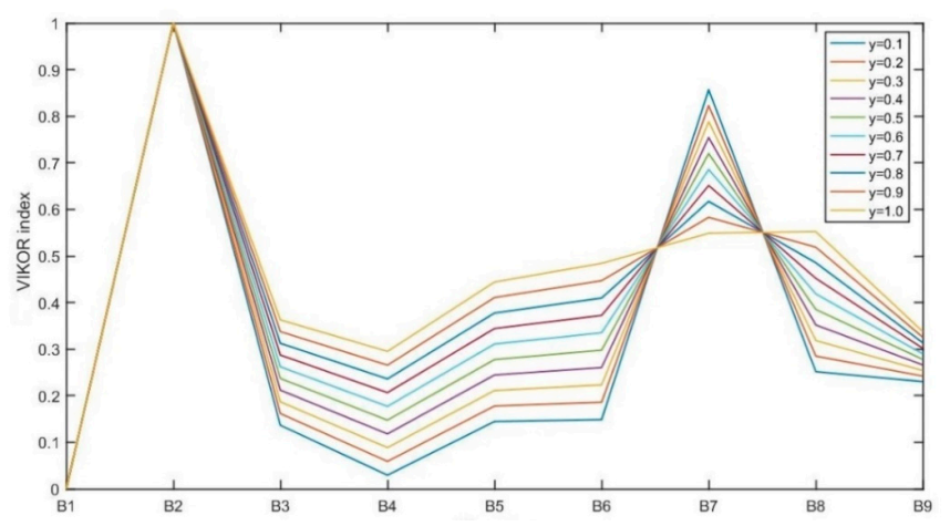
Step 7.Calculation of VIKOR index.

Hereby, the VIKOR index is defined, taking into account rough neutrosophic characteristics of utility and regret measure, and the decision-making mechanism coefficient $\gamma$ is considered from 0 to 1.

$${\mathsf{\Phi }}_i=\gamma \left|\left(\frac{RN{S}_i-RN{S}_i{}^{-}}{RN{S}_i{}^{+}-RN{S}_i{}^{-}}\right)\right|+\left(1-\gamma \right)\left|\left(\frac{RN{Z}_i-RN{Z}_i{}^{-}}{RN{Z}_i{}^{+}-RN{Z}_i{}^{-}}\right)\right|$$

(41)

where $RN{S}_i^{-}=\underset{i}{\min }RN{S}_i$, $RN{S}_i^{+}=\underset{i}{\max }RN{S}_i$, $RN{Z}_i^{-}=\underset{i}{\min }RN{Z}_i$, $RN{Z}_i^{+}=\underset{i}{\max }RN{Z}_i$, and $\gamma$ is the decision-making mechanism coefficient [64]. For the maximum group utility, $\gamma >0.5,$ and for the minimum group utility, $\gamma <0.5$. The median is taken as $\gamma =0.5$ [50].

The compromise alternative is $A_1$, which has the minimum $\mathsf{\Phi }$ value when two conditions are satisfied [65]:

Condition 1. 

$\mathsf{\Phi }\left(A_2\right)-\mathsf{\Phi }\left(A_1\right)\ge \Psi$, where$A_2$is the second ranked alternative by$\mathsf{\Phi }$in the ranking list, and$\Psi =\frac{1}{n-1}$.

Condition 2. 

If$A_1$is also ranked first by$RNS$and$RNZ$, then it is the most satisfying in the decision-making process.

In the case when one of the conditions is not satisfied, the compromise alternative is obtained by following conditions:

Condition 3. 

$A_1$and$A_2$are considered compromised if Condition 2 is not satisfied, or

Condition 4. 

$A_1, A_2,\dots ,A_n$are considered compromised if Condition 1 is not satisfied, and$A_n$is defined by$\mathsf{\Phi }\left(A_n\right)-\mathsf{\Phi }\left(A_1\right)<\Psi$.

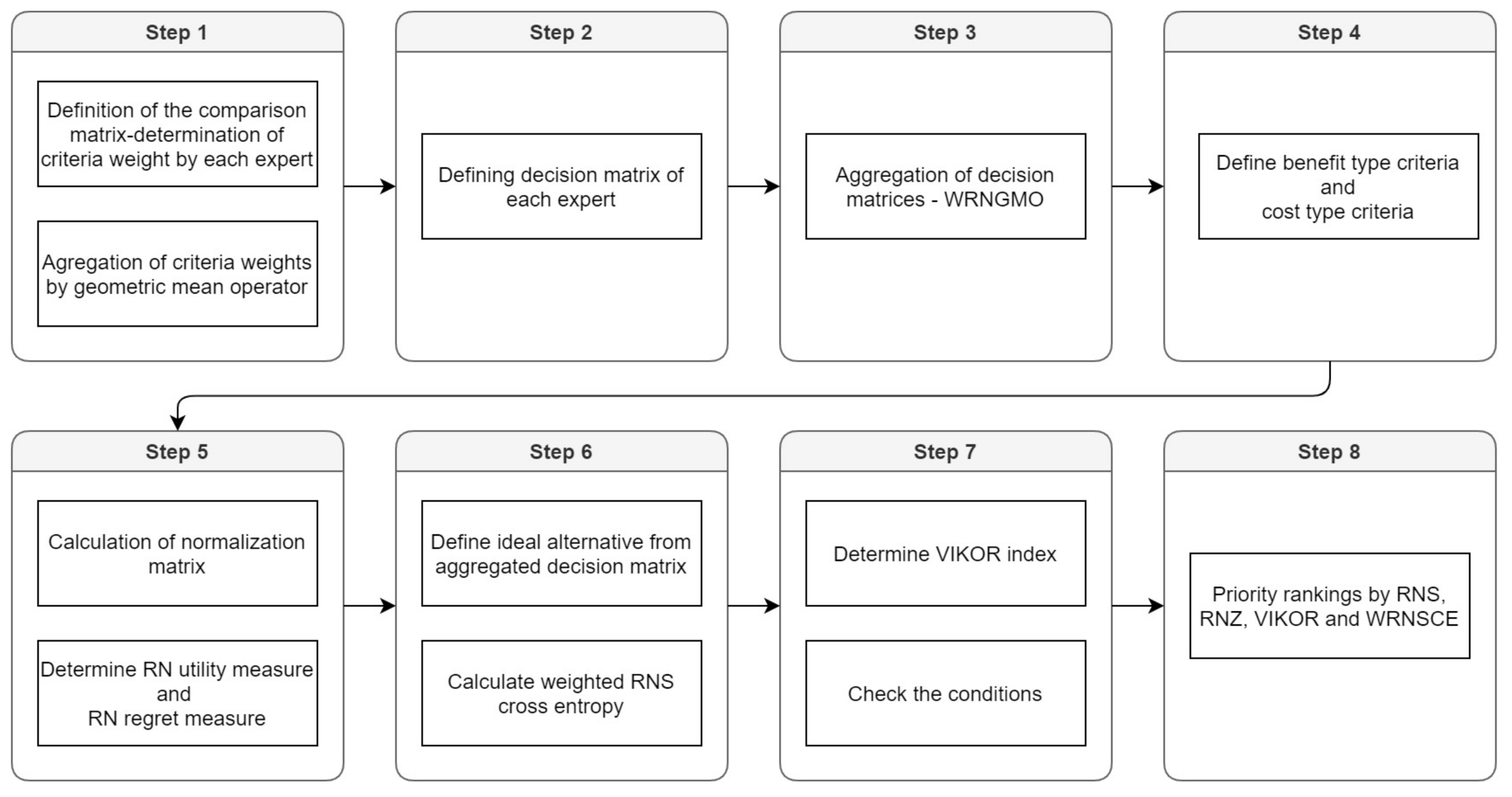
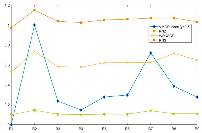
Step 8.Priority ranking.

Priority ranking is defined by $RN{S}_i$, $RN{Z}_i,$ ${\mathsf{\Phi }}_i$ and $WRNSC{E}_i$. Smaller values indicate the higher priority of the alternative. Furthermore, in Figure 1, the proposed methodology is illustratively presented in detail, throughout the framework.

3. Illustrative Example

The proposed methodology is applied on an illustrative example of a multicriteria decision-making problem to distinguish the attainability and capability of strategic planning to the remediation of historic pedestrian bridges. Hereby, nine bridges located in Split-Dalmatia County under the management of the Ministry of Culture of Croatia are evaluated. A criteria list is generated from the study [66], and two more criteria are added, detour (C12) and landscape (C13), which affected the final ranking of bridges. Three experts are introduced to the problem and asked to define criteria weights and alternatives assessments. The following bridges are considered for the remediation: (B1) Kaštilac, Kaštel Gomilica; (B2) Ričevica, Kaštel Štafilić; (B3) the bridge next to the Castel Vitturi, Kaštel Luksic; (B4) the bridge next to the Ćosić mill, Grab; (B5) the bridge next to the Samarđić mill, Grab; (B6) small bridge over the River Grab, Grab; (B7) Goručica, Sinj; (B8) Vrboska, Hvar; (B9) Franjo Josip, Brač.

Step 1.Definition of comparison matrix and aggregation of criteria weights.

A criteria list along with definitions are presented in

Table 1. List of criteria with definition.

Label	Criteria	Definition
C1	Bridge condition	Cost
C2	The complexity of bridge rehabilitation	Benefit
C3	Bridge load	Benefit
C4	Last rehabilitation	Benefit
C5	Rehabilitation cost	Cost
C6	Cost of waste material disposal	Cost
C7	Required time for rehabilitation	Cost
C8	Required time for document preparation	Cost
C9	Preservation of cultural heritage	Benefit
C10	Tourist attraction	Benefit
C11	Historical importance	Benefit
C12	Detour	Cost
C13	Landscape	Benefit

, while in

Table 2. Linguistic values and rough neutrosophic set for criteria comparison.

Linguistic Values	Saaty’s Scale [61]	Rough Neutrosophic Set
Equally important	1	(0.5, 0.5, 0.5; 0.5, 0.5, 0.5)
Slightly important	3	(0.1, 0.85, 0.8; 0.3, 0.75, 0.7)
Strongly important	5	(0.3, 0.75, 0.7; 0.6, 0.35, 0.4)
Very strongly important	7	(0.6, 0.35, 0.4; 0.8, 0.15, 0.2)
Absolutely important	9	(0.9, 0.1, 0.1; 1, 0, 0)
In-between values	2	(0.05, 0.3, 0.25; 0.2, 0.75, 0.7)
	4	(0.2, 0.7, 0.65; 0.4, 0.65, 0.6)
	6	(0.55, 0.6, 0.5; 0.7, 0.25, 0.3)
	8	(0.7, 0.25, 0.3; 0.8, 0.15, 0.2)

the linguistic values and corresponding rough neutrosophic sets for the criteria comparison are given. Sets and linguistic values are defined according to Saaty’s scale [61].

Each expert compared criteria using rough neutrosophic Saaty’s scale from Table 2. Then the criteria weights are calculated by (27) and (28), and aggregated using (29). In

Table 3. Criteria weights by each expert and aggregated weights.

	Expert1	Expert2	Expert3	Aggregated
C1	0.077	0.091	0.110	0.092
C2	0.075	0.079	0.079	0.078
C3	0.074	0.086	0.086	0.082
C4	0.092	0.060	0.079	0.076
C5	0.069	0.071	0.085	0.075
C6	0.083	0.090	0.099	0.090
C7	0.087	0.075	0.080	0.081
C8	0.073	0.065	0.068	0.069
C9	0.075	0.087	0.093	0.084
C10	0.064	0.070	0.070	0.068
C11	0.086	0.086	0.089	0.087
C12	0.083	0.095	0.098	0.092
C13	0.060	0.100	0.101	0.085

, weights provided by each expert and aggregated weights are presented.

Step 2.Determination of RN decision matrix.

The assessments of alternatives $B_i \left(i=1,2,\dots ,9\right)$by each criterion $C_i \left(i=1,2,\dots ,13\right)$ are given by the experts $E_l \left(l=1, 2, 3\right)$ forming decision matrices.

Table 4. Linguistic values and rough neutrosophic sets for alternatives’ assessment.

Linguistic Value	Rough Neutrosophic Set
Extreme high (EH)	(0.95, 0.05, 0.05; 1, 0, 0)
Very very high (VVH)	(0.85, 0.05, 0.05; 0.9, 0.1, 0.1)
Very high (VH)	(0.75, 0.1, 0.15; 0.8, 0.15, 0.2)
High (H)	(0.65, 0.2, 0.25; 0.7, 0.25, 0.3)
Medium high (MH)	(0.55, 0.3, 0.35; 0.6, 0.35, 0.4)
Medium poor (MP)	(0.45, 0.5, 0.5; 0.5, 0.45, 0.5)
Poor (P)	(0.35, 0.6, 0.55; 0.4, 0.65, 0.6)
Very poor (VP)	(0.25, 0.65, 0.6; 0.3, 0.7, 0.65)
Very very poor (VVP)	(0.15, 0.7, 0.65; 0.2, 0.75, 0.7)
Extreme poor (EP)	(0.05, 0.8, 0.75; 0.1, 0.85, 0.8)

provides linguistic values and rough neutrosophic sets for the assessment of alternatives. Experts’ judgements are presented in

Table A1. Assessment of alternatives by E1.

	C1	C2	C3	C4	C5	C6	C7	C8	C9	C10	C11	C12	C13
B1	MH	VP	VH	VVH	VH	VH	VH	VH	EH	VVH	VVH	VP	VVH
B2	MH	VP	MH	MH	MH	MH	MH	MH	EP	VH	P	VVH	VVH
B3	MH	VP	MH	MH	MH	VH	VH	VH	EH	VVH	VVH	EP	VVH
B4	MH	VP	MH	VVH	H	H	H	H	EH	VVH	VVH	VP	VVH
B5	H	VP	MH	MH	MH	MP	MP	MP	EH	VVH	VVH	VVH	VVH
B6	H	VP	VH	MH	MH	MH	MH	MH	EH	VVH	VVH	VVP	VVH
B7	H	VP	VVH	H	H	H	H	H	EH	VH	VVH	VP	P
B8	H	VP	P	VH	MH	MH	MH	MH	EH	VVH	VVH	VP	VVH
B9	VH	VVP	P	VH	H	H	H	H	EH	VVH	VVH	VVP	VVH

,

Table A2. Assessment of alternatives by E2.

	C1	C2	C3	C4	C5	C6	C7	C8	C9	C10	C11	C12	C13
B1	MH	VP	VH	VVH	VH	VH	VH	VH	EH	VVH	VVH	VP	VVH
B2	MH	VP	MH	MH	MH	MH	MH	MH	EP	H	P	VVH	VVH
B3	MH	VP	MH	MH	MH	VH	VH	VH	EH	VVH	VVH	EP	VVH
B4	MH	VP	MH	VVH	MH	H	H	H	EH	VVH	VVH	VP	VVH
B5	H	VVP	MH	MH	MH	P	MP	MP	EH	VVH	VVH	VVH	VVH
B6	MH	VP	VH	MH	MH	MH	MH	MH	EH	VVH	VVH	VVP	VVH
B7	MH	VP	VVH	H	H	MH	H	H	EH	VVH	VVH	VP	MP
B8	H	P	P	VH	MH	MH	MH	MH	EH	VVH	VVH	VP	VVH
B9	VH	P	P	VH	H	H	H	H	EH	VVH	VVH	VVP	VVH

and

Table A3. Assessment of alternatives by E3.

	C1	C2	C3	C4	C5	C6	C7	C8	C9	C10	C11	C12	C13
B1	MH	VP	VH	VVH	VH	VH	VH	VH	EH	VVH	VVH	VVP	VVH
B2	H	P	MH	MH	MH	MH	MH	MH	EP	VH	P	VVH	VVH
B3	MH	VP	MH	MH	MH	VH	VH	VH	EH	VVH	VVH	EP	VVH
B4	H	P	MH	VVH	H	H	H	H	EH	VVH	VVH	VVP	VVH
B5	H	P	MH	MH	MH	MP	MP	MP	EH	VVH	VVH	VVH	VVH
B6	H	VP	VH	MH	MH	MH	MH	MH	EH	VVH	VVH	VP	VVH
B7	H	VP	VVH	H	H	H	H	H	EH	VVH	VVH	VP	P
B8	H	VP	P	VH	MH	MH	MH	MH	EH	VVH	VVH	VP	VVH
B9	VH	VVP	P	VH	H	H	H	H	EH	VVH	VVH	VP	VVH

with linguistic values, and given in the Appendix A.

Step 3.Aggregation of RN decision matrices.

Using Expression (31), the RN weighted aggregated decision matrix by each criterion is calculated as follows:

$C1$	$C2$	$C3$
$\begin{array}{c}B1\\ B2\\ B3\\ B4\\ B5\\ B6\\ B7\\ B8\\ B9\end{array}\left(\begin{array}{cccccc}1.04& 0.72& 0.75& 1.04& 0.75& 0.78\\ 1.04& 0.69& 0.73& 1.05& 0.73& 0.76\\ 1.04& 0.72& 0.75& 1.04& 0.75& 0.78\\ 1.04& 0.69& 0.73& 1.05& 0.73& 0.76\\ 1.05& 0.64& 0.68& 1.05& 0.68& 0.72\\ 1.05& 0.67& 0.70& 1.05& 0.70& 0.74\\ 1.05& 0.67& 0.70& 1.05& 0.70& 0.74\\ 1.05& 0.64& 0.68& 1.05& 0.68& 0.72\\ 1.06& 0.53& 0.59& 1.06& 0.59& 0.64\end{array}\right)$	$\begin{array}{c}B1\\ B2\\ B3\\ B4\\ B5\\ B6\\ B7\\ B8\\ B9\end{array}\left(\begin{array}{cccccc}0.98& 0.90& 0.89& 0.99& 0.92& 0.90\\ 0.99& 0.90& 0.88& 1.00& 0.92& 0.90\\ 0.98& 0.90& 0.89& 0.99& 0.92& 0.90\\ 0.99& 0.90& 0.88& 1.00& 0.92& 0.90\\ 1.00& 0.89& 0.87& 1.01& 0.90& 0.89\\ 0.98& 0.90& 0.89& 0.99& 0.92& 0.90\\ 0.98& 0.90& 0.89& 0.99& 0.92& 0.90\\ 0.98& 0.90& 0.89& 0.99& 0.92& 0.90\\ 0.94& 0.92& 0.90& 0.96& 0.94& 0.92\end{array}\right)$	$\begin{array}{c}B1\\ B2\\ B3\\ B4\\ B5\\ B6\\ B7\\ B8\\ B9\end{array}\left(\begin{array}{cccccc}1.05& 0.57& 0.63& 1.05& 0.63& 0.67\\ 1.03& 0.74& 0.77& 1.04& 0.77& 0.80\\ 1.03& 0.74& 0.77& 1.04& 0.77& 0.80\\ 1.03& 0.74& 0.77& 1.04& 0.77& 0.80\\ 1.03& 0.74& 0.77& 1.04& 0.77& 0.80\\ 1.05& 0.57& 0.63& 1.05& 0.63& 0.67\\ 1.06& 0.48& 0.48& 1.06& 0.57& 0.57\\ 1.00& 0.88& 0.86& 1.01& 0.90& 0.88\\ 1.00& 0.88& 0.86& 1.01& 0.90& 0.88\end{array}\right)$
$C4$	$C5$	$C6$
$\begin{array}{c}B1\\ B2\\ B3\\ B4\\ B5\\ B6\\ B7\\ B8\\ B9\end{array}\left(\begin{array}{cccccc}1.05& 0.51& 0.51& 1.05& 0.59& 0.59\\ 1.03& 0.76& 0.79& 1.04& 0.79& 0.81\\ 1.03& 0.76& 0.79& 1.04& 0.79& 0.81\\ 1.05& 0.51& 0.51& 1.05& 0.59& 0.59\\ 1.03& 0.76& 0.79& 1.04& 0.79& 0.81\\ 1.03& 0.76& 0.79& 1.04& 0.79& 0.81\\ 1.04& 0.69& 0.73& 1.04& 0.73& 0.76\\ 1.05& 0.59& 0.65& 1.05& 0.65& 0.69\\ 1.05& 0.59& 0.65& 1.05& 0.65& 0.69\end{array}\right)$	$\begin{array}{c}B1\\ B2\\ B3\\ B4\\ B5\\ B6\\ B7\\ B8\\ B9\end{array}\left(\begin{array}{cccccc}1.05& 0.60& 0.65& 1.05& 0.65& 0.70\\ 1.03& 0.76& 0.79& 1.04& 0.79& 0.81\\ 1.03& 0.76& 0.79& 1.04& 0.79& 0.81\\ 1.04& 0.70& 0.73& 1.04& 0.73& 0.76\\ 1.03& 0.76& 0.79& 1.04& 0.79& 0.81\\ 1.03& 0.76& 0.79& 1.04& 0.79& 0.81\\ 1.04& 0.70& 0.73& 1.04& 0.73& 0.76\\ 1.03& 0.76& 0.79& 1.04& 0.79& 0.81\\ 1.04& 0.70& 0.73& 1.04& 0.73& 0.76\end{array}\right)$	$$\begin{gathered} \begin{array}{c}B1\\ B2\\ B3\\ B4\\ B5\\ B6\\ B7\\ B8\\ B9\end{array}\left(\begin{array}{cccccc}1.06& 0.54& 0.60& 1.06& 0.60& 0.65\\ 1.04& 0.72& 0.75& 1.04& 0.75& 0.78\\ 1.06& 0.54& 0.60& 1.06& 0.60& 0.65\\ 1.05& 0.65& 0.69& 1.05& 0.69& 0.72\\ 1.02& 0.83& 0.83& 1.03& 0.81& 0.83\\ 1.04& 0.72& 0.75& 1.04& 0.75& 0.78\\ 1.05& 0.65& 0.69& 1.05& 0.69& 0.72\\ 1.04& 0.72& 0.75& 1.04& 0.75& 0.78\\ 1.05& 0.65& 0.69& 1.05& 0.69& 0.72\end{array}\right) \\ C7 \end{gathered}$$
$C7$	$C8$	$C9$
$\begin{array}{c}B1\\ B2\\ B3\\ B4\\ B5\\ B6\\ B7\\ B8\\ B9\end{array}\left(\begin{array}{cccccc}1.05& 0.57& 0.63& 1.05& 0.63& 0.68\\ 1.03& 0.75& 0.78& 1.04& 0.78& 0.80\\ 1.05& 0.57& 0.63& 1.05& 0.63& 0.68\\ 1.04& 0.68& 0.72& 1.05& 0.72& 0.75\\ 1.02& 0.85& 0.85& 1.03& 0.82& 0.85\\ 1.03& 0.75& 0.78& 1.04& 0.78& 0.80\\ 1.04& 0.68& 0.72& 1.05& 0.72& 0.75\\ 1.03& 0.75& 0.78& 1.04& 0.78& 0.80\\ 1.04& 0.68& 0.72& 1.05& 0.72& 0.75\end{array}\right)$	$\begin{array}{c}B1\\ B2\\ B3\\ B4\\ B5\\ B6\\ B7\\ B8\\ B9\end{array}\left(\begin{array}{cccccc}1.04& 0.62& 0.68& 1.04& 0.68& 0.72\\ 1.03& 0.78& 0.81& 1.03& 0.81& 0.83\\ 1.04& 0.62& 0.68& 1.04& 0.68& 0.72\\ 1.04& 0.72& 0.75& 1.04& 0.75& 0.78\\ 1.02& 0.87& 0.87& 1.02& 0.85& 0.87\\ 1.03& 0.78& 0.81& 1.03& 0.81& 0.83\\ 1.04& 0.72& 0.75& 1.04& 0.75& 0.78\\ 1.03& 0.78& 0.81& 1.03& 0.81& 0.83\\ 1.04& 0.72& 0.75& 1.04& 0.75& 0.78\end{array}\right)$	$\begin{array}{c}B1\\ B2\\ B3\\ B4\\ B5\\ B6\\ B7\\ B8\\ B9\end{array}\left(\begin{array}{cccccc}1.06& 0.84& 0.84& 1.06& 0.00& 0.00\\ 0.85& 0.95& 0.93& 0.90& 0.96& 0.95\\ 1.06& 0.84& 0.84& 1.06& 0.00& 0.00\\ 1.06& 0.84& 0.84& 1.06& 0.00& 0.00\\ 1.06& 0.84& 0.84& 1.06& 0.00& 0.00\\ 1.06& 0.84& 0.84& 1.06& 0.00& 0.00\\ 1.06& 0.84& 0.84& 1.06& 0.00& 0.00\\ 1.06& 0.84& 0.84& 1.06& 0.00& 0.00\\ 1.06& 0.84& 0.84& 1.06& 0.00& 0.00\end{array}\right)$
$C10$	$C11$	$C12$
$\begin{array}{c}B1\\ B2\\ B3\\ B4\\ B5\\ B6\\ B7\\ B8\\ B9\end{array}\left(\begin{array}{cccccc}1.05& 0.54& 0.54& 1.05& 0.62& 0.62\\ 1.05& 0.54& 0.54& 1.05& 0.62& 0.62\\ 1.05& 0.54& 0.54& 1.05& 0.62& 0.62\\ 1.05& 0.54& 0.54& 1.05& 0.62& 0.62\\ 1.05& 0.54& 0.54& 1.05& 0.62& 0.62\\ 1.05& 0.54& 0.54& 1.05& 0.62& 0.62\\ 1.05& 0.54& 0.54& 1.05& 0.62& 0.62\\ 1.05& 0.54& 0.54& 1.05& 0.62& 0.62\\ 1.05& 0.54& 0.54& 1.05& 0.62& 0.62\end{array}\right)$	$\begin{array}{c}B1\\ B2\\ B3\\ B4\\ B5\\ B6\\ B7\\ B8\\ B9\end{array}\left(\begin{array}{cccccc}1.06& 0.46& 0.46& 1.06& 0.55& 0.55\\ 1.00& 0.88& 0.86& 1.01& 0.89& 0.88\\ 1.06& 0.46& 0.46& 1.06& 0.55& 0.55\\ 1.06& 0.46& 0.46& 1.06& 0.55& 0.55\\ 1.06& 0.46& 0.46& 1.06& 0.55& 0.55\\ 1.06& 0.46& 0.46& 1.06& 0.55& 0.55\\ 1.06& 0.46& 0.46& 1.06& 0.55& 0.55\\ 1.06& 0.46& 0.46& 1.06& 0.55& 0.55\\ 1.06& 0.46& 0.46& 1.06& 0.55& 0.55\end{array}\right)$	$\begin{array}{c}B1\\ B2\\ B3\\ B4\\ B5\\ B6\\ B7\\ B8\\ B9\end{array}\left(\begin{array}{cccccc}0.97& 0.89& 0.87& 0.99& 0.91& 0.89\\ 1.06& 0.44& 0.44& 1.06& 0.53& 0.53\\ 0.84& 0.94& 0.92& 0.90& 0.96& 0.94\\ 0.97& 0.89& 0.87& 0.99& 0.91& 0.89\\ 1.06& 0.44& 0.44& 1.06& 0.53& 0.53\\ 0.93& 0.91& 0.89& 0.95& 0.92& 0.91\\ 0.97& 0.89& 0.87& 0.99& 0.91& 0.89\\ 0.97& 0.89& 0.87& 0.99& 0.91& 0.89\\ 0.93& 0.91& 0.89& 0.95& 0.92& 0.91\end{array}\right)$
	$C13$
	$\begin{array}{c}B1\\ B2\\ B3\\ B4\\ B5\\ B6\\ B7\\ B8\\ B9\end{array}\left(\begin{array}{cccccc}1.06& 0.47& 0.47& 1.06& 0.56& 0.56\\ 1.06& 0.47& 0.47& 1.06& 0.56& 0.56\\ 1.06& 0.47& 0.47& 1.06& 0.56& 0.56\\ 1.06& 0.47& 0.47& 1.06& 0.56& 0.56\\ 1.06& 0.47& 0.47& 1.06& 0.56& 0.56\\ 1.06& 0.47& 0.47& 1.06& 0.56& 0.56\\ 1.00& 0.88& 0.86& 1.01& 0.90& 0.88\\ 1.06& 0.47& 0.47& 1.06& 0.56& 0.56\\ 1.06& 0.47& 0.47& 1.06& 0.56& 0.56\end{array}\right)$

Step 4.Definition of benefit type criteria and cost type criteria.

Benefit and cost type criteria are calculated using (34) and (35).

Benefit type criteria:

$$C2=\left(1.001, 0.888, 0.870;0.960, 0.905, 0.920\right),$$

$$C3=\left(1.055, 0.480, 0.480;1.010, 0.569, 0.882\right),$$

$$C4=\left(1.051, 0.506, 0.506;1.036, 0.592, 0.812\right),$$

$$C9=\left(1.060, 0.839, 0.839;0.903, 0.000, 0.945\right),$$

$$C10=\left(1.046, 0.542, 0.542;1.047, 0.625, 0.625\right),$$

$$C11=\left(1.059, 0.458, 0.458;1.011, 0.549, 0.875\right),$$

$$C13=\left(1.057, 0.467, 0.467;1.011, 0.557, 0.878\right)$$

Cost type criteria:

$$C1=\left(1.037, 0.718, 0.749;1.060, 0.749, 0.642\right),$$

$$C5=\left(1.030, 0.763, 0.790;1.049, 0.790, 0.697\right),$$

$$C6=\left(1.021, 0.829, 0.829;1.059, 0.805, 0.646\right),$$

$$C7=\left(1.019, 0.846, 0.846;1.052, 0.825, 0.678\right),$$

$$C8=\left(1.016, 0.867, 0.867;1.45, 0.848, 0.718\right),$$

$$C12=\left(0.840, 0.940, 0.924;1.064, 0.956, 0.531\right)$$

Step 5.Defintion of RN utility measure and RN regret measure.

Firstly, normalization is calculated using (37), then the RN utility measure (RNS) and the RN regret measure (RNZ) are determined using (38) and (39), respectively. RNS and RNZ are given as follows:

RNS:

$$B1=0.974, B2=1.149, B3=1.037, B4=1.026, B5=1.052, B6=1.059, B7=1.070,$$

$$B8=1.071,B9=1.033$$

RNZ:

$$B1=0.101, B2=0.145, B3=0.106, B4=0.101, B5=0.106, B6=0.106, B7=0.140,$$

$$B8=0.110,B9=0.110$$

Step 6.Calculating the weighted RNS cross entropy.

Using Expressions (22) and (40), weighted RNS cross entropy is calculated between the ideal alternative and weighted aggregated decision matrix. Values of weighted RNS cross entropy are presented as follows:

WRNSCE:

$$B1=0.528, B2=0.736, B3=0.584, B4=0.578, B5=0.622, B6=0.624, B7=0.625,$$

$$B8=0.715,B9=0.651$$

Step 7.Calculation of VIKOR index.

After the calculation of RNS and RNZ, values of the VIKOR index are defined for the decision-making mechanism coefficient $\gamma ,$ ranging from 0 to 1. These values are presented in Figure 2. According to the VIKOR index, B1 has the lowest value for each decision-making mechanism coefficient, while B2 has the highest.

Step 8.Priority ranking.

From the previous step and Figure 2, it is obvious that the B1 alternative is the most suitable for the remediation, with the value of $\mathsf{\Phi }=0$ for each $\gamma$ value, and B2 is least suitable, with $\mathsf{\Phi }=1$. Furthermore, the relations between the values of RNS, RNZ, WRNSCE and VIKOR index, for $\gamma =0.5$, are presented in Figure 2. The given relations are used to define and compare rankings. The bridges are ranked by RNS, RNZ, WRNSCE and VIKOR index values as follows:

$$\mathrm{RNS}: B1>B4>B9>B3>B5>B6>B7>B8>B2$$

$$\mathrm{RNZ}: B1>B4>B3>B5>B6>B8>B9>B7>B2$$

$$\mathrm{WRNSCE}: B1>B4>B3>B5>B6>B7>B9>B8>B2$$

$$\mathrm{VIKOR} (\gamma =0.5):B1>B4>B3>B5>B9>B6>B8>B7>B2$$

According to each presented ranking, B1 is ranked first and B2 last. In this way, Condition 1 and Condition 2 are satisfied, where $\mathsf{\Phi }\left(0.148\right)-\mathsf{\Phi }\left(0\right)\ge 0.125$, and B1 is also the most optimal solution according to the RNS and RNZ values. In Figure 3, the given relations between RNS, RNZ, WRNSCE and the VIKOR index present the obtained rankings where the similarity in rankings between values is high, especially between WRNSCE and $\mathsf{\Phi }$. Hence, combining the VIKOR method and cross entropy under rough neutrosophic set theory can gain more precise and certain outcomes. By adding two new criteria, the final rankings show deviation between these approaches, but B1 is still the most suitable for the remediation, and B2 is at the bottom of the ranking list. In addition, different experts were involved in the process of criteria definition and alternative assessments. The comparison of the values of WRNSCE, the VIKOR index and the AHP-evidential reasoning-TOPSIS approach are given in Figure 4.

Furthermore, similarity and comparison between rankings is also numerically presented by $r_w$ (weighted Spearman’s rank correlation coefficient) and $WS$ (rank similarity coefficient), defined in [42]. Both coefficients are calculated to compare the rankings of WRNSCE and the VIKOR index with reference ranking obtained by [65]. The weighted Spearman’s rank correlation coefficient examines the appearance of differences, not in which place they appear, while the rank similarity coefficient is based on the position significance of reference ranking during determination [46]. In

Table 5. Comparison of the rankings obtained by WRNSCE and the VIKOR index with reference ranking using $r_w$ and $WS$.

Coefficient	WRNSCE	VIKOR Index
$r_s$	0.33	0.44
$WS$	0.66	0.73

, $r_w$ and $WS$ are calculated as a numerical presentation of similarity between rankings achieved by WRNSCE and the VIKOR index with the reference ranking.

The obtained results show the correlation between the observed rankings, and from Table 5, it is obvious that the ranking achieved by the VIKOR index is similar to the reference ranking by $r_s$ and $WS$ values. It should be emphasized that that the reference ranking is obtained with a smaller number of criteria ($N=11)$, used to evaluate alternatives. In addition, in reference ranking, different evaluation measures are included in alternatives assessment and criteria weights determination, while not paying much attention to the uncertainty, inconsistency and incompleteness of information. In addition, different experts are included in the proposed methodology. These mentioned factors lead to a slightly lower correlation between the reference rankings and the rankings obtained by developed model.

4. Conclusions

In this research, a novel model for multicriteria decision-making is proposed and illustrated based on the example of the strategic planning of historic pedestrian bridge remediation. The model is defined by newly developed cross entropy combined with the VIKOR method under the rough neutrosophic set environment. The newly developed cross entropy under rough neutrosophic set theory does not contain the shortcomings of asymmetrical character and unknown occurrences. Its basic properties are proven and it is established that it can cope with unknown criteria weights. Furthermore, the weighted rough neutrosophic cross entropy has also been developed, and its basic properties are proven.

The VIKOR method under rough neutrosophic set theory is defined. This way, integrating cross entropy, VIKOR, and rough neutrosophic theory, a new model of multicriteria decision-making strategy is developed as a support in the process of decision making. The rankings are calculated using the proposed methodology and defined by values of the VIKOR index, WRNSCE measures, and RNZ and RNS values. These rankings are mutually compared, and according to each of them, the B1 alternative is ranked the most suitable, which proves the efficiency of the model, since Kaštilac bridge is the most deteriorated and most suitable for remediation. The model is compared with the study by Rogulj, Kilić Pamuković, and Jajac [66], where the same alternatives were evaluated, but two extra criteria are added, as was decided by three experts that examined the bridges. What differs between these two methodologies and gives the advantage to the newly proposed method is that the existing study does not include the vagueness and uncertainty of the decision-making problems, and does not use more robust tools and forms of artificial intelligence when dealing with such a real-life complex problem, rather using a classical methodology of multicriteria analysis. The proposed model has proven to be practical, applicable, and efficient when coping with the high demand multicriteria decision-making strategies.

In future research directions, the proposed cross entropy and VIKOR method under rough neutrosophic set theory can be extended to the hypercomplex rough neutrosophic set environment. In addition, a new model based on intuitionistic fuzzy theory will be developed to determine the risk ranking of historic bridges under the significant impact of deterioration and degradation. A new algorithm for a consistency measure of criteria weights and a model for alternative assessment calculation will be proposed.