Abstract
In this paper, we propose presenting a solution based on socio-epidemiological variables of tuberculosis, considering a clustering with spatial/geographical constraints; and, determine a value of alpha that increases spatial contiguity without significantly deteriorating the quality of the solution based on the variables of interest, i.e., those of the feature space. For the application of Ward’s hierarchical clustering method, two dissimilarity matrices were calculated, the first provides the dissimilarities in the feature space calculated from the socio-epidemiological variables and the second provides the dissimilarities in the calculated constraints space from the geographical distances , together with an mixing parameter and the non-uniform weight w assigned to the calculation of the dissimilarity matrix defined by the standardized incidence ratio (SIR) of TB and that contributed significantly to the increase in clarity, both from a spatial and socio-epidemiological point of view. The method is shown to be feasible in epidemiological studies in the joint understanding of factors of different dimensions, aggregated from a spatial perspective. It is analysis tool that allows making a better understanding of the socio-epidemiological reality of the municipality.
1. Introduction
In exploratory data analysis, the statistician often uses clustering and visualization to improve his knowledge of the data [1]. In the viewing, he looks for some clusterings explaining some of the significant characteristics of the data.
The cluster analysis goal consists of distinguishing, in the data set to be analyzed, the groups, called clusters. In this paper, we study the hierarchical clustering (and not partitioning). Hierarchical cluster algorithm groups the data based on the distance between each one and looks for data within a cluster to be the most similar to each other. These groups are disjoint subsets of the data set. They have such a property that data that belong to different clusters differ among themselves much more than the data on the same cluster [2]. The difficulty of choosing the clustering method for grouping a set of n objects into k separate sets and the ideal number of clusters is well frequent among researchers. In Tuberculosis (TB) epidemiology, for instance, this challenge is excellent for being a data-driven approach involving many subjective decisions. However, in some clustering problems, it is relevant to impose constraints on the set of allowed solutions [3]. Contiguity constraints (in space or time) are the most common; they occur when the objects in a cluster required not only to be similar to one other, but also to comprise a contiguous set of objects.
TB still poses a substantial global health threat, with some 10-million new cases per year. In Brazil, the estimate is that the incidence of TB is increasing after many years of decline due to the upward trend in the period of 2016–2018 [4]. TB incidence is disproportionately high among people in poverty [5]. The goal set by the World Health Organization (WHO) is to cure 85% of new bacilliferous TB cases by 2020 [6]; however, as observed in the 2018 data, Brazil (71.4%) falls short of reaching this goal [7]. In the State of Paraíba, the situation is even more critical [8] identified a cure rate of 55% in the studied period (2007–2016).
The State of Paraíba is composed of 223 municipalities; it has the fourteenth contingent population among Brazil’s states with more than 4.018 million inhabitants according to 2019 estimates by the Brazilian Institute of Geography and Statistics [9].
The relationship between TB and social conditions demands an understanding of the dynamics of this aggravation and its occurrence in the territory [10]. This study aims to present a solution based on socio-epidemiological variables of TB with results being easily visualized on a map while using the ClustGeo package. This method uses Ward-like hierarchical clustering with non-Euclidean dissimilarities and non-uniform weights attributed to the standardized incidence ratio (SIR) of TB in the 223 municipalities of Paraíba and the importance of the constraint in the clustering procedure through the parameter , responsible for controlling the weight of the constraint in the quality of the solution on the variables of interest.
Sometimes we wish to provide disease risk estimates in each of the areas that form partitions of the study region [11]. For instance, to identify changes in morbidity and/or mortality in time or to compare the incidence or prevalence. The standardized incidence ratio (SIR) is one simple measure of disease risk.
2. Material and Methods
2.1. Study Design and Data Sources
The data analyzed in this study are notified cases of TB in the 223 municipalities in the State of Paraíba in the period between 2001 and 2018, using a secondary source, through the database, registered in the Notifiable Diseases Information System [12] and made available on the website of the Informatics Department of the Unified Health System (DATASUS). The data are reported cases of TB in the State of Paraíba; the variables are ratios, divided into epidemiological (new cases, cure, male and female deaths) and social variable (active age (20–64) patients with TB). A matrix was also calculated with the geographic distances between the municipalities and the weight w non-uniform attributed to the calculation of the dissimilarity matrix D, as being the standardized incidence ratio (SIR) of TB in the State of Paraíba.
The data were collected between February–May 2020. Statistical analyses were undertaken in R version 3.6.2 [13]. This study was not submitted to the Research Ethics Committee’s evaluation as it is a survey of secondary data and does not directly involve human beings.
2.2. Constrained Hierarchical Clustering
Usually, the researcher has difficulty of clustering a set of n objects into k disjoint clusters. Soon, many methods proposed finding the best partition according to a homogeneity criterion based on differences, or for a multivariate distribution function mix model. The most common type is the contiguity constraints.
Such constraints occur when the objects in a cluster are required not only to be similar to one other, but also to comprise a contiguous set of objects (municipality), i.e., the contiguity between each pair of objects is given by a matrix , where if the ith and the jth objects are contiguous, and 0 if they are not [3]. An adjacency matrix used to find a connection between the borders of each municipality in the State of Paraíba. Accordingly, two clusters are regarded as contiguous if there are two objects, one from each cluster, which is linked in the contiguity matrix. Several authors in different areas of knowledge have implemented of constrained clustering procedures [14,15,16,17,18,19,20,21]. For instance, Miele et al. [22] proposed a model-based spatially constrained method that embeds the geographical information within an EM regularization framework by adding some constraints to the maximum likelihood estimation of parameters. It is a partitioning method with neighbourhood constraints, while the Ward-like method [3] is a hierarchical clustering (and not partitioning) method, including spatial/geographical constraints (not necessarily neighbourhood constraints) [23].
2.3. Ward-Like Hierarchical Clustering
With algorithm similar to Ward, Ward-like is a constrained hierarchical clustering algorithm that optimizes the convex combination of this criterion calculated with two dissimilarity matrices, and beyond a mixing parameter . The first dissimilarity matrix is constructed from the Manhattan distance matrix between the 223 municipalities performed with the p = 5 variables socio-epidemiological, i.e., the matrix gives the differences in the feature space, and the dissimilarity matrix is constructed from the geographical distance between the 223 municipalities, i.e., the matrix gives the differences in constraint space. The minimized criterion at each stage is a convex combination of the homogeneity criterion calculated with and the homogeneity criterion calculated with . The parameter (the weight of this convex combination) gives the relative importance of as compared to . This parameter controls the weight of the constraint on the quality of the solutions, i.e., for a given value of , the mixing parameter clearly controls the part of pseudo-inertia due to and . The mixed pseudo inertia of the cluster is defined as:
where is the weight of ; and are the normalized dissimilarity between observations i and j in and , respectively. For the choice of we will use two types of spatial constraints (geographical distances and neighborhood contiguity). For the last case, the dissimilarity matrix will be constructed from the corresponding adjacency matrix A, i.e., with , equal to 1 if municipalities i and j are neighbourhood 0 otherwise, by convention. When increases, the homogeneity that is calculated with decreases; conversely, the homogeneity calculated increases with . Therefore, the idea is to determine a value of , which increases the spatial the geographical homogeneity without deteriorating the quality of the solution on the variables of interest too much.
These homogeneities are measurable using the appropriate pseudo within-cluster inertias. To determine a suitable value for the mixing parameter , let us assume that the dissimilarity matrix contains geographical distances between n municipalities, whereas the dissimilarity matrix contains distances that are based on a data matrix of socio-epidemiologic variables measured on these n municipalities. Basically, the notion of proportion of the total mixed (pseudo) inertia explained by the partition in K clusters is . When , the denominator is the (pseudo) total inertia, and the numerator is the (pseudo) within-cluster inertia , both based on the dissimilarity matrix. Therefore, the higher the value of the criterion, the more homogeneous is the partition from the socio-epidemiological point of view; , the denominator is the total inertia (pseudo) and the numerator is the (pseudo) inertia within the cluster , both based on the dissimilarity matrix. Ergo, the higher the value of criterion , the more homogeneous is the partition from the geographical point of view. When assumes a value of , the denominator is a total mixed (pseudo) inertia, and it is not easy to interpret in practice and the numerator is the mixed (pseudo) inertia within the cluster.
With R package ClustGeo (version 2.0) developed by Chavent et al. [3], it is possible to implement this hierarchical clustering algorithm with geographical constraints and choose the mixing parameter provided with two types of spatial constraints (geographical distances and neighbourhood contiguity). Let be the weight of the ith observation for . Let be a dissimilarity matrix associated with the n observations, where is the dissimilarity measure between observations i and j. The function hclustgeo of the ClustGeo package is a wrapper of the usual function . It performs the hierarchical clustering of Ward.D, using a dissimilarity matrix D (which is an object of the class , i.e., an object obtained with the function or a dissimilarity matrix transformed into an object of the class with the function) and the weights of observations as arguments. Here, the standardized incidence ratio (SIR) Equation (4) of TB in the 223 municipalities of the State of Paraíba will be applied as non-uniform weights; ergo each municipality will have its weight. The sum of the heights in the dendrogram is equal to the total pseudo-inertia of the data set. The formula for pseudo-inertia of the Ward-like method is:
where is the weight of . The lower the pseudo-inertia , the more homogeneous are the observations that belong to the cluster . The function hclustgeo is a wrapper of the usual hclust function with the following arguments: (a) distance: (Manhattan distance). is the Manhattan distance matrix between the 223 municipalities performed with the variables socio-epidemiological; (b) distance: . The geographic distances between the municipalities; calculating a distance matrix for geographic points using R through packages: sgeostat (version 1.0–27) [24], geosphere (version 1.5–10) [25], and Imap (version 1.32) [26]. These functions calculate distance matrix for geographic for latitude and longitude points of the center of gravity of the municipalities; (c) Members: . The sum of the heights in the dendrogram is equal to the total pseudo-inertia of the data set Equation (2).
The spirit of the Ward-like hierarchical clustering is to aggregate the two clusters A and B from a given partition in clusters, to that the new partition has minimum mixed within-cluster inertia.
2.4. Manhattan Distance
We opted for the Manhattan distance, because the Ward method has already been generalized for use over non-Euclidean distances. According to Strauss and Maltitz [27], Ward’s clustering algorithm can use it in conjunction with Manhattan distances.
where i and j are the municipalities with .
2.5. Standardized Incidence Ratio
One simple measure of disease risk is the standardized incidence ratio (SIR). For each area , the SIR is defined as the ratio of observed counts to the expected counts.
The expected counts represent the total number of TB cases that one would expect if the population of municipality i behaved the way the population of the State of Paraíba behaves. can be calculated while using indirect standardization as , where is the rate (number of cases divided by population) in stratum j in the standard population, and is the population in stratum j of area i.
3. Results and Discussion
Have been notified 24.258 TB cases in the State of Paraíba from 2001 to 2018. Of this total, 80% were new cases, 65% patients got cured, 46.8% had less than ten years of study, 81.3% were between working age (20–64), and 6,1% mortality, being men (4.2%) and women (1.9%). Clustering approaches are a useful tool to detect patterns in data sets and generate hypotheses regarding potential relationships. Therefore, the role of cluster analysis is to uncover a certain kind of natural structure in the data set [2].
Figure 1 shows the dendrogram of the dissimilarity matrix , i.e., the differences in the feature space of socio-epidemiological variables, which is the Manhattan distance matrix between the 223 municipalities performed with variables socio-epidemiological. To choose the suitable number K of clusters, we focus on the Ward dendrogram based on the socio-epidemiological variables, that is using only.
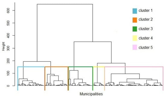
Figure 1.
Dendrogram of the municipalities based on the 5 socio-epidemiologic variables (that is using only).
The visual inspection of the dendrogram in Figure 1 suggests retaining clusters. The 223 municipalities grouped in their respective clusters according to socio-epidemiological similarity, namely, cluster 1 (42 municipalities), cluster 2 (37), cluster 3 (36), cluster 4 (90), and cluster 5, only 18 municipalities. The partition corresponding to the five clusters is shown on the map presented in Figure 2.
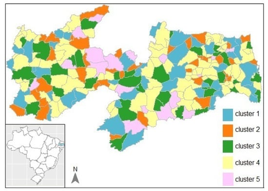
Figure 2.
Map of the partition with 5 clusters only based on the socio-epidemiological variables (that is using only).
Geographically, we perceive clusters well dispersed according to socio-epidemiological variables; that is, the clusters are not strictly contiguous. The interpretation of clusters according to the initial socio-epidemiological variables is interesting. Figure A1 in Appendix A show the variable boxplots for each cluster (top row). Cluster 1, the female mortality rate is the lowest of all clusters, while male mortality has a higher median. Cluster 2 has a high rate of new cases and cure, and a higher female mortality rate than in other clusters. Cluster 3, people of working age (20–64) has a rate that is higher than the average value of the study area, as well as being higher than in other clusters. Similarly, cluster 4 also has a high rate of new cases and a high average age of TB patients of working age and is also greater than the average value of the study area. Cluster 5, high rates of new cases and people of working age, and the lowest cure rate in all other clusters.
We will introduce the matrix of geographical distances into hclustgeo, i.e., a partition taking into account the geographical constraints in order to obtain geographically more compact clusters. For this, it is necessary that a mixing parameter is selected to improve the geographical cohesion of the five groups without adversely affecting the socio-epidemiological cohesion. In Figure 3, we have the mixing parameter defines the importance of and in the clustering process with separate calculations for socio-epidemiologic homogeneity and the geographic cohesion of the partitions obtained for a range of different values of and the five clusters.
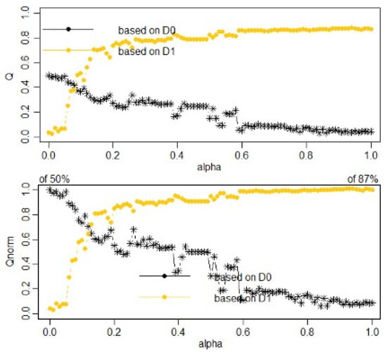
Figure 3.
Choice of for a partition in clusters when is the geographical distances between municipalities. (Top) proportion of explained pseudo-inertias versus (in black solid line) and versus (in gold dashed line). (Bottom) normalized proportion of explained pseudo-inertias versus (in black solid line) and versus (in gold dashed line).
The next plot, Figure 3, shows the choice of for partition, taking into account the geographical constraints.
Figure 3 gives the plot of the proportion of explained pseudo-inertia calculated with (the socio-epidemiological distances), which is equal to 0.50 when and decreases when increases (in solid black line). On the contrary, the proportion of explained pseudo-inertia calculated with (the geographical distances) is equal to 0.87 when and it decreases when decreases (dashed line).
The obtaining of the partition taking into account the geographic constraints with the normalized proportion of explained inertias at the bottom of Figure 3 (i.e., and , shows the value that aims to increase the spatial contiguity, as seen in detail in Table 1.

Table 1.
Normalized proportion of explained pseudo-inertias.
The value of is a trade-off between the loss of socio-economic homogeneity and the gain of geographic cohesion. When , the geographical dissimilarities are not taken into account. When , it is the socio-epidemiologic distances that are not taken into account; the clusters are obtained with the geographical distances only. The plot presented in Figure 3 (bottom) would appear to suggest choosing , which corresponds to a loss of only (1 − 0.61407565 = 38.59%) of socio-epidemiologic with a SIR of each municipality, and 17.75% increase in geographical homogeneity.
The increased geographical cohesion of this partition can be seen in Figure 4.
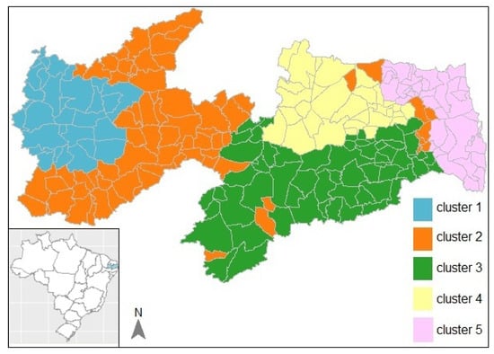
Figure 4.
Map of the partition with clusters based on the socio-epidemiological distances and the geographical distances between the municipalities with .
In Figure 4, a gain significative in spatial homogeneity is perceived. Figure A1 presented in Appendix A shows the boxplots of the variables for each cluster of the partition (middle row). Clusters 1, 3, and 4 seem to differentiate among themselves mainly due to the slight increase in deaths of male patients in cluster 4 and greater variation in the cure proportion of cluster 3. Cluster 5 differed from cluster 2 by the slight increase in deaths, with greater proportions for males, whereas cluster 2 has a higher average number of working-age TB patients and greater variation proportion of cure.
The next plot, Figure 5, shows the choice of for partition, taking into account the neighborhood constraints.
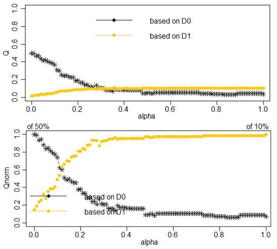
Figure 5.
Choice of for a partition in clusters when is the neighborhood dissimilarity matrix between municipalities. (Top) proportion of explained pseudo-inertias versus (in black solid line) and versus (in gold dashed line). (Bottom) normalized proportion of explained pseudo-inertias versus (in black solid line) and versus (in gold dashed line).
At the bottom of Figure 5, the plot of the normalized proportion of explained inertias (i.e., and ) suggests retaining slightly favoring socio-epidemiological homogeneity versus geographical homogeneity.
It remains only to determine this final partition for clusters and . Figure 6 provides the corresponding map.
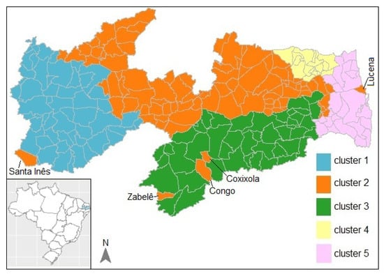
Figure 6.
Map of the partition with clusters based on the socio-epidemiological distances and the “neighborhood” distances of the municipalities with .
Figure 6 shows that the clusters are spatially more compact than those in Figure 5. However, it is known that this approach creates divergences in the adjacency matrix, which gives more importance to the neighborhoods. Thereupon, as the approach is based on soft contiguity restrictions, municipalities that are not neighbours may be in the same clustering, according occurs with the municipalities of Lucena, Coxixola, Congo, Zabelê and Santa Inês in cluster 2. The quality of the partition in Figure 6 is slightly worse than that of the partition in Figure 4, according to the criterion (61.41% versus 82.25%).
4. Conclusions
When considering spatial/geographical constraints, the hierarchical grouping becomes even more complete in detecting patterns in data sets of different dimensions. According to the weights that are given to the geographical differences in this combination, the solution will have more or less spatially contiguous clusters. Through our results, the non-uniform weights w defined by the standardized incidence ratio (SIR) of TB contributed to the increase in clarity both from a spatial and socio-epidemiological point of view.
Therefore, the application of the Ward–Like method becomes indispensable in understanding the socio-epidemiological reality of the State of Paraíba from a spatial perspective, thus facilitating decisions in the development of public policies and more effective health actions in the fight against tuberculosis.
Future work would be to add new socio-epidemiological variables and, instead of the municipalities, use the Health Regions that are responsible for the organization, planning, and execution of health actions and services in the state of Paraíba.
Author Contributions
Resources, D.C.A., R.G.S. and E.L.S.C.; Supervision, R.G.S. and E.L.S.C.; Writing—review & editing, D.C.A. All authors have read and agreed to the published version of the manuscript.
Funding
The research received no external funding.
Conflicts of Interest
The authors declare no conflict of interest.
Abbreviations
The following abbreviations are used in this manuscript:
| DATASUS | Department of the Unified Health System |
| IBGE | Brazilian Institute of Geography and Statistics |
| SIR | standardized incidence ratio |
| TB | tuberculosis |
| WHO | World Health Organization |

References
- Vandewalle, V. Multi-Partitions Subspace Clustering. Mathematics 2020, 8, 597. [Google Scholar] [CrossRef]
- Wierzchoń, S.T.; Kłopotek, M.A. Cluster Analysis. In Modern Algorithms of Cluster Analysis; Janusz, K., Ed.; Springer International Publishing AG: Cham, Switzerland, 2018; pp. 9–66. [Google Scholar]
- Chavent, M.; Kuentz-Simonet, V.; Labenne, A.; Saracco, J. ClustGeo: Hierarchical Clustering with Spatial Constraints, R Package Version 2.0; 2017. Available online: https://CRAN.R-project.org/package=ClustGeo (accessed on 17 May 2020).
- WHO—World Health Organization. Global Tuberculosis Report 2019; World Health Organization: Geneva, Switzerland, 2019. [Google Scholar]
- Reis-Santos, B.; Shete, P.; Bertolde, A.; Sales, C.M.; Sanchez, M.N.; Arakaki-Sanchez, D.; Andrade, K.B.; Gomes, M.G.M.; Boccia, D.; Lienhardt, C.; et al. Tuberculosis in Brazil and Cash Transfer Programs: A Longitudinal Database Study of the Effect of Cash Transfer on Cure Rates. PLoS ONE 2019, 14, e0212617. [Google Scholar] [CrossRef] [PubMed]
- World Health Organization. Global Tuberculosis Report 2017; World Health Organization: Geneva, Switzerland, 2017. [Google Scholar]
- Ministério da Saúde. Brasil Livre da Tuberculose: Evolução dos Cenários Epidemiológicos e Operacionais da Doença; Boletim Epidemiológico; Secretaria de Vigilância em Saúde: Brasília, Brasil, March 2019; Volume 50.
- Aguiar, D.C.; Silva Camelo, E.L.; Carneiro, R.O. Análise estatística de indicadores da tuberculose no Estado da Paraíba. Rev. Aten. Saúde. 2019, 17, 5–12. [Google Scholar]
- IBGE. Instituto brasileiro de geografia e Estatística. In Paraíba–Panorama; 2019. Available online: https://cidades.ibge.gov.br (accessed on 8 May 2020).
- Santos Neto, M.; Sousa, M.R.; da Silva, F.B.G.; Santos, F.S.; Ferreira, A.G.N.; Pascoal, L.M.; Costa, A.C.P.d.; Bezerra, J.M.; Serra, M.A.A.d.O.; Dias, I.C.C.M.; et al. Spatial distribution of tuberculosis cases in a priority Brazilian northeast municipality for control of the disease. Int. J. Dev. Res. 2017, 7, 10611. [Google Scholar]
- Moraga, P. Small Area Disease Risk Estimation and Visualization Using R. R J. 2018, 10, 495–506. [Google Scholar] [CrossRef]
- SINAN. Sistema de Informação de Agravos de Notificação. In Tuberculose–Casos Confirmados; Ministério da Saúde, Brazil: Brasília, Barzil, 2020. Available online: http://www2.datasus.gov.br/ (accessed on 5 April 2020).
- R Core Team. R: A Language and Environment for Statistical Computing; R Foundation for Statistical Computing: Vienna, Austria, 2019; Available online: https://www.R-project.org/ (accessed on 15 May 2020).
- Duque, J.C.; Dev, B.; Betancourt, A.; Franco, J.L. ClusterPy: Library of Spatially Constrained Clustering Algorithms, RiSE-Group (Research in Spatial Economics). 2011. Version 0.9.9; Available online: http://www.rise-group.org/risem/clusterpy/ (accessed on 15 May 2020).
- Bécue-Bertaut, M.; Alvarez-Esteban, R.; Sánchez-Espigares, J.A. Xplortext: Statistical Analysis of Textual Data R Package, R Package Version 1.0. 2017. Version 0.9.9; Available online: https://cran.r-project.org/package=Xplortext (accessed on 7 June 2020).
- Dehman, A.; Ambroise, C.; Neuvial, P. Performance of a blockwise approach in variable selection using linkage disequilibrium information. BMC Bioinform. 2015, 16, 148. [Google Scholar] [CrossRef] [PubMed]
- Legendre, P. const.clust: Space-and Time-Constrained Clustering Package. R Package Version 1.2. 2011. Available online: http://adn.biol.umontreal.ca/numericalecology/Rcode/ (accessed on 20 May 2020).
- Ambroise, C.; Govaert, G. Convergence of an EM-type algorithm for spatial clustering. Pattern Recognit. Lett. 1998, 19, 919–927. [Google Scholar] [CrossRef]
- Ambroise, C.; Dang, M.; Govaert, G. Clustering of Spatial Data by the EM Algorithm. In geoENV I-Geostatistics for Environmental Applicattions; Soares, A.O., Gomez-Hernandez, J.J., Froidevaux, R., Eds.; Kluwer: Dordrecht, The Netherland, 1997; pp. 493–504. [Google Scholar]
- Aguiar, D.C.; Sánchez, R.G.; Silva Camêlo, E.L. Hierarchical clustering with spatial constraints in tuberculosis data. IJDR 2020, 10, 35374–35380. [Google Scholar]
- Aguiar, D.C.; Sánchez, R.G.; Silva Camêlo, E.L. Ward-like hierarchical clustering with dissimilarities and non-uniform weights in cases of tuberculosis in Paraíba, Brazil. IJDR 2020, 10, 35478–35483. [Google Scholar]
- Miele, V.; Picard, F.; Dray, S. Spatially constrained clustering of ecological networks. Methods Ecol. Evol. 2014, 5, 771–779. [Google Scholar] [CrossRef]
- Chavent, M.; Kuentz-Simonet, V.; Labenne, A.; Saracco, J. ClustGeo: An R package for hierarchical clustering with spatial constraints. Comput. Stat. 2018, 33, 1799–1822. [Google Scholar] [CrossRef]
- Majure, J.J.; Gebhardt, A. sgeostat: An Object-Oriented Framework for Geostatistical Modeling in S+, R Package Version 1.0-27; 2016. Available online: https://CRAN.R-project.org/package=sgeostat (accessed on 7 June 2020).
- Hijmans, R.J. Geosphere: Spherical Trigonometry, R Package Version 1.5-10; 2019. Available online: https://CRAN.R-project.org/package=geosphere (accessed on 7 June 2020).
- Wallace, J.R. Imap: Interactive Mapping, R Package Version 1.32; 2012. Available online: https://CRAN.R-project.org/package=Imap (accessed on 7 June 2020).
- Strauss, T.; von Maltitz, M.J. Generalising Ward’s Method for Use with Manhattan Distances. PLoS ONE 2017, 12, e0168288. [Google Scholar] [CrossRef] [PubMed]
© 2020 by the authors. Licensee MDPI, Basel, Switzerland. This article is an open access article distributed under the terms and conditions of the Creative Commons Attribution (CC BY) license (http://creativecommons.org/licenses/by/4.0/).