Stability of Solutions for Parametric Inverse Nonlinear Cost Transportation Problem

Abstract

This paper investigates the solution for an inverse of a parametric nonlinear transportation problem, in which, for a certain values of the parameters, the cost of the unit transportation in the basic problem are adapted as little as possible so that the specific feasible alternative become an optimal solution. In addition, a solution stability set of these parameters was investigated to keep the new optimal solution (feasible one) is unchanged. The idea of this study based on using a tuning parameters $\lambda \in R^m$ in the function of the objective and input parameters $\upsilon \in R^l$ in the set of constraint. The inverse parametric nonlinear cost transportation problem $P(\lambda ,\upsilon )$, where the tuning parameters $\lambda \in R^m$ in the objective function are tuned (adapted) as less as possible so that the specific feasible solution $x^{\circ }$ has been became the optimal ones for a certain values of $\upsilon \in R^l$, then, a solution stability set of the parameters was investigated to keep the new optimal solution $x^{\circ }$ unchanged. The proposed method consists of three phases. Firstly, based on the optimality conditions, the parameter $\lambda \in R^m$ are tuned as less as possible so that the initial feasible solution $x^{\circ }$ has been became new optimal solution. Secondly, using input parameters $\upsilon \in R^l$ resulting problem is reformulated in parametric form $P(\upsilon )$. Finally, based on the stability notions, the availability domain of the input parameters was detected to keep its optimal solution unchanged. Finally, to clarify the effectiveness of the proposed algorithm not only for the inverse transportation problems but also, for the nonlinear programming problems; numerical examples treating the inverse nonlinear programming problem and the inverse transportation problem of minimizing the nonlinear cost functions are presented.

1. Introduction

In the last 20 years, the community of optimization has shown a significant interest in the field of inverse optimization problems. Examples of implementation of inverse optimization in real life have been investigated in various fields such as: traffic, Geophysics, monotonic regression, portfolio and so forth. In any optimization scenario, there are some parameters in the function of the objective and in the functions of the set constraints. When dealing with this problem, generally it is assumed that all these parameters are known but in real situations, there are many cases where the values of the parameters are not precisely known but we may have some fuzzy estimates of the values of these parameters and also have an optimal solution from the past experience or past practice. In these situations, inverse optimization problem can be implemented to adapt the values of the parameters values as less as possible so that the specific solution becomes the optimal one.

Recently, inverse optimization problem is an important new area of investigation involving study and research for the mathematics community [1,2,3,4,5]. In optimization sciences, the coefficients of the cost function are not precisely exactly known; it is truly acceptable to assign a feasible solution $x^{\circ }$ for minimizing objective function nearly optimal, if there exist some nearby cost vector, such that the feasible solution $x^{\circ }$ is an optimal solution for minimizing the objective function. Suppose that the formulation of an optimization problem model consists of a set of optimization parameters (e.g., cost, time,…, etc.), denoted by $\lambda \in R^m$, so we can call these parameters as a tuning parameter, which needs to be tuned so as to $x^{\circ }$ become an optimal solution. Some researcher investigated some applications of inverse optimization problems such as inverse of minimum spanning tree problems and inverse of shortest path problem [5,6,7,8]. Several papers have appeared recently studying some inverse combinatorial problems, where a desired given solution $x^{\circ }$ which is feasible and not an optimal for the model and it is needed to adapt the cost coefficients as little as possible, so that the given solution $x^{\circ }$ becomes a new optimal solution of the model. Some application of the inverse optimization problems is discussed in References [5,6]. Ahuja and Orlin [9] present some studies in the field of inverse optimization problems; also they investigated many applications in network analysis. Zhang and Liu [10] present various inverse linear programming models and they also further investigated it in Reference [11].

Huang and Liu [12] investigated some applications of the inverse of linear programming. Some various applications of the inverse problem have been studied by Amin and Emrouznejad [13]. Inverse linear programming and inverse quadratic programming using perturbation methods was investigated by Zhang et al. [14,15]. Scheafer [16] and Wang [17] discussed the inverse of the integer programming problem. Some basic notions in the convex parametric programming with its qualitative analysis was presented in References [18,19,20], also they discussed the solvability set and stability set.

Transportation problems are considered as special kinds of optimization problems. They present real-world activities that are managed with logistics. it includes transportation with manufacturing products in several supplies to several destinations. The aim is to achieve the minimum total transportation cost that will satisfy the demands at various destinations [21]. Furthermore, a few researchers have been studied variety of inverse transportation problem due to their practical motivation. Implementation of inverse optimization have been applied in various fields [2,3,4,5,6,7,8,9,10,11,12,13,14,15,16,17,18,19,20,21,22,23,24], where it is used to measure operational variance in transit operators, to detect shifts in travel/traffic objectives in system security and risk management, to learn mechanism in autonomous vehicles and so forth. Andrew et al. [24] present a systematic method to derive obscure costs from observations with noisy data of the optimal transportation plans. They implement a formulation of the problem based on graph theory, where nodes represent countries of graphs and assign nonzero weight on the edges between adjacent countries which have a common border. Thai [25] investigate the implementation of inverse optimization to define two types of problems in transportation; he described how inverse optimization and robust optimization can be implemented to find actual time of travel, with noisy information data on travel times. Sanjay et al. [23] investigate the capacitated transportation problem and its inverse; in this problem the transportation cost unit of some products in the basic problem are adapted as less as possible so that the specific feasible solution becomes an optimal solution. Sanjay [26] presents the transportation problem and its inverse, where he investigates the optimizing the ratio of linear objective subject to the set of linear equality constraints and non-negative constraints. Dequan et al. [27] give a brief overview of the inverse optimization problems of the general linear programming (LP). Xu et al. [22] presents a new inverse optimization models and supporting algorithms to learn the parameters of heterogeneous travelers’ route behavior to infer shared network state parameters he proves that the method can obtain unique dual prices for a network shared by these agents in polynomial time.

The main goal of this proposal is to study the stability of solutions for parametric inverse convex nonlinear programming. This work is formal, an advanced extension of our work [28], where the inverse model for nonlinear programming problem NLP are investigated, also different norms L1, L2 and L∞ were implemented in the solution process. The proposed method consists of three phases. Firstly, based on the optimality conditions, tuning parameter $\lambda \in R^m$ is adjusted as less as possible so that the specific initial solution $x^{\circ }$ becomes the new optimal solution. Secondly, with the help of input parameters, $\upsilon \in R^l$ the resulting problem is reformulated in parametric form $P(\upsilon )$. Finally, based on the stability notions, the availability domain of the input parameters was detected to keep its optimal solution unchanged. The proposal is structured as follows. Section 2 introduces problem formulation of the nonlinear transportation. Section 3 discusses the inverse of nonlinear programming problem (NLP). Section 4 investigated the stability notions. Section 5 summarizes the solution procedure. Numerical examples of the inverse optimization problems are described in Section 6. Finally, the results are concluded in the last section.

2. Problem Formulation

Nonlinear transportation problem (NTP) is a special case of nonlinear programming problem (NLP), the formulation of the NTP is more specific, especially in terms of decision variables and the set of constraints. The goal of the nonlinear transportation problem is to optimize (minimize) the vector of nonlinear transportation cost function, in addition to meeting demand, supply and transporting constraints. The standard formulation of the optimization model for the parametric nonlinear transportation problem is given as follows:

$$\begin{array}{l}Minimize\hspace{1em}\hspace{1em}\hspace{1em} C_T={\displaystyle \sum _{r=1}^{m^{\prime }}{\displaystyle \sum _{j=1}^{n^{\prime }}{f}_{rj}({\lambda }_{rj}{x}_{rj}),}}\\ Subject to:\\ \hspace{1em}\hspace{1em}\hspace{1em} {\displaystyle \sum _{j=1}^{n^{\prime }}{x}_{rj}=v_i},r=1,2,\dots ,m^{\prime }\\ \hspace{1em}\hspace{1em}\hspace{1em} {\displaystyle \sum _{r=1}^{m^{\prime }}{x}_{rj}=b_j},j=1,2,\dots ,n^{\prime }\\ \hspace{1em}\hspace{1em}\hspace{1em} x_{rj}\ge 0\hspace{1em}\forall r,j\end{array}$$

(1)

where, objective function variable CT exemplifies the total parametric transportation cost for the transportation problem of a single commodity from sources $m^{\prime }$ to destinations $n^{\prime }$, $f_{rj}({\lambda }_{rj}{x}_{rj})$ denotes the cost function of transporting flow $x_{rj}$ which represent the flow from source i to destination $j, v_r, b_j$ are parametric capacities of each source i and each destination j respectively, ${\lambda }_{ij}\in R^{m^{\prime }+n^{\prime }}$ are set of parameters at the cost function $m^{\prime }$ is the number of sources and $n^{\prime }$ is the number of destination. Problem (1) could be written as a general parametric nonlinear programming problem, which reformulated as follows:

$$\begin{array}{l}P(\lambda ,\upsilon ):\min f(x,\lambda )\\ \hspace{1em}subject to:\\ \hspace{1em}\hspace{1em}\hspace{1em} x\in M=\{x\in R^n|g_i(x,\upsilon )\le 0,i=1,2,\dots k\}\end{array}$$

(2)

where, the objective function $f(x,\lambda )={\displaystyle \sum _{r=1}^{m^{\prime }}{\displaystyle \sum _{j=1}^{n^{\prime }}{f}_{rj}({\lambda }_{rj}{x}_{rj}),}}$ is a convex on $M, \lambda \in R^m$, is a vector of tuning parameters and ${\displaystyle \sum _{j=1}^n{x}_{rj}=a_i},r=1,2,\dots ,m, {\displaystyle \sum _{r=1}^m{x}_{rj}=b_j},j=1,2,\dots ,n ,x_{rj}\ge 0 \forall r,j$ is $g_i(x,\upsilon ),i=1,2,\dots k$ such that $g_i(x,\upsilon ),i=1,2,\dots k$ is a finite-dimensional convex function of class $c^1$ depending on the input parameter $\upsilon \in R^l$. For a predetermined ${\upsilon }^{*}$ (assigned by the decision maker) the problem $P(\lambda ,{\upsilon }^{*})$ is transformed to $P(\lambda )$. Also, it is assumed that $M$ is a non-empty set, such that, the feasibility is guaranteed. Suppose that $f^{*}$ the optimum value for $P(\lambda )$ corresponding to the decision variables $x^{*}$ and tuning parameter ${\lambda }^{*}$. To give the precise formulation of the problem, we present the following definitions.

Definition 1.

Solvability set $S(\lambda )$ of $P(\lambda )$ is defined as:

$$S(\lambda )=\{\lambda \in R^m|\underset{x\in M}{\min } f(x,\lambda ) exists\}.$$

(3)

Let $x^{\circ }$ is the initial solution (feasible) for the problem $P(\lambda )$, knowing that $x^{\circ }$ is not an optimal solution of $P(\lambda )$ problem. In inverse programming, we need to adjust as less as possible the tuning parameter $\lambda$ so that the predetermined initial feasible solution $x^{\circ }$ (which is not an optimal solution for the original model) becomes a new optimal solution of $P({\lambda }^{\circ })$, where ${\lambda }^{\circ }$ is the new value of tuning parameters. First, let us define the expected domain of $\lambda$ which is denoted by $D(\lambda )$, as follows:

Definition 2.

Suppose that ${\lambda }^{}\in S(\lambda )$ with the corresponding optimal solution $x^o$, then we have $D(\lambda )$ which defined by

$$D({\lambda }^o)=\{{\lambda }^o\in S({\lambda }^o)| f(x^o,{\lambda }^o)=\underset{x\in M}{\min } f(x,{\lambda }^o)\}.$$

(4)

Theorem 1.

$D(\lambda )$is nonempty for $P(\lambda )$ the problem.

Proof. 

Since it is assumed that the feasibility is guaranteed for $P(\lambda )$ the problem, that is, $\{\lambda \in R^m|\underset{x\in M}{\min }f(x,\lambda ) exist\}$ then,$D(\lambda )$ is not empty. □

Theorem 2

([29]). Let the solution $(x,\lambda )$ be an initial solution (feasible) of the problem $P(\lambda )$, knowing that $I=\{i:g_i(x)=0\}$, Also, suppose that the two functions $f(.)$ and $g_i(.)$ for $i\in I$ are both differentiable at $(x ,\lambda )$ and that the function $g_i$ is continuous for $i\notin I$ at $(x^{},\lambda )$, then if $(x,{\lambda }^{})$ is a local solution for the problem $P(\lambda )$, then there exist scalars $u_0,u_i$ such that,

$$\begin{array}{l}{u}_o\nabla f(x^o,\lambda )+{\displaystyle \sum _{i\in I}{u}_i\nabla g_i(x^o,\lambda )=0},\\ u_o,u_i\ge 0, for \forall i\in I\\ (u_o,u_l)\ne (0,0)\end{array}$$

(5)

where $u_i$ for $i\in I$ are the components of the vector ${\overline{u}}_l$, furthermore, if $g_i(.)$ for $i\notin I$ are also differentiable at $(x,\lambda )$ for, $i\notin I$, then the forgoing conditions can be formulated in the following form:

$$\begin{array}{l}{u}_o\nabla f(x^o,\lambda )+{\displaystyle \sum _{i\in I}{u}_i\nabla g_i(x^o)=0},\\ u_i{g}_i(x^0)=o for i=1,2,\dots ,k\\ u_o,u_i\ge 0, for i=1,2,\dots ,k.\\ ( u_o,u_l)\ne (0,0)\end{array}$$

(6)

where, $u_i for i=1,2,\dots ,k$ are the components of vector $u$.

Proof. 

Since $(x,{\lambda }^{})$ solve $P(\lambda )$ locally, then there exists no vector $\overline{d}$. Such that $\nabla f{(x,\lambda )}^t\overline{d}<0 and \nabla g_i{(x)}^t<0$ for each $i\in I$. Now, let $A$ is a matrix whose rows are $\nabla f{(x,\lambda )}^t\overline{d} and \nabla g_i{(x)}^t$ $i\in I$. By Gordon’s theorem [22], there exists a non-zero vector $\overline{p}\ge 0$ such that $A^t\overline{p}=0$. Denoting the component of $\overline{p}$, $u_0, and u_i$ for $i\in I$, the first part of the result follows, the equivalent form of the necessary conditions is readily obtained by letting $u_i=0$ for $i\notin I$. □

To determine $D(\lambda )$ of $P(\lambda )$ problem, the following theorems are presented.

Theorem 3

([22]). For a certain $\upsilon$, let $(x,\lambda )$ be an initial feasible solution of $P(\lambda )$, knowing that $I=\{i:g_i(x)=0\}$., Suppose that $f(.) and g_i(.)$ for $i\in I$ are differentiable at $(x,\lambda )$ and that $g_i(.)$ for $i\notin I$ is continuous at $(x,\lambda )$. Furthermore, suppose that $\nabla g_i(x)$ for $i\in I$ are linearly independent. If $(x^{},{\lambda }^{})$ solves $P(\lambda )$ locally, then there exist scalars $u_i$ for $i\in I$ such that

$$\begin{array}{c}\nabla f(x^o,\lambda )+{\displaystyle \sum _{i\in I}{u}_i\nabla g_{i}f(x^o,\lambda )=0},\\ u_i\ge 0, \forall i\in I\end{array}$$

(7)

If $g_i(.)$, $i\notin I$ are also differentiable at $(x,\lambda )$, then the forgoing conditions can be reformulated in the following equivalent form:

$$\begin{array}{ll}\nabla f(x^o,\lambda )+{\displaystyle \sum _{i\in I}{\stackrel{⌢}{u}}_i\nabla g_i(x^o,\lambda )=0},& \\ u_i{g}_i(x^0)=o& for ,i=1,2,\dots ,k\\ u_i\ge 0& for ,i=1,2,\dots ,k.\end{array}$$

(8)

Proof. 

By Theorem 2, there exist scalars $u_o,{\stackrel{⌢}{u}}_i$ for $i\in I$, not all equal to zero, such that

$$\begin{array}{c}{u}_o\nabla f(x^o,\lambda )+{\displaystyle \sum _{i\in I}{\stackrel{⌢}{u}}_i\nabla g_i(x^o,\lambda )=0},\\ u_o,{\stackrel{⌢}{u}}_i\ge 0, for i\in I\end{array}$$

(9)

Knowing that, $u_o>0$, because the system (8) would be contradict with the assumption of linear independence of $\nabla g_i(x,\lambda )$ for $i\in I$ if $u_o=0$. The first part of the theorem then follows by letting $u_i=\frac{{\stackrel{⌢}{u}}_i}{u_o}$ for each $i\in I$. The equivalent form of system (6) follows by letting $u_i=0$ for $i\notin I$. □

Now, let the system as follows:

$$\begin{array}{ll}\frac{\partial f(x,{\lambda }^o)}{\partial x_{\alpha }}+{\displaystyle \sum _{i=1}^k{u}_i\frac{\partial g_r(x)}{\partial x_{\alpha }}}=0& ,\alpha =1,2,\dots n, {\lambda }^o\in R^m\\ u_i{g}_i(x)=o& ,i=1,2,\dots ,k\\ u_i\ge 0& ,i=1,2,\dots ,k.\end{array}$$

(10)

From system (9), we can determine $D(\lambda )$. Since, this system (9) represents independence $n+k$ equations in $k+m$ unknowns and $\lambda \in R^m$, which are linear in $u_i,i=1,2,\dots ,k$ and nonlinear in $\lambda$, then we can obtain $u_i,i=1,2,\dots ,k$ and $\lambda$ explicitly after substituting $x$ by $x^o$.

3. Inverse Nonlinear Programming Problem

The purpose of the proposed inverse optimization approach is to adapt the tuning parameter value from ${\lambda }^{*}$ to ${\lambda }^{\circ }$ so that the specific feasible (given) solution $x^{\circ }$ becomes an optimal solution of $P({\lambda }^{\circ })$ by dealing with the problem

$$\begin{array}{ll}IP({\lambda }^{\circ }):& \min \Vert {\lambda }^{\circ }-{\lambda }^{*}\Vert \\ & subject to: D(\lambda )=\{\lambda \in S: f(x^o,{\lambda }^{\circ })=\underset{x\in M}{\min } f(x,{\lambda }^{\circ })\}\end{array}$$

(11)

Let $\Vert \cdot \Vert$ denote a vector norm, such as L1, L2 or L∞ norm and $N$ is a domain of $\lambda$- parameters that satisfy $\{\lambda \in S(\lambda ): f(x^o,\lambda )=\underset{x\in M}{\min } f(x,\lambda )\}$, it is clear that the domain of the inverse nonlinear programming problem is the same domain of $D(\lambda )$, so that problem (11) can be reformulated as follows:

$$\begin{array}{ll}Q(\lambda ):& \min \Vert {\lambda }^o-{\lambda }^{*}\Vert \\ & subject to: {\lambda }^o\in D({\lambda }^o)\end{array}$$

(12)

Definition 3.

The set of optimality solution of problem (12) which represented by $N_{opt}(\lambda ,x^o)$ is defined as follows:$N_{opt}(\lambda ,x^o)=\{\lambda \in R^m|\underset{\lambda \in D(\lambda )}{\min }\Vert \lambda -{\lambda }^{*}\Vert exists\}.$

Note that: $N_{opt}\subset N$

Theorem 4.

The set of optimality solutions $N_{opt}(\lambda ,x^o)$ is closed and convex

Proof. 

• First: Convexity:

Let, ${\lambda }_1^{}\in N_{opt}({\lambda }^{},x^o)$ then

$$(1-w)\underset{\lambda \in D(\lambda )}{\min }\Vert \lambda -{\lambda }^{*}\Vert =(1-w)\Vert {\lambda }_1^{}-{\lambda }^{*}\Vert ,w\le 1,$$

(13)

and let ${\lambda }_2^{}\in N_{opt}(\lambda ,x^o)$, then

$$w\underset{\lambda \in D(\lambda )}{\min }\Vert \lambda -{\lambda }^{*}\Vert =w\Vert {\lambda }_2^{}-{\lambda }^{*}\Vert ,w\ge 0$$

(14)

Adding (12), (13) we get,

$$w\Vert {\lambda }_2^{}-{\lambda }^{*}\Vert +(1-w)\Vert {\lambda }_1^{}-{\lambda }^{*}\Vert =\underset{\lambda \in D(\lambda )}{\min }\Vert \lambda -{\lambda }^{*}\Vert ,0\le w\le 1$$

(15)

Then form (14), we have,

$$\Vert (1-w){\lambda }_1^o+w{\lambda }_2^o-{\lambda }^{*} \Vert =\underset{\lambda \in D({\lambda }^o)}{\min }\Vert {\lambda }^o-{\lambda }^{*}\Vert ,0\le w\le 1$$

(16)

Then from (15), we can say that, $(1-w){\lambda }_1^{}+w{\lambda }_2^{}$ $\in N_{opt}({\lambda }^{},x^o)$

Hence, $N_{opt}(\lambda ,x^o)$ is convex.

• Second: Closeness:

Let $\{{\overline{\lambda }}_n\}\subseteq N_{opt}(\lambda ,x^o)$ be a sequence of points ${\lambda }_n$ which converges to $\overline{\lambda }$, that is, $\underset{n\to \infty }{\lim }$ ${\overline{\lambda }}_n^{}=\overline{\lambda }$

$$\mathrm{Sin}\mathrm{ce}, \underset{\lambda \in D(\lambda )}{\min }\Vert \lambda -{\lambda }^{*}\Vert =\Vert {\lambda }_n^{}-{\lambda }^{*}\Vert ,n=1,2,\dots , \mathrm{then}, \underset{n\to \infty }{\lim }\underset{\lambda \in D(\lambda )}{\min }\Vert \lambda -{\lambda }^{*}\Vert =\underset{n\to \infty }{\lim }\Vert {\lambda }_n^{}-{\lambda }^{*}\Vert$$

From the continuity of the norm, it follows that

$$\underset{n\to \infty }{\lim }\Vert {\lambda }_n^{}-{\lambda }^{*}\Vert =\Vert \overline{\lambda }-{\lambda }^{*}\Vert , \mathrm{then} \overline{\lambda }\in N_{opt}(\lambda ,x^o)=\underset{\lambda \in D(\lambda )}{\min }\Vert \lambda -{\lambda }^{*}\Vert$$

Then, $N_{opt}(\lambda ,x^o)$ is closed. □

4. The Stability of the Optimal Solution in the Decision Space

Studying the stability to the problem involves finding the value range of the input parameter to keep the optimal solution unchanged (the optimal solution in the decision space remains unchanged), which denoted as the stability of the first type [27].

For any, ${\lambda }^{*}\in R^m$ the problem $P({\lambda }^{*},\upsilon )$ is transformed to $P(\upsilon )$, which have only input parameter.

$$\begin{array}{l}P(\upsilon ):Minmize f(x)\\ s.t. \\ \hspace{1em}\hspace{1em}\hspace{1em}\hspace{1em}\hspace{1em}\hspace{1em}x\in M=\{x\in R^n/g_i(x,\upsilon )\le 0,i=1,2,\dots ,k\}.\end{array}$$

(17)

Definition 4.

The set of parameters $\upsilon \in R^l$ (input parameters) for the problem $P(\upsilon )$ is defined by

$$U=\{\upsilon \in R^l|M\ne \varphi \}$$

Theorem 5.

The set $U$ is convex.

Proof. 

If $U$ is the whole space $R^l$, then the proof is clear. Otherwise, suppose that ${\upsilon }^1,{\upsilon }^2\in U$, then there exist $x^1,x^2\in R^n$ such that $g_i(x^1,{\upsilon }^1)\le 0 , g_i(x^2,{\upsilon }^2)\le 0$ and for $0\le w\le 1$, $(1-w)g_i(x^1,{\upsilon }^1)\le 0 , w{g}_i(x^2,{\upsilon }^2)\le 0$. Since $g_r(x,\upsilon )$ are convex in $x,\upsilon$, then, we have,

$$g_i[(1-w)x^1+w{x}^2,(1-w){\upsilon }^1+w{\upsilon }^2] \le (1-w)g_i(x^1,{\upsilon }^1)+w{g}_i(x^2,{\upsilon }^2)$$

and hence, $(1-w){\upsilon }^1+w{\upsilon }^2\in U$. Then $U$ is convex. □

Definition 5.

The set $V$ is denoted as the solvability set of $P(\upsilon )$ and it is defined as

$$V=\{\upsilon \in R^l|m_{opt}(\upsilon )\ne \varphi \}.$$

where, $m_{opt}(\upsilon )=\{x^{*}\in R^n|f(x^{*})=\underset{x\in M}{\min }f(x)\}$. Note that $m_{opt}\subset M$.

Definition 6.

Let $\overline{\upsilon }\in V$ with a corresponding optimal solution $x^o$, then the stability set of the first type of $P(\upsilon )$ corresponding to the solution $x^o$ which is defined as follows:

$$G(x^o)=\{\upsilon \in R^m|f(x^o)=\underset{x\in M(\upsilon )}{\min }f(x)\}$$

If $f(x)$ and $g_i(x,\upsilon ) , i=1,2,\dots ,k$ are set of functions belong to class $C^1$ on $R^n$. Let $\upsilon \in V$ with a corresponding optimal point $x^o$; then from the stability of problem $Q(\lambda )$, there exists $u_i,i=1,2,\dots ,k$ such that $(x^o,\upsilon )$ solves the Kuhn- Tucker condition problem [22], which can be described as follows:

$$\begin{array}{ll}\frac{\partial f(x^o)}{\partial x_j}+{\displaystyle \sum _{r=1}^k\begin{array}{l}\\ \end{array}}\frac{\partial g_i(x^o,\overline{\upsilon })}{\partial x_j}=0 & , i=1,2,\dots ,k, j=1,2,\dots ,n\\ \overline{u_i}{g}_i(x^o,\overline{\upsilon })=0,& ,i=1,2,\dots ,k\\ g_i(x^o,\overline{\upsilon })\le 0& ,i=1,2,\dots ,k\\ \overline{u_i}\ge 0& ,i=1,2,\dots ,k\end{array}$$

(18)

To determine the set $G(x^o)$, let us consider the system:

$$\frac{\partial f(x^o)}{\partial x_j}+{\displaystyle \sum _{r=1}^k}{u}_i\frac{\partial g_i(x^o,\upsilon )}{\partial x_j}=0 , i=1,2,\dots ,k, j=1,2,\dots ,n$$

Which represents $n$ equations in $k+m$ unknowns, which are linear in $u$ and nonlinear in $\upsilon$, we denote to this system by $\phi (x^o,u,\upsilon )=0$.

If $m=n, \phi (x^o,u,\upsilon )=0$ has a solution, ${\nabla }_{\upsilon }\phi (x^o,u,\upsilon )$ exists and is a continuous function of $(u,\upsilon )$ and ${[\phi (x^o,u,\upsilon )]}^{-1}$ exists. The solution of $\phi (x^o,u,\upsilon )=0$ can be expressed explicitly as $\upsilon =\psi (u)$ where $\psi$ is $n$-dimensional vector function. The value of $u_i, i=1,2,\dots ,k$ in such a way that $(u_r,\upsilon )$ solves Kuhn-Tucker problem where $(u,\upsilon )$ solves the system

$$\frac{\partial f(x^o)}{\partial x_j}+{\displaystyle \sum _{r=1}^k}{u}_i\frac{\partial g_i(x^o,\upsilon )}{\partial x_j}=0 , i=1,2,\dots ,k, j=1,2,\dots ,n$$

The following cases were considered [20]

(i) $u_i>0,$ $i\in J\subset (1,2,\dots ,k)$, $u_i=0, i\in (1,2,\dots ,k)-J.$

We define the set,

$$G_J(x^o)=\{\upsilon \in R^l/g_i(x^o,\upsilon )=0,g_i(x^o,\upsilon )\le 0,i\in j\}$$

And we define,

$$G_1(x^o)={\displaystyle \underset{J\in q}{\cup }{G}_J(x^o)}$$

(19)

where $q$ is a proper subset of $J$

(ii) $u_i=0 ,i=1,2,\dots k$

We define the set,

$$G_2(x^o)=\{v\in R^l/g_i(x^o,\upsilon )\le 0,i=1,2,\dots ,k\}$$

(iii) $u_i>0,i=1,2,\dots k$

We define the set

$$G_3(x^o)=\{v\in D\subset R^m/g_i(x^o,\upsilon )=0,i=1,2,\dots ,k\}$$

(20)

From Kuhn-Tucker sufficient optimality [22], it follows that the sets $G_i(x^o), i=1,2,3$ or the union of some or all of them depending on the values of $u$.

5. Solution Procedure

The following are the main steps of our method that are used to find the inverse nonlinear programming problem and to investigate the stability of the solution in the decision space. The main steps can be stated as follows:

Phase 1:

Obtain the value of the tuning parameters $\lambda \in R^m$, so that the given (determined) feasible solution $x^o$ becomes the optimal ones.

Step 0.

For certain input parameters $\upsilon \in R^l$, the problem $P(\lambda ,\upsilon )$ is transformed to $P(\lambda )$

Step 1.

Obtain the optimal solution $x^{*}\in R^n$ and the corresponding optimum value $f^{*}$ for the problem $P(\lambda )$ for a certain ${\lambda }^{*}$ parameter.

Step 2.

Choose the desired feasible decision variables $x^o\in M$ which determined by the decision maker (DM).

Step 3.

Obtain $D({\lambda }^{})$ condition of $P(\lambda )$.

Step 4.

Formulate the problem $Q(\lambda )$.

Step 5.

Solve the problem $Q(\lambda )$ to obtain the vector ${\lambda }^0$ with three different main definitions of the norm (as L1, L2 or L∞ norm).

Step 6.

Formulate the inverse nonlinear programming problem $\{P(\lambda )| \lambda ={\lambda }^0\}$.

Phase 2:

Formulate parametric inverse nonlinear programming problem

With the help of input parameters, $\upsilon \in R^l$ the resulting problem is reformulated in parametric form $P(\upsilon )=\{P(\lambda ,\upsilon )|\lambda ={\lambda }^o\}$ as in Equation (16).

Phase 3:

Stability analysis

Based on the stability notions, the availability domain of the input parameters $\upsilon \in R^l$ was found to keep its optimal solution unchanged.

Step 1.

Formulate parametric problem $P(\upsilon )=\{P(\lambda ,\upsilon )|\lambda ={\lambda }^{\circ }\}.$

Step 2.

Construct the KKT as in Equation (17).

Step 3.

Determine the values of Lagrange multipliers.

Step 4.

Determination of the availability domain of the input parameters $\upsilon \in R^l$, according to Equations (18)–(20).

6. Numerical Simulation

To validate our method, three inverse parametric nonlinear programming examples are given, having tuning parameters $\lambda \in R^m$ at the objective functions and input parameters $\upsilon \in R^l$ in the constraint and a transportation application are presented.

6.1. Classical Benchmark Examples

To examine the proposed inverse optimization method, three examples were chosen from the literature.

Example 1.

Given the nonlinear programming problem $P(\lambda ,\upsilon )$ having tuning parameters $\lambda \in R^2$ in the function in the objective and input parameters $\upsilon \in R^2$ in the function of the constraint,

$$\begin{array}{l}\min f(x,\lambda )=x_1^2+x_2^2{\lambda }_1{x}_1+{\lambda }_2{x}_2\\ s.t.: {\upsilon }_1{x}_1+x_2-{\upsilon }_2^2\le 0,\\ \hspace{1em}\hspace{1em}\hspace{1em}\hspace{1em}\hspace{1em}{\upsilon }_1^2{x}_1^2+{\upsilon }_2{x}_2^2 -{\upsilon }_1\le 0,\\ \hspace{1em}\hspace{1em}\hspace{1em}\hspace{1em}\hspace{1em}{x}_1,x_2\ge 0.\end{array}$$

Step 0.

For certain input parameters $\upsilon =(1,1)$, $P(\lambda ,\upsilon )$ is transformed to $P(\lambda )$

$$\begin{array}{c}\min f(x,\lambda )=x_1^2+x_2^2{\lambda }_1{x}_1+{\lambda }_2{x}_{2,}\hfill \\ s.t.: x_1+x_2\le 1,\hfill \\ x_1^2+x_2^2\le 1,\\ x_1,x_2\ge 0.\end{array}$$

Step 1.

The optimal solution $x^{*}$ of the problem $P(\lambda )$ is found $x^{*}=(1,0)$ at $f^{*}=-1$ and ${\lambda }^{*}=(-2,0),$

Step 2.

The desired feasible decision variables are $x^{\circ }=(0,1)$

Step 3.

Obtain $D(\lambda )$ condition of NLP as follows:

$$\begin{array}{l}2x_1+{\lambda }_1^o+u_1+2x_1{u}_1=0 ,\\ 2x_2+{\lambda }_2^o+u_1+2x_2{u}_2=0 ,\\ u_1(x_1+x_2-1)=0 ,\\ u_2(x_1^2+x_2^2-1)=0,\\ x_1,x_2,u_1,u_2\ge 0.\end{array}$$

Substituting with the desired feasible decision variables $x^o=(0,1)$ we get,

$$\begin{array}{l}{\lambda }_1^o+u_1=0,\\ 2+{\lambda }_2^o+u_1+2u_2=0,\\ u_1(1-1)=0 ,\\ u_2(1-1)=0,\\ u_1,u_2\ge 0.\end{array}$$

(21)

From system (21), we get $D(\lambda )$ as follows

$$D(\lambda )=\{({\lambda }_1^{},{\lambda }_2^{})\in R^2|{\lambda }_1^{}\le 0,{\lambda }_2^{}-{\lambda }_1^{}\le 2\}$$

Step 4.

Formulate the $Q(\lambda )$ problem

$$\begin{array}{l}\min \Vert \lambda -{\lambda }^{*}\Vert ,\\ subject to: \lambda \in D(\lambda ).\end{array}$$

Substituting ${\lambda }^{*}=(-2,0),$ $f^{*}=-1$, $D(\lambda )=\{({\lambda }_1^{},{\lambda }_2^{})\in R^2|{\lambda }_1^{}\le 0,{\lambda }_2^{}-{\lambda }_1^{}\le 2\}$

Step 5.

Using $L_2$-norm to solve the problem $Q(\lambda )$) to obtain the vector ${\lambda }^0$ as follows:

$$\begin{array}{l}\min {\sqrt{{({\lambda }_1^{}+2)}^2-{({\lambda }_2^{})}^2}}^{},\\ subject to:\\ {\lambda }_1^{}\le 0,\\ 2+{\lambda }_2^{}-{\lambda }_1^{}\le 0,\\ 1+{\lambda }_2^{}=-1.\end{array}$$

Solving this NLP using “Lindo” software we get ${\lambda }_1=0, {\lambda }_2=-2$ then we get ${\lambda }_{}^o=(0,2)$

Phase 2:

Formulate parametric inverse nonlinear programming problem

Substituting by ${\lambda }_1=0, {\lambda }_2=-2$ the $P(\upsilon )$ takes the form

$$\begin{array}{l}\min f(x,\lambda )=x_1^2+x_2^2-2x_2,\\ s.t.: {\upsilon }_1{x}_1+x_2-{\upsilon }_2^2\le 0,\\ \hspace{1em}\hspace{1em}\hspace{1em}\hspace{1em}{\upsilon }_1^2{x}_1^2+{\upsilon }_2{x}_2^2 -{\upsilon }_1\le 0,\\ \hspace{1em}\hspace{1em}\hspace{1em}\hspace{1em}{x}_1,x_2\ge 0.\end{array}$$

Phase 3:

Stability analysis

Construct the KKT. conditions for $P(\upsilon )$ with the optimal solution $x^o=(0,1)$

$$\begin{array}{l}{u}_1{\upsilon }_1=0,\\ 2-2+u_1+2u_2{\upsilon }_2=0 , \\ 1-{\upsilon }_2^2\le 0,\\ {\upsilon }_2-{\upsilon }_1\le 0,\\ u_1(+1-{\upsilon }_2^2)=0,\\ u_2({\upsilon }_2-{\upsilon }_1)=0,\\ u_1,u_2\ge 0.\end{array}$$

Then we get the stability set of the first type as follows:

$$G(0,1)=\{\upsilon \in R^2/{\upsilon }_1-{\upsilon }_2^{}\le -0,1-{\upsilon }_2^2=0\}\cup \{\upsilon \in R^2/1-{\upsilon }_2^2\le 0,{\upsilon }_1-{\upsilon }_2^{}=0\}$$

Example 2.

Consider the nonlinear programming problem $P(\lambda ,\nu )$ having tuning parameters $\lambda \in R^2$ in the function of the objective and input parameters $\upsilon \in R^2$ in the functions of the constraint,

$$\begin{array}{l}\min f(x,\lambda )=4x_1+{\lambda }_1{x}_2+{\lambda }_2{x}_1^2-2x_1{x}_2-2x_2^2,\\ s.t.: {\upsilon }_1{x}_1+{\upsilon }_2{x}_2-1\le 0,\\ \hspace{1em}\hspace{1em}\hspace{1em}\hspace{1em}\hspace{1em}{x}_1,x_2\ge 0.\end{array}$$

Step 0.

For certain input parameters $\upsilon =(1,2)$ the problem $P(\lambda ,\upsilon )$ is transformed to $P(\lambda )$

$$\begin{array}{l}\min f(x,\lambda )=4x_1+{\lambda }_1{x}_2+{\lambda }_2{x}_1^2-2x_1{x}_2-2x_2^2,\\ s.t.: x_1+2x_2\le 2,\\ \hspace{1em}\hspace{1em}\hspace{1em}\hspace{1em}\hspace{1em}{x}_1,x_2\ge 0.\end{array}$$

Step 1.

The optimal solution $x^{*}$ of $P(\lambda )$ is found $x^{*}=(\frac{1}{3},\frac{5}{6})$ with $z^{*}=4.16$, for ${\lambda }^{*}=(6,-2),$

Step 2.

The desired feasible decision variables are $x^o=(\frac{3}{2},\frac{1}{4})$

Step 3.

Obtain $D(\lambda )$ condition of $P(\lambda )$ as follows:

$$\begin{array}{l}-4-2{\lambda }^0{}_2{x}_1+2x_2+u=0\\ -{\lambda }^0{}_1+2x_1+4x_2+2u=0\\ u(x_1+2x_2-2)=0\\ u\ge 0.\end{array}$$

Substituting $x^0=(x_1,x_2)=(\frac{3}{2},\frac{1}{4})$ we get,

$$\begin{array}{l}-4-3{\lambda }_2^{}+\frac{1}{2}+u=0,\\ -{\lambda }_1^{}+3+1+2u=0,\\ u(\frac{3}{2}+\frac{1}{2}-2)=0,\\ u\ge 0.\end{array}$$

(22)

From system (22) the $D(\lambda )$ is as follows:

$$D(\lambda )=\{({\lambda }_1,{\lambda }_2)\in R^2/{\lambda }_1\ge 4,{\lambda }_2\ge -\frac{7}{6}\}$$

Step 4.

The desired feasible decision variables are $x^0=(\frac{3}{2},\frac{1}{4})$

Step 5.

Formulate the $Q(\lambda )$ problem as follows

$$\begin{array}{c}\min \Vert \lambda -{\lambda }^{*}\Vert ,\hfill \\ subject to:\hfill \\ \hspace{1em}\hspace{1em}\hspace{1em}\hspace{1em}\hspace{1em}\hspace{1em}\lambda \in D(\lambda ).\hfill \end{array}$$

Substituting ${\lambda }^{*}=(6,-2)$$f^{*}=4.16$, $D(\lambda )=\{({\lambda }_1^{},{\lambda }_2^{})\in R^2/{\lambda }_1^{}\ge 4,{\lambda }_2^{}\ge -\frac{7}{6}\}$.

Step 6.

Using $L_2$- norm to solve the problem $Q(\lambda )$ to obtain the vector ${\lambda }^0$ as follows:

$$\begin{array}{c}\min \sqrt{{({\lambda }_1^{}-6)}^2+({\lambda }_2^{}+2)},\hfill \\ subject to: {\lambda }_1^{}\ge 4,\hfill \\ {\lambda }_2^{}\ge -\frac{7}{6}.\end{array}$$

Solving this NLP using “Lindo” software we get ${\lambda }_1=5.066, {\lambda }_2=-0.989$ so we get ${\lambda }_{}^0=(5.066,-0.989)$

Phase 2:

Formulate parametric inverse nonlinear programming problem

Substituting by ${\lambda }_1^0=5.066, {\lambda }_2^0=-0.989$ the $P(\upsilon )$ takes the form:

$$\begin{array}{l}\min f(x,\lambda )=4x_1+5.006x_2-0989x_1^2-2x_2^2-2x_1{x}_2,\\ s.t.: {\upsilon }_1{x}_1+{\upsilon }_2{x}_2-1\le 0,\\ \hspace{1em}\hspace{1em}\hspace{1em}\hspace{1em}\hspace{1em}\hspace{1em}{x}_1,x_2\ge 0.\end{array}$$

Phase 3:

Stability analysis

Construct the KKT. Conditions for $P(\upsilon )$ with the optimal solution $x^0=(\frac{3}{2},\frac{1}{4})$

$$\begin{array}{l}-4+2.967+\frac{1}{2}+u{\upsilon }_1=0,\\ -5.006+3+1+2u{\upsilon }_2=0,\\ \frac{3}{2}{\upsilon }_1+\frac{1}{4}{\upsilon }_2-2\le 0,\\ u(\frac{3}{2}{\upsilon }_1+\frac{1}{2}{\upsilon }_2-2)=0,\\ u\ge 0.\end{array}$$

Then we get the stability set of the first type as follows:

$$G(\frac{3}{2},\frac{1}{4})=\{\upsilon \in R^1/\frac{3}{2}{\upsilon }_1+\frac{1}{2}{\upsilon }_2-2=0\}$$

Example 3.

Given the nonlinear programming problem $P(\lambda ,\upsilon )$ having tuning parameters $\lambda \in R^2$ in the objective functions and input parameters $\upsilon \in R^2$ in the constraint,

$$\begin{array}{lll}\min f(x,\lambda )& =& {\lambda }_1{x}_1^2+{\lambda }_2{x}_2,\\ subject to:& & {\upsilon }_1{x}_1+x_2^2-{\upsilon }_2^2\le o,\\ & -& x_1+{\upsilon }_1^2{x}_2+{\upsilon }_2^{}\le 0\\ & & x_1,x_2\ge 0.\end{array}$$

Step 0.

For certain input parameters $\upsilon =(1,0)$ the problem $P(\lambda ,\upsilon )$ is transformed to $P(\lambda )$

Step 1.

The optimal solution $x^{*}$ of $P(\lambda )$ the problem is $x^{*}=(0,0)$ with $f^{*}=0$, for ${\lambda }^{*}=(2,0),$

Step 2.

The desired feasible decision variables are $x^{*}=(0.5,0.5)$

Step 3.

Obtain $D(\lambda )$ condition of NLP as follows:

$$\begin{array}{l}2x_1{\lambda }_1^o+u_1-u_2=0,\\ {\lambda }_2^o+2u_1{x}_2+u_2=0,\\ u_1(x_1+x_2^2)=0,\\ u_2(-x+x_2^{})=0,\\ x_1,x_2,u_1,u_2\ge 0,\end{array}$$

Substituting with the desired feasible decision variables $x^o=(0.5,0.5)$ we get,

$$\begin{array}{l}-{\lambda }_1^o+u_1-u_2=0,\\ {\lambda }_2^o+u_1+u_2=0,\\ u_1(\frac{1}{2}+\frac{1}{4})=0,\\ u_2(\frac{1}{2}-\frac{1}{2})=0,\\ u_1,u_2\ge 0,\end{array}$$

(23)

From system (23), we get $D(\lambda )$ is as follows

$$D(\lambda )=\{({\lambda }_1^{},{\lambda }_2)\in R^2/{\lambda }_1\ge 0,{\lambda }_2\le 0,{\lambda }_1+{\lambda }_2=0\}$$

Step 4.

Formulate the $Q(\lambda )$ problem

$$\begin{array}{l}\min \Vert \lambda -{\lambda }^{*}\Vert \\ subject to: \lambda \in D(\lambda )\end{array}$$

Substituting ${\lambda }^{*}=(2,0),$ $f^{*}=0$, $D(\lambda )=\{({\lambda }_1^{},{\lambda }_1^{})=\in R^2/{\lambda }_1\ge 0,{\lambda }_2\le 0,{\lambda }_1+{\lambda }_2=0\}$

Step 5

Using $L_2$-norm to solve the problem $IP(\lambda )$) to obtain the vector ${\lambda }^0$ as follows:

$$\begin{array}{l}\min \sqrt{{({\lambda }_1+2)}^2+{\lambda }_2},\\ subject to: {\lambda }_1+{\lambda }_2=0,\\ \hspace{1em}\hspace{1em}\hspace{1em}\hspace{1em}\hspace{1em}{\lambda }_1\ge 0,\\ \hspace{1em}\hspace{1em}\hspace{1em}\hspace{1em}\hspace{1em}{\lambda }_2\le 0.\end{array}$$

Solving this NLP using “LINDO” software we get ${\lambda }_1=1, {\lambda }_2=-1$ so we get ${\lambda }_1^o=(1,-1)$

Phase 2:

Formulate parametric inverse nonlinear programming problem

Substituting by $({\lambda }_1,{\lambda }_2)=(1,-1),$ letting us form the parametric $P(\upsilon )$ problem: parameters in the constraints as follows:

$$\begin{array}{ll}\min f(x,\lambda )& =x_1^2-x_2,\\ subject to:& {\upsilon }_1{x}_1+x_2^2-{\upsilon }_2^2\le o,\\ & -x_1+{\upsilon }_1^2{x}_2+{\upsilon }_2^{}\le 0\\ & x_1,x_2\ge 0.\end{array}$$

Phase 3:

Stability analysis

Construct the KKT. Conditions for $P(\upsilon )$ with the optimal solution $x^o=(\frac{1}{2},\frac{1}{2})$

$$\begin{array}{l}1+u_1{\upsilon }_1-u_2=0,\\ -1+u_1+u_2{\upsilon }_1^2=0,\\ u_1(\frac{1}{2}{\upsilon }_1+\frac{1}{4}-{\upsilon }_2^2)=0,\\ u_2(-\frac{1}{2}+\frac{1}{2}{\upsilon }_1^2+{\upsilon }_2)=0,\\ u_1,u_2\ge 0,\end{array}$$

Then we get the stability set of the first type as follows:

$$G(\frac{1}{2},\frac{1}{2})=\{\upsilon \in R^2/\frac{1}{2}{\upsilon }_1-{\upsilon }_2^2\le - \frac{1}{4}, \frac{1}{2}{\upsilon }_1^2+{\upsilon }_2=\frac{1}{2}\}\cup \{\upsilon \in R^2/ \frac{1}{2}{\upsilon }_1^2+{\upsilon }_2\le \frac{1}{2},\frac{1}{2}{\upsilon }_1-{\upsilon }_2^2=- \frac{1}{4}\}$$

On solving the previous examples by the given approach, we stress the following:

At the first example, when the input parameters $\upsilon =(1,1)$ and the tuning parameters ${\lambda }^{*}=(-2,0),$ the optimal solution was $x^{*}=(1,0)$ but the decision making need to have the point $x^{\circ }=(0,1)$ as an optimal one, this methodology not only achieve the goal but also detect the stability set of the first type, that is used to define available range of these input parameters $G(0,1)=\{\upsilon \in R^2/{\upsilon }_1-{\upsilon }_2^{}\le -0, 1-{\upsilon }_2^2=0\}\cup \{\upsilon \in R^2/ 1-{\upsilon }_2^2\le 0,{\upsilon }_1-{\upsilon }_2^{}=0\}$ that keep the predetermined point $x^{*}=(1,0)$ as optimal solution.

At the second one, when the input parameters $\upsilon =(1,2)$ and the tuning parameters ${\lambda }^{*}=(6,-2),$ then the corresponding optimal solution was $x^{*}=(\frac{1}{3},\frac{5}{6})$ but the decision making wish that the point $x^o=(\frac{3}{2},\frac{1}{4})$ to be an optimal one, by using this method the goal was achieved in addition, the stability set of the first type was detected to define available range of these input parameters $G(\frac{3}{2},\frac{1}{4})=\{\upsilon \in R^1/\frac{3}{2}{\upsilon }_1+\frac{1}{2}{\upsilon }_2-2=0\}$ that keep the point $x^o=(\frac{3}{2},\frac{1}{4})$ as an optimal one.

6.2. An Application: Transportation Problem Application

To examine the proposed inverse optimization method, nonlinear transportation problem was chosen. When the unit of the transportation cost on a specific road is nonlinear depending on the number of the transported units, then the transportation problem is called nonlinear transportation problem (NTP). Investigating for the optimal solution of NTP has been one of the important fields of intensive study on supply chain process. This section proposed an algorithm for inverse transportation problem of minimizing maximizing the nonlinear cost functions. The approach can be used to obtain the modified values of objective coefficients such that the specific (given) feasible solution becomes an optimal solution. A transportation network model shown in Figure 1 has two factories, factory 1 and factory 2 which represent the source nodes; on the other hand, the destination nodes represent warehouse 1, warehouse 2 and warehouse 3, any existing by an arc. The cost of each unit product unit, through specific path is represented by the numbers on that arc. Cost, supply and demand values are presented in Table 1.

$$\begin{array}{c}P(\lambda ,\upsilon ):\hfill \\ Min F={\lambda }_1{x}_{11}^2+2x_{12}^2+7x_{13}^2+{\lambda }_2{x}_{21}^2+9x_{22}^2+3x_{23}^2\hfill \\ s.t.: x_{11}+x_{12}+x_{13}\le {\upsilon }_1,\hfill \\ x_{21}+x_{22}+x_{23}\le {\upsilon }_2,\\ x_{11}+x_{21}=11,\\ x_{12}+x_{22}=3,\\ x_{13}+x_{23}=14,\\ x_{ij}\ge 0\end{array}$$

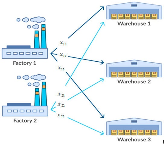
Figure 1. The transportation problem.

Table 1. Transportation problem tableau.

	Demand	WHS 1	WHS 2	WHS 3	Supply
Supply
FAC 1		${\lambda }_1{x}_{11}$	$2x_{12}$	$7x_{13}$$7x_{13}$	13
		$x_{11}$	$x_{12}$	$x_{13}$
FAC 2		${\lambda }_2{x}_{21}$	$9x_{22}$	$3x_{23}$	15
		$x_{21}$	$x_{22}$	$x_{23}$
Demand		11	3	14	28

Step (0).

For certain $\upsilon =(13,15)$ the problem $P(\lambda ,\upsilon )$ is transformed to $P(\lambda )$

$$\begin{array}{c}P(\lambda )\hfill \\ Min F={\lambda }_1{x}_{11}^2+2x_{12}^2+7x_{13}^2+{\lambda }_2{x}_{21}^2+9x_{22}^2+3x_{23}^2\hfill \\ s.t.: x_{11}+x_{12}+x_{13}\le 13,\hfill \\ x_{21}+x_{22}+x_{23}\le 15,\\ x_{11}+x_{21}=11,\\ x_{12}+x_{22}=3,\\ x_{13}+x_{23}=14,\\ x_{ij}\ge 0\end{array}$$

Step (1).

the optimal solution is

$$x_{11}=11,{ \mathrm{x}}_{12}=0,{ \mathrm{x}}_{21}=0,{ \mathrm{x}}_{22}=3,{ \mathrm{x}}_{13}=2,{ \mathrm{x}}_{23}=12,{ \mathrm{F}}^{*}=622 \mathrm{With} {\lambda }^{*}=(1,1)$$

Step (2).

the desired feasible solution is

$$\begin{array}{l}{x}^{\circ }=(x_{11},{ \mathrm{x}}_{12},{\mathrm{x}}_{21},{\mathrm{x}}_{22},{ \mathrm{x}}_{13},{\mathrm{x}}_{23})\\ x_{11}=11,{ \mathrm{x}}_{12}=2,{ \mathrm{x}}_{21}=0,{ \mathrm{x}}_{22}=1,{ \mathrm{x}}_{13}=0,{ \mathrm{x}}_{23}=14\end{array}$$

Step (3).

Formulate the K.K.T conditions to get the domain of $\lambda$ such that $x^{\circ }$ is optimal one

$$\begin{array}{l}2{\lambda }_1{x}_{11}+u_1+v_1=0\\ 4x_{11}+u_1+v_2=0\\ 14x_{13}+u_1+v_3=0\\ 2{\lambda }_2{x}_{21}+u_2+v_1=0\\ 18x_{22}+u_2+v_2=0\\ 9x_{23}+u_2+v_3=0\\ u_1(x_{11}+x_{12}+x_{13}-13)=0\\ u_2(x_{21}+x_{22}+x_{23}-15)=0\\ u_1,u_2\ge 0,{ \mathrm{v}}_1,v_2,v_3\ne 0\end{array}$$

By Substituting with $x^{\circ }$ we get

$$D(\lambda )=\{({\lambda }_1,{\lambda }_2)\in R^2|{\lambda }_1-10\ge 0,{\lambda }_2-14\ge 0\}$$

Step (4).

Formulate $D(\lambda )$ to find the of values ${\lambda }_1,{\lambda }_2$

$$\begin{array}{l}\min \Vert \lambda -{\lambda }^{*}\Vert \\ s.t.\lambda \in D(\lambda )\end{array}$$

For $L_2$ norm

$$\begin{array}{l}\min \Vert \lambda -{\lambda }^{*}\Vert =\min \sqrt{{({\lambda }_1-1)}^2+{({\lambda }_2-1)}^2}\\ s.t.\lambda \in D(\lambda )\end{array}$$

Solving this NLP using “LINDO” software we get ${\lambda }_1=10, {\lambda }_2=14,$ then ${\lambda }^{\circ }=(10,14)$

Phase 2:

Formulate parametric inverse nonlinear transportation problem

Substituting by ${\lambda }^{\circ }=(10,14)$, letting us form the parametric P(u) problem: parameters in the constraints as follows:

$$\begin{array}{c}P(\upsilon ):\hfill \\ Min F=10x_{11}^2+2x_{12}^2+7x_{13}^2+14x_{21}^2+9x_{22}^2+3x_{23}^2\hfill \\ s.t.: x_{11}+x_{12}+x_{13}\le {\upsilon }_1,\hfill \\ x_{21}+x_{22}+x_{23}\le {\upsilon }_2,\\ x_{11}+x_{21}=11,\\ x_{12}+x_{22}=3,\\ x_{13}+x_{23}=14,\\ x_{ij}\ge 0\end{array}$$

Phase 3:

Stability analysis

Construct the K.K.T of $P(\upsilon )$ with optimal solution

$$\begin{array}{l}{x}^{\circ }=(x_{11},{ \mathrm{x}}_{12},{\mathrm{x}}_{21},{\mathrm{x}}_{22},{ \mathrm{x}}_{13},{\mathrm{x}}_{23})\\ x_{11}=11,{ \mathrm{x}}_{12}=2,{ \mathrm{x}}_{21}=0,{ \mathrm{x}}_{22}=1,{ \mathrm{x}}_{13}=0,{ \mathrm{x}}_{23}=14\end{array}$$

and ${\lambda }^{\circ }=(10,14)$ to be as follows:

$$\begin{array}{l}24x_{11}+u_1+v_1=0\\ 4x_{12}+u_1+v_2=0\\ 14x_{13}+u_{{}_1}+v_3=0\\ 28x_{21}+u_2+v_1=0\\ 18x_{22}+u_2+v_2=0\\ 9x_{23}+u_2+v_3=0\\ u_1(x_{11}+x_{12}+x_{13}-v_1)=0\\ u_2(x_{21}+x_{22}+x_{23}-v_2)=0\\ u_1,u_2\ge 0\\ v_1,v_2,v_3\ne 0\end{array}$$

At $x^{\circ }$,

$$\begin{array}{l}264+u_1+v_1=0\\ 8+u_1+v_2=0\\ u_1+v_3=0\\ u_2+v_1=0\\ 36+u_2+v_2=0\\ 126+u_2+v_3=0\\ u_1(11+2+0-v_1)=0\\ u_2(0+1+14-v_2)=0\\ u_1,u_2\ge 0\\ v_1,v_2,v_3\ne 0\end{array}$$

It is clear that $u_1,u_2\ne 0$ then we get the stability set of the first type at $x^{\circ }$ as follows

$$G(12,14)=\{v\in R^2|13-v_1=0,12-v_2=0\}$$

It is clear that, for this application, we not only justify the cost function parameters as little as possible so that the specific feasible solution ($x_{11}=11,{ \mathrm{x}}_{12}=2,{\mathrm{x}}_{21}=0,{\mathrm{x}}_{22}=1,{ \mathrm{x}}_{13}=0,{\mathrm{x}}_{23}=14$) becomes an optimal one but also, a solution stability set of parameters was investigated to keep the new optimal solution is unchanged.

7. Conclusions

The inverse optimization problem is an interesting field for both academic scientist and real-life applications. Implementation the inverse optimization and adapting the cost function parameters as little as possible so that the specific feasible solution becomes an optimal spatially in nonlinear domain is not easy, so keeping that solution with different sets of certain parameters is valuable. Nonlinear transportation problem (NTP) is a special case of nonlinear programming problem (NLP), the formulation of the NTP is more specific, especially in terms of decision variables and the set of constraints.

This manuscript proposed a methodology for finding the inverse problem of convex nonlinear programming problem $P(\lambda ,\upsilon )$ having tuning parameters $\lambda \in R^m$ in the function of the objective and input parameters $\upsilon \in R^l$ in the functions in the set of constraint. The proposed method consists of three phases. Firstly, based on the optimality conditions, tuning parameters $\lambda \in R^m$ are tuned as less as possible so that the given initial feasible solution $x^o$ becomes the optimal ones. Secondly, using input parameters, $\upsilon \in R^l$ the resulting problem is reformulated in parametric form $P(\upsilon )$. Then, based on the stability notions, the availability domain of the input parameters was detected to keep its optimal solution unchanged.

Finally, to validate and demonstrate the advantage of the new approach, three nonlinear programming examples and nonlinear transportation problem application are provided for the sake of illustration. On solving the transportation problem by the given approach, we summarize the result as follows:

When the input parameters $\upsilon =(13,15)$ and the tuning parameters ${\lambda }^{*}=(1,1)$ the optimal solution was $x_{11}=11,{ \mathrm{x}}_{12}=0,{ \mathrm{x}}_{21}=0,{ \mathrm{x}}_{22}=3,{ \mathrm{x}}_{13}=2,{ \mathrm{x}}_{23}=12$, but the decision making need that the solution $x_{11}=11,{ \mathrm{x}}_{12}=2,{ \mathrm{x}}_{21}=0,{ \mathrm{x}}_{22}=1,{ \mathrm{x}}_{13}=0,{ \mathrm{x}}_{23}=14$ to be an optimal one, this methodology not only achieve the goal but also detect the stability set of the first type, which is used to define a available range of these input parameters $G(12,14)=\{v\in R^2|13-v_1=0,12-v_2=0\}$ that keep the solution $x_{11}=11,{ \mathrm{x}}_{12}=2,{ \mathrm{x}}_{21}=0,{ \mathrm{x}}_{22}=1,{ \mathrm{x}}_{13}=0,{ \mathrm{x}}_{23}=14$ as an optimal one. From the above study, the following may be concluded:

• A solution of a parametric inverse transportation problem is introduced.
• The paper deals with Parametric nonlinear programming having tuning parameters $\lambda \in R^m$ in the objective and input parameters $\upsilon \in R^l$ in the constraints.
• An inverse model for the proposed problem was investigated.
• Solution stability of the problem was investigated to retain its optimal solution.
• Numerical examples are provided for the sake of illustration.

For the future work, this method can be extended to nonlinear Large-Scale Inverse transportation Problems and its applications in IoT.

References

- Ghobadi, K.; Lee, T.; Mahmoudzadeh, H.; Terekhov, D. Robust inverse optimization. Oper. Res. Lett. 2018, 46, 339–344. [Google Scholar] [CrossRef]
- Babier, A.; Chan, T.C.; Lee, T.; Mahmood, R.; Terekhov, D. A unified framework for model fitting and evaluation in inverse linear optimization. arXiv 2019, arXiv:1804.04576. [Google Scholar]
- Chan, T.C.; Kaw, N. Inverse optimization for the recovery of constraint parameters. Eur. J. Oper. Res. 2020, 282, 415–427. [Google Scholar] [CrossRef]
- Chow, J.Y.; Ritchie, S.G.; Jeong, K. Nonlinear inverse optimization for parameter estimation of commodity-vehicle-decoupled freight assignment. Transp. Res. Part E Logist. Transp. Rev. 2014, 67, 71–91. [Google Scholar] [CrossRef]
- Burton, D.; Toint, P.L. On an instance of the inverse shortest paths problem. Math. Program. 1992, 53, 45–61. [Google Scholar] [CrossRef]
- Xu, S.; Zhang, J. An inverse problem of the weighted shortest path problem. Jpn. J. Ind. Appl. Math. 1995, 12, 47–59. [Google Scholar] [CrossRef]
- Zhang, J.; Liu, Z.; Ma, Z. On the inverse problem of minimum spanning tree with partition constraints. Math. Methods Oper. Res. 1996, 44, 171–187. [Google Scholar] [CrossRef]
- Zhang, J.; Liu, Z. A general model of some inverse optimization problems and its solution method under l8 norm. J. Comb. Optim. 2002, 6, 207–227. [Google Scholar] [CrossRef]
- Ahuja, R.K.; Orlin, J.B. Inverse Optimization. Oper. Res. 2001, 49, 771–783. [Google Scholar] [CrossRef]
- Zhang, J.; Liu, Z. Calculating some inverse linear programming problems. J. Comput. Appl. Math. 1996, 72, 261–273. [Google Scholar] [CrossRef]
- Zhang, J.; Liu, Z. A further study on inverse linear programming problems. J. Comput. Appl. Math. 1999, 106, 345–359. [Google Scholar] [CrossRef]
- Huang, S.; Liu, Z. On the inverse problem of linear programming and its application to minimum weight perfect k-matching. Eur. J. Oper. Res. 1999, 112, 421–426. [Google Scholar] [CrossRef]
- Amin, G.R.; Emrouznejad, A. Inverse forecasting: A new approach for predictive modeling. Comput. Ind. Eng. 2007, 53, 491–498. [Google Scholar] [CrossRef]
- Zhang, J.; Zhang, L.-W.; Xiao, X. A Perturbation approach for an inverse quadratic programming problem. Math. Methods Oper. Res. 2010, 72, 379–404. [Google Scholar] [CrossRef]
- Jiang, Y.; Xiao, X.; Zhang, L.; Zhang, J. A perturbation approach for a type of inverse linear programming problems. Int. J. Comput. Math. 2011, 88, 508–516. [Google Scholar] [CrossRef]
- Scheafer, A.J. Inverse integer programming. Opt. Lett. 2009, 3, 483–489. [Google Scholar] [CrossRef]
- Wang, L. Cutting plane algorithms for the inverse mixed integer linear programming problem. Oper. Res. Lett. 2009, 37, 114–116. [Google Scholar] [CrossRef]
- Osman, M.S.A. Qualitative Analysis of Basic Notions in Parametric Convex Programming II: Parameters in the Objective Function. Aplikace Matematiky 1997, 22, 333–348. [Google Scholar] [CrossRef]
- Osman, M.S.A.; EL-Hefni, M.R. Determination of the Stability Sets in Parametric Convex Programming Problems. In Proceedings of the Second Conference on Operations Research and its Military Applications, Military Technical College (M.T.C.), Cairo, Egypt, 17–19 November 1987. [Google Scholar]
- Osman, M.S.A.; El-Hefny, M.R.; El-Ariny, A.K.H. Implementing stability results in solving large scale convex programming problems. In Analysis and Optimization of Systems. Lecture Notes in Control and Information Sciences; Bensoussan, A., Lions, J.L., Eds.; Springer: Berlin/Heidelberg, Germany, 1988; Volume 111, pp. 543–556. [Google Scholar]
- Mathur, N.; Srivastava, P.K.; Paul, A. Algorithms for solving fuzzy transportation problem. Int. J. Math. Oper. Res. 2018, 12, 190. [Google Scholar] [CrossRef]
- Xu, S.J.; Nourinejad, M.; Lai, X.; Chow, J.Y. Network Learning via Multiagent Inverse Transportation Problems. Transp. Sci. 2018, 52, 1347–1364. [Google Scholar] [CrossRef]
- Jain, S.J.S. An Inverse Capacitated Transportation Problem. IOSR J. Math. 2013, 5, 24–27. [Google Scholar] [CrossRef]
- Stuart, A.M.; Wolfram, M.-T. Inverse Optimal Transport. SIAM J. Appl. Math. 2020, 80, 599–619. [Google Scholar] [CrossRef]
- Nguyan, T.D. Applictions of Robust and Inverse Optimization in Transportation. Master’s Thesis, Massachusetts Institute of Technology, Cambridge, MA, USA, September 2010. [Google Scholar]
- Sanjay, J. An Inverse Transportation Problem with the Linear Fractional Objective Function. AMO Adv. Model. Optim. 2013, 15, 677–678. [Google Scholar]
- Yang, D.; Gao, D. Study on Some Kinds of the Inverse Transportation Problems. In Proceedings of the Eighth International Conference of Chinese Logistics and Transportation Professionals (ICCLTP), Chengdu, China, 8–10 October 2008. [Google Scholar]
- Abo-Elnaga, Y.; Mousa, A.A. Inverse optimization for nonlinear programming problems. Wulfenia J. 2014, 21, 307–317. [Google Scholar]
- Bazaraa, M.S.; Sherali, H.D.; Shetty, C.M. Nonlinear Programming: Theory and Algorithms, 3rd ed.; Wiley: Hoboken, NJ, USA, 2006. [Google Scholar]
Publisher’s Note: MDPI stays neutral with regard to jurisdictional claims in published maps and institutional affiliations. |
© 2020 by the authors. Licensee MDPI, Basel, Switzerland. This article is an open access article distributed under the terms and conditions of the Creative Commons Attribution (CC BY) license (http://creativecommons.org/licenses/by/4.0/).