Abstract
A new method of numerical integration for a perturbed and damped systems of linear second-order differential equations is presented. This new method, under certain conditions, integrates, without truncation error, the IVPs (initial value problems) of the type: , , , , which appear in structural dynamics, astrodynamics, and other fields of physics and engineering. In this article, a succession of real functions is constructed with values in the algebra of matrices. Their properties are studied and we express the solution of the proposed IVP through a serial expansion of the same, whose coefficients are calculated by means of recurrences involving the perturbation function. This expression of the solution is used for the construction of the new numerical method. Three problems are solved by means of the new series method; we contrast the results obtained with the exact solution of the problem and with its first integral. In the first problem, a quasi-periodic orbit is integrated; in the second, a problem of structural dynamics associated with an earthquake is studied; in the third, an equatorial satellite problem when the perturbation comes from zonal harmonics is solved. The good behavior of the series method is shown by comparing the results obtained against other integrators.
1. Introduction
Many problems of physics and engineering are modeled by perturbed and damped differential equations systems of the second order: , , , .
These systems, known in structural dynamics as two-degree of freedom (2DOF) systems, are used to evaluate the motion of a structure with an attached control system. The dynamic response of structures is interesting for the study of earthquakes.
These 2DOF systems also appear when attempting to reduce the vibration amplitude of a single degree of freedom (SDOF) system, subjected to harmonic excitation when it is connected to a tuned vibration absorber [1,2,3,4,5,6,7].
In celestial mechanics, models such as the classic two-body problem and the satellite problem are reduced to a system of oscillators of this type through the transformations of Kunstaanheimo–Stiefel [8] or Burdet–Ferrándiz [9,10].
The Runge–Kutta type methods [11,12,13,14,15,16,17,18] that usually solve these second-order systems require a large number of evaluations of the perturbation function. This is an inconvenience for its implementation on a computer. Other methods for solving second-order systems can be found in Saravi [19].
Different ideas and motivations led several authors to develop special methods for the integration of oscillatory problems. Among the algorithms designed specifically for the numerical resolution of second-order systems are Falkner methods, the Adams extrapolation formulas, Störner–Cowell methods [20,21], and Gauss–Jackson methods [22,23]. Scheifele [24], Stiefel and Scheifele [25], Stiefel and Bettis [26], and Bettis [27,28], followed by Martín and Ferrándiz [29,30,31], Martín and Farto [32], You et al. [33], Vigo–Aguiar and Ferrándiz [34], Reyes et al. [35], and García-Alonso et al. [36], among others, developed numerical methods for the integration of systems of first-order perturbed linear differential equations. These methods can precisely integrate the unperturbed problem. M. Ruggieri and M. P. Speciale [37] carried out a study on perturbed systems of partial differential equations (PDEs) for viscoelastic media, and in some cases, the authors computed approximate solutions by means of the approximate generator of the first-order approximate group of transformations.
This article presents a series method that retains this property and allows for the precise numerical integration of perturbed and damped linear differential systems of the second order. The new method, under certain conditions, will accurately integrate the perturbed and damped problem. The integration is carried out without any previous transformation of the proposed system.
Moreover, this series method is the basis for the construction of multistep explicit, implicit, and predictor–corrector numerical methods.
To this end, a linear operator will be applied to the system of differential equations, where D is a differential operator defined as , and B is an appropriate matrix chosen to be able to annul the perturbation function. A family of real functions, , will be defined with values in , with which a series method will be constructed. This series method will integrate exactly, with only the first three functions, an unperturbed system of the third-order equivalent to the given one.
Finally, three problems are solved herein by the method of the functions series; we contrast the results obtained with the exact solution of the problem and with its first integral. The first example is the integration of a quasi-periodic orbit [38,39,40,41]. The second one is a structural dynamics problem associated with an earthquake [6,7], and the third one studies an equatorial satellite with perturbation [10,29,42,43].
The good performance of the series method is evidenced by the comparison of the results obtained against other well-known integrators, such as LSODE, ROSENBROCK, GEAR, and DVERK78.
2. Formulation of the Problem
The IVP to be considered is
where , , is a perturbation parameter, usually small, and .
The components of the vector perturbation field are with , and the field is continuous, with continuous derivatives until a certain order satisfies the conditions for the existence and uniqueness of the solution.
This type of system is called a perturbed and damped linear system of the second order.
It is considered that is an analytical function in I with respect to t. Designating and , it is possible to write
The IVP (1) can be written using the linear operator derivation :
Let us make ; if is applied in (3), it obtains the IVP:
where the initial values are
which has the exact same solution as (1) and (3).
By defining , if , , and , can be written as .
Henceforth, the IVP (4) is
The idea that leads to considering (5) is to eliminate the perturbation with the operator.
3. The Functions
For the construction of the functions, the following IVP is considered:
where , with and being the identity matrix and the zero matrix of this algebra, respectively.
Definition 1.
The functions, which verify with , will be called Ψ functions.
Therefore, the functions are the functions, solutions of the following IVPs:
Proposition 1.
The Ψ functions verify the following:
Proof.
Of the initial three conditions . The one that requires a justification is the third, which is obtained from (8). The other two are evident by the definition.
Since and verify the same IVP, by the existence and uniqueness theorem of solutions, it can be said that with . □
Proposition 2.
The Ψ functions verify the following recurrent relation:
Proof.
is replaced with in (8). □
Definition 2.
, , and are the solutions of the following unperturbed system:
with the initial conditions:
respectively.
can be also calculated as exponential functions of a particular matrix.
In the case , the IVP is considered:
with the following initial conditions:
where .
Equation (17) can be expressed as follows:
We will call the submatrix formed by the first rows and the m columns of .
In the case where , the following IVP must be taken into consideration:
with the following initial conditions:
where .
The submatrix formed by the to rows and the first m columns of is denoted by .
Similarly, the calculation of defines
and considers the following system:
whose solution is
The submatrix formed by the to rows and the first m columns of is denoted by .
Proposition 3.
.
Proof.
The initial conditions and are according to the definition of the functions. The third initial condition is achieved from (8):
Since and verify the same IVP, by the existence and uniqueness theorem of solutions, we can say that . □
Proposition 3 extends Proposition 1 to and Proposition 2 to .
Theorem 1.
The IVP
has the following solution:
Proof.
Taking into account Definition 2 and the linearity of the operator , the following is obtained:
Definition 2 is enough to demonstrate the following initial conditions:
□
Theorem 2.
The solution of the IVP (6) is
Proof.
It is required to prove that verifies the following:
For the operator’s linearity and Theorem 1, it is necessary to have
and Definitions 1 and 2 are enough to the demonstrate the following initial conditions:
□
4. A New Series Method
In this section, a new numerical series method is shown, based on the functions, by truncating the solution exposed in Theorem 2.
Through expressing the solution of the IVP (1) in the power series
by substituting the McLaurin expansion (34) in (1), we obtain
Therefore, recurrences can be achieved between the and :
The solution can then be expressed as
In (40), in addition to a more compact notation than in (37), the coefficients of the series depend only on .
Once the coefficients from are calculated, with step size h, the approximation to the solution of (5) at a point is given by
Once the approximation of the solution and its derivatives at a point , which are noted as , , and , are calculated, verifying
to obtain an approximation to the solution at a point , a change to the independent variable is made, so
which leads to the initial situation.
Considering
the approximation to the solution at a point is
Residue Calculation
The exact solution of IVP (5) is
Carrying out a truncation of functions, with ,
Since
the corresponding residue is given by
Therefore, the perturbation parameter is a common factor of the truncation error. If , that is, if the perturbation disappears in an arbitrary instant of the independent variable t, the functions series method integrates the IVP (5) without the truncation error.
5. Applications for the Functions Series Method
An implementation of this algorithm is used to approximate the solution of certain IVPs, modeled by second-order systems of differential equations, proposed by various authors.
The results obtained by well-known methods and the functions series method, versus the analytical solution of the IVP, show the good behavior of the new series method based in functions.
5.1. Problem 1
This problem presents an application of the method to a test problem presented in [25], which can also be found in [26,38,39,40,41], among others.
Let us consider the following IVP:
The problem is solved as a pair of uncoupled equations. Denoting and by substituting in (50), we get the following second-order system:
for which the analytical solution is
The solution represents the motion on a perturbation of a circular orbit in the complex plane.
We express (51) as
The matrix that annihilates the perturbation function is . Applying the operator to the system (53) results in
The integration with , , and is achieved with the following algorithm:
From up to n, the following is calculated:
following k.
Figure 1 shows the graph of the logarithm of the relative error module of the solution , calculated by means of (45) with three functions, step size , and 50 digits. This result is compared to the numerical integration algorithms: DEVERK78 with a tolerance of , GEAR with errorper = Float(1,−30), LSODE[backfunc] with a tolerance of , and ROSENBROCK with abserr = Float(1,−30).
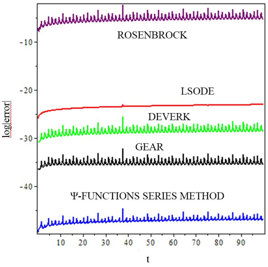
Figure 1.
The module’s decimal logarithm of the relative error of the equatorial satellite position.
5.2. Problem 2
In this problem (2DOF) [6,7], the structure of Figure 2 is solved. This structure is submitted to seismic movement in which only horizontal displacement is considered.
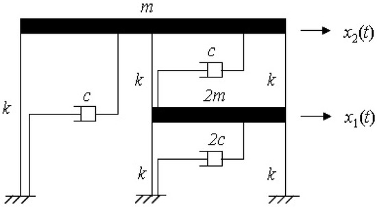
Figure 2.
Two-story frame.
and is defined as the relative displacement between the mass and the ground, where and are the absolute displacements of the masses, and and are the absolute ground displacement and the absolute ground velocity, respectively.
The equation of motion for the system is
where m is the mass, c is the damping coefficient, and k is the stiffness coefficient.
If is an harmonic matrix forcing function, i.e.,
where is the frequency of the disturbance, then the Equation (56) is
Normalizing the Equation (58), the following is obtained:
At the initial moment that the seismic movement occurs, it is logical to assume that the structure is at rest, i.e., , , and .
Following Steffensen’s techniques [44,45], a new variable is added: .
This variable allows us to eliminate the perturbation function of the IVP (59), obtaining a new IVP:
The matrix eliminates the disturbance function. Applying the operator to the system (60) results in
which is solved by the next algorithm, with , , , and . The frequency of the disturbance function is equal to the natural frequency of vibration of the following structure:
From up to n, the following is calculated:
following k.
Figure 3 shows the graph of the module’s decimal logarithm of the relative error of the relative displacement between the mass and the ground , calculated by means of (45) with three functions, a step size of , and 50 digits. This result is compared to the numerical integration algorithms: DEVERK78 with a tolerance of , GEAR with errorper = Float(1,−30), LSODE[backfunc] with a tolerance of , and ROSENBROCK with abserr = Float(1,−30).
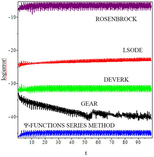
Figure 3.
The module’s decimal logarithm of the relative error of the relative displacement between the mass and the ground.
5.3. Problem 3
In this case, the method is applied to the numerical calculus of the position of an Earth artificial satellite with periodic equatorial orbit that is affected by the perturbation of the zonal harmonic [30,42].
This problem, expressed by the Burdet–Ferrándiz variables (B–F) [10,43], can be formulated by perturbed and decupled oscillators with unit frequency.
The B–F coordinates are the direction cosines and the inverse of the satellite radius using, as an independent variable, the “true anomaly,” u. The angular momentum, c, can be considered as a constant, the reduced mass is , and the orbit eccentricity is e.
with the following initial conditions:
Making the change of variable , we can rewrite (63) in the following form:
This is integrated by means of the following algorithm:
A serious drawback occurs in the case of very eccentric orbits since the speed of the satellite in perigee is great, and this circumstance, together with the strong curvature of the trajectory, can cause a loss of precision in integration.
Orbits with zero eccentricity and high eccentricity are considered, respectively:
- for : , ;
- for : , .
Figure 4 and Figure 5 show the graph of the logarithm of the relative error module of the solution , calculated by means of (45), a step size of , and 50 digits. This result is compared to the numerical integration algorithms: DEVERK78 with a tolerance of , GEAR with errorper = Float(1,−30), LSODE[backfunc] with a tolerance of , and ROSENBROCK with abserr = Float(1,−30).
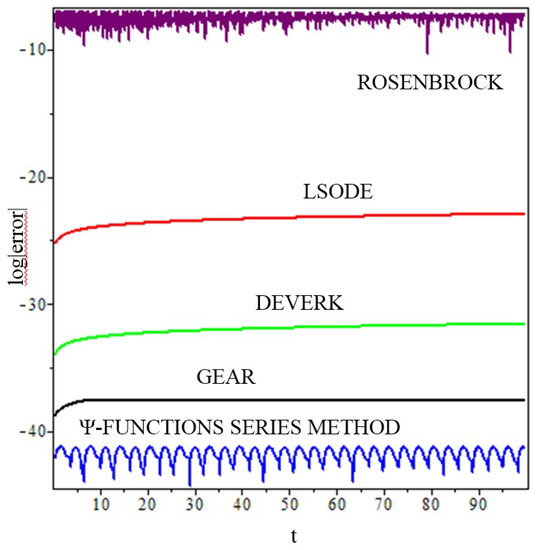
Figure 4.
Trajectory error of a circular equatorial -perturbed satellite orbit, integrated with twenty functions and .

Figure 5.
Trajectory error of an equatorial -perturbed satellite orbit, integrated with twenty functions and .
6. Conclusions
A family of analytical functions, the functions, has been defined by studying their properties. Based on these functions and under certain hypotheses, a series method has been constructed that allows, without truncation error, the numerical integration of a wide range of problems modeled by means of systems of second-order differential equations, forced and damped. The function series method exactly integrates the unperturbed and damped problem when it is possible to cancel the perturbation function by means of a differential operator.
This method has the advantage, compared to other known integrators, of being able to transform a second-order forced and damped problem into an undisturbed problem that integrates in a precise manner, by applying a differential operator.
The integration is carried out without any previous transformation of the proposed system. This series method is the basis for the construction of multistep explicit, implicit, and predictor-corrector numerical methods.
The good behavior of the functions series method was shown in the following three problems we solved, contrasting the exact solution or the first integral with this method and other known integrators implemented in MAPLE (Deverk78, Gear, Lsode, and Rosenbrock):
- The integration of a quasi-periodic orbit—in contrast, the exact solution of the problem is used;
- A problem of structural dynamics associated with an earthquake—the analytical solution of the problem was used for comparison;
- An equatorial satellite with perturbation , with high and low eccentricity—the process of contrast was carried out using a first integral.
Author Contributions
Conceptualization, F.G.-A. and J.A.R.; methodology, F.G.-A. and J.A.R.; software, F.G.-A., J.A.R., and M.C.-M.; validation, F.G.-A., J.A.R., and M.C.-M.; formal analysis, F.G.-A., J.A.R., and M.C.-M.; investigation, F.G.-A., J.A.R., and M.C.-M.; data curation, F.G.-A., and J.A.R.; writing—original draft preparation, F.G.-A., J.A.R., and M.C.-M.; writing—review and editing, F.G.-A., J.A.R., and M.C.-M.; supervision, F.G.-A. and J.A.R.; project administration, F.G.-A.; funding acquisition, J.A.R. All authors have read and agreed to the published version of the manuscript.
Funding
This research received no external funding.
Conflicts of Interest
The authors declare that there is no conflict of interest.
References
- Newmark, N.M. A method of computation for structural dynamics. ASCE J. Eng. Mech. Div. 1959, 85, 67–94. [Google Scholar]
- Chung, J.; Hulbert, G.M. A family of single-step Houbolt time integration algorithms for structural dynamics. Comput. Methods Appl. Mech. Eng. 1994, 118, 1–11. [Google Scholar] [CrossRef][Green Version]
- Craig, R.R., Jr.; Kurdila, A.J. Fundamentals of Structural Dynamics; John Wiley and Sons Inc.: Hoboken, NJ, USA, 2006. [Google Scholar]
- Chopra, A.K. Dynamics of Structures: Theory and Applications to Earthquake Engineering, 3rd ed.; Prentice-Hall: Upper Saddle River, NJ, USA, 2007. [Google Scholar]
- Gholampour, A.; Ghassemieh, M. New implicit method for analysis of problems in nonlinear structural dynamics. Appl. Comput. Mech. 2011, 5, 15–20. [Google Scholar]
- Hart, G.C.; Wong, K. Structural Dynamics for Structural Engineers; John Wiley & Sons, Inc.: Hoboken, NJ, USA, 1999. [Google Scholar]
- Bangash, M.Y.H. Analyses, Numerical Computations, Codified Methods; Springer: Berlin/Heidelberg, Germany, 2011. [Google Scholar]
- Kunstaanheimo, P.; Stiefel, E. Perturbation theory of Kepler motion based on spinor Regularization. J. Reine Angew. Math. 1965, 218, 204–219. [Google Scholar] [CrossRef]
- Burdet, C.A. Le mouvement Keplerian et les oscillateurs harmoniques. J. Reine Angew. Math. 1969, 238, 71–78. [Google Scholar] [CrossRef]
- Ferrándiz, J.M. A general canonical transformation increasing the number of variables with application to the two-body problem. Celest. Mech. 1988, 41, 343–357. [Google Scholar]
- Simos, T.E. A phase-fitted Runge-Kutta-Nyström methods for the numerical solution of initial value problems with oscillating solutions. Comput. Phys. Commun. 2009, 180, 1839–1846. [Google Scholar]
- Yang, H.; Wu, X.; You, X.; Fang, Y. Extended RKN-type methods for numerical integration of perturbed oscillators. Comput. Phys. Commun. 2009, 180, 1777–1794. [Google Scholar] [CrossRef]
- Yang, H.; Zeng, X.; Wu, X.; Ru, Z. A Simplified Nystrom-Tree Theory for Extended Runge-Kutta-Nystrom Integrators Solving. Comput. Phys. Commun. 2014, 185, 2841–2850. [Google Scholar] [CrossRef]
- González, A.B.; Farto, J.M.; López, D.J. Reformulation of the RKGM Methods using Scheifele Expansions. Appl. Math. Lett. 2000, 13, 63–66. [Google Scholar] [CrossRef][Green Version]
- Fang, Y.; Wu, X. A New Pair of Explicit ARKN Methods for the Numerical Integration of General Perturbed Oscillators. Appl. Numer. Math. 2007, 57, 166–175. [Google Scholar] [CrossRef]
- You, X.; Zhao, J.; Yang, H.; Fang, Y.; Wu, X. Order Conditions for RKN Methods Solving General Second-Order Oscillatory Systems. Numer. Algorithms 2014, 66, 147–176. [Google Scholar] [CrossRef]
- Martín, P.; López, D.J.; García, A. Implementation of Falkner method for problems of the form y” = f(x,y). Appl. Math. Comput. 2000, 109, 183–187. [Google Scholar] [CrossRef]
- Franco, J.M. New Methods for Oscillatory Systems Based on ARKN Methods. Appl. Numer. Math. 2006, 56, 1040–1053. [Google Scholar] [CrossRef]
- Saravi, M. A procedure for solving some second-order linear ordinary differential equations. Appl. Math. Lett. 2012, 25, 408–411. [Google Scholar] [CrossRef]
- Dormand, J.R. Numerical Methods for Differential Equations. A Computational Approach; CRC Press: Boca Ratón, FL, USA, 1996. [Google Scholar]
- Henrici, P. Discrete Variable Methods in Ordinary Differential Equations; John Wiley & Sons: New York, NY, USA, 1962. [Google Scholar]
- Herrick, S. Astrodynamics. Vol. 2: Orbit Correction, Perturbation Theory Integration; Van Nostrand Reinhold: London, UK, 1972. [Google Scholar]
- González, A.B.; Martín, P. A note concerning Gauss-Jackson method. Extr. Math. 1996, 11, 255–260. [Google Scholar]
- Scheifele, G. On Numerical Integration of Perturbed Linear Oscillating Systems. ZAMP 1971, 22, 186–210. [Google Scholar] [CrossRef]
- Stiefel, E.L.; Scheifele, G. Linear and Regular Celestial Mechanics; Springer: New York, NY, USA, 1971. [Google Scholar]
- Stiefel, E.; Bettis, D.G. Stabilization of Cowell’s Method. Numer. Math. 1969, 13, 154–175. [Google Scholar] [CrossRef]
- Bettis, D.G. Stabilization of finite difference methods of numerical integration. Celest. Mech. 1970, 2, 282–295. [Google Scholar] [CrossRef]
- Bettis, D.G. Numerical integration of products of Fourier and ordinary polinomials. Numer. Math. 1970, 14, 421–434. [Google Scholar] [CrossRef]
- Martín, P.; Ferrándiz, J.M. Behaviour of the SMF method for the numerical integration of satellite orbits. Celest. Mech. Dyn. Astron. 1995, 63, 29–40. [Google Scholar] [CrossRef]
- Martín, P.; Ferrándiz, J.M. Multistep numerical methods based on Scheifele G-functions with application to satellite dynamics. SIAM J. Numer. Anal. 1997, 34, 359–375. [Google Scholar] [CrossRef]
- Martín, P.; Ferrándiz, J.M. Numerical integration of perturbed linear systems. Appl. Math. 1999, 31, 183–189. [Google Scholar] [CrossRef]
- Martín, P.; Farto, J.M. Increasing the order of the SMF method for a special type of problem. SIAM J. Numer. Anal. 1998, 35, 773–777. [Google Scholar] [CrossRef]
- You, X.; Zhang, Y.; Zhao, J. Trigonometrically-Fitted Scheifele Two-Step. Methods for Perturbed Oscillators. Comput. Phys. Commun. 2011, 182, 1481–1490. [Google Scholar] [CrossRef]
- Vigo-Aguiar, J.; Ferrándiz, J.M. Higher-order variable-step algorithms adapted to the accurate numerical integration of perturbed oscillators. Comput. Phys. 1998, 12, 467–470. [Google Scholar] [CrossRef]
- Reyes, J.A.; García-Alonso, F.; Ferrándiz, J.M.; Vigo-Aguiar, J. Numeric multistep variable methods for perturbed linear system integration. Appl. Math. Comput. 2007, 190, 63–79. [Google Scholar] [CrossRef]
- García-Alonso, F.; Reyes, J.A. A new approach for exact integration of some perturbed stiff linear systems of oscillatory type. Appl. Math. Comput. 2009, 215, 2649–2662. [Google Scholar]
- Ruggieri, M.; Speciale, M.P. Approximate Analysis of Nonlinear Dissipative Model. Acta Appl. Math. 2014, 132, 549–559. [Google Scholar] [CrossRef]
- Vigo-Aguiar, J.; Ferrándiz, J.M. A general procedure for the adaptation of multistep algorithms to the integration of oscillatory problems. SIAM J. Numer. Anal. 1998, 35, 1684–1708. [Google Scholar] [CrossRef]
- Simos, T.E.; Vigo-Aguiar, J. Exponentially fitted sympletic integrator. Phys. Rev. E 2003, 67, 1–7. [Google Scholar] [CrossRef] [PubMed]
- Ramos, J.I. Piecewise-linearized methods for initial-value problems with oscillating solutions. Appl. Math. Comput. 2006, 181, 123–146. [Google Scholar] [CrossRef]
- Van de Vyver, H. Two-step hybrid methods adapted to the numerical integration of perturbed oscillators. arXiv 2006, arXiv:math/0612637v1. [Google Scholar]
- Janin, G. Accurate computation of highly eccentric satellite orbits. Celest. Mech. 1974, 10, 451–456. [Google Scholar] [CrossRef]
- Ferrándiz, J.M.; Sansaturio, M.E.; Pojman, J.R. Increased accuracy of computations in the main satellite problem through linearization methods. Celest. Mech. 1992, 53, 347–364. [Google Scholar] [CrossRef]
- Steffensen, J.F. On the Differential Equations of Hill in the Theory of the Motion of the Moon. Acta Math. 1955, 93, 169–177. [Google Scholar] [CrossRef]
- Steffensen, J.F. On the Differential Equations of Hill in the Theory of the Motion of the Moon (II). Acta Math. 1955, 95, 25–37. [Google Scholar] [CrossRef]
Publisher’s Note: MDPI stays neutral with regard to jurisdictional claims in published maps and institutional affiliations. |
© 2020 by the authors. Licensee MDPI, Basel, Switzerland. This article is an open access article distributed under the terms and conditions of the Creative Commons Attribution (CC BY) license (http://creativecommons.org/licenses/by/4.0/).