BP Neural Network Calculus in Economic Growth Modelling of the Group of Seven

Abstract

In this paper, the adaptive lasso method is used to screen variables, and different neural network models of seven countries are established by choosing variables. Gross domestic product (GDP) is a function of land area in the country, cultivated land, population, enrollment rate, total capital formation, exports of goods and services, and the general government’s final consumption of collateral and broad money. Based on the empirical analysis of the above factors from 1973 to 2016, the results show that the BP neural network model has better performance based on multiple summary statistics, without increasing the number of parameters and better predicting short-term GDP. In addition, the change and the error of the model are small and have a certain reference value.

1. Introduction

This paper builds an economic model from the data of 1973–2016 for the Group of Seven (G7) by using the adaptive lasso method and BP neural network models to describe the evolution of the gross domestic product (GDP) of several factors. The quality of the models is assessed, showing the advantage of using BP neural network models to this purpose. The ability of predicting the short-term evolution of the GDP is also assessed. Possible explanations are presented for why this is so, and for the mechanism behind the BP neural network models. The results show how the weights of the neural network and the number of hidden layers can be used to better fit the data, and is expected to forecast GDP growth in the future.

The BP neural network model long been used to develop financial and economic models. However, there are still some shortcomings in improving the accuracy of the model. In recent years, applications of the BP neural network in economic growth have been studied in [1,2,3,4]. The grey prediction model [5] is widely used to forecast economic growth, and experimental results show that the BP neural network model is superior to the $G(1,1)$ model. In addition, fractional calculus is widely used to construct economic models, incorporates the effects of memory in evolutionary processes, and experimental results show that the fractional order model is superior to the integer order model, such as in [6,7,8,9,10,11,12,13,14].

Recently, a better way to get rid of redundant variables has been found in [15], and Ming et al. [9] improved the fractional EGM model in [16], but the error is still difficult to control.

In this paper, we adopt the idea in [15] and the economic model of the BP neural network in [5] to study a group of GDP growth in seven countries. In order to compare the fitting effect between the BP neural network and the fractional order model, we establish the minimum absolute error coefficient, determination, and the Bayesian information criterion (BIC) index. Finally, we give the relative error evaluation model to show the prediction effect of the evaluation model.

In summary, based on the BP neural network model, this paper conducts the modeling of a group of seven economic growth. Through a case study, it shows that the BP neural network has a smaller error to forecast the GDP.

The G7

The G7 is a forum for major industrial countries to meet and discuss policies, including the United States (USA), the United Kingdom (GRB), Germany (DEU), France (FRA), Japan (JPN), Italy (ITA), Canada (CAN), and the European Union (EUU). In the early 1970s, after the first oil crisis hit the western economy, at the initiative of France in November 1975, the six major industrial countries, including United States, Britain, Germany, France, Japan, and Italy established the G6. Since then, Canada joined in the following year, and the Group of Seven (G7) was born. The addition of Russia in 1997 transformed the G7 into the G8. The Group of Seven (G7) is the predecessor of the Group of Eight (G8). On 4 June 2014, the G7 leaders’ meeting was hosted by the European Union, which took place in Brussels, Belgium on the evening of the 4th. This was the first time Russia was excluded since joining the group in 1997. The summit discusses foreign policy, economic, trade, and energy security issues.

Some of the members of the G7 have economies of comparable size, but not the economy of more developed countries, such as China and India. Therefore, it is necessary to study the factors related to the changes in GDP of these countries so as to compare the similarities and differences between GDP growth in different countries.

We collected data from the years 1973–2016 for the G7 countries for a total of 44 years, and used the eight variables obtained to establish different BP neural network models, which describe the changes in GDP in different countries.

2. Model Description

We selected the following eight explanatory variables (see Table 1) in this paper: land area (LA) (km${}^2$), arable land (AL) (hectares), total population (TP) (million), avg. year of schooling (AYS) (year), gross capital formation (GCF) (dollar), exports of goods and services (EGS) (dollar), and general government final consumption expenditure (GGFCE) (dollar), and broad money (BM) (dollar). The data in this section are the data recorded from the World Bank over 1973–2016.

In order to express this more simply, we have defined the symbols as follows:

Table 1. Symbols define.

${\mathit{x}}_1$	${\mathit{x}}_2$	${\mathit{x}}_3$	${\mathit{x}}_4$	${\mathit{x}}_5$	${\mathit{x}}_6$	${\mathit{x}}_7$	${\mathit{x}}_8$	y	t
LA	AL	TP	AYS	GCF	EGS	GGFCE	BM	GDP	year

Table 1. Symbols define.

${\mathit{x}}_1$	${\mathit{x}}_2$	${\mathit{x}}_3$	${\mathit{x}}_4$	${\mathit{x}}_5$	${\mathit{x}}_6$	${\mathit{x}}_7$	${\mathit{x}}_8$	y	t
LA	AL	TP	AYS	GCF	EGS	GGFCE	BM	GDP	year

Thus, the model adaptive lasso method and BP neural network are considered as follows.

2.1. Adaptive Lasso Method

Although the lasso method is widely used in high-dimensional data analysis, it also has some shortcomings, such as that it does not have the so-called Oracle nature proposed by Fan and Li [17], namely unbiasedness, sparsity, and continuity [17]. For the lasso method, it is actually an improvement on the ridge regression. Using the penalty function is the singularity of the derivative of the absolute value function at zero. It is also important to compress one or more unimportant variable coefficients into zero. The coefficient of the variable gives a certain compression, which causes it to not meet the unbiased requirements. Thus, Zou [15] proposed the adaptive lasso method, which has the so-called oracle nature.

The method uses the least squares estimation coefficient value under the full model to calculate the penalty terms of different variables. Specifically, the absolute value of the coefficient may be a variable in the real model, so the penalty is small. Conversely, the absolute value of the coefficient may be small with independent variables, and thus cause a large penalty. Based on this idea, the penalty function of the adaptive lasso is defined as follows:

$$\begin{array}{c}\hfill {\parallel y-x\beta \parallel }^2+\lambda \sum _{j=1}^p\frac{1}{|{\widehat{\beta }}_j^{(0)}{|}^{\theta }}|{\beta }_j|,\end{array}$$

(1)

where $\lambda$ and $\theta$ are two non-negative adjustment parameters, and ${\widehat{\beta }}_j^{(0)},j=0,1,2,...,p$ is the initial least squares estimation coefficient value. Therefore, the lasso algorithm can be directly used in the calculation of the adaptive lasso method, and because the weight ${\widehat{\beta }}_j^{(0)}$ is introduced, the compression of the non-zero coefficient by Lasso is weakened, thereby reducing the deviation and achieving the gradual meaning. Here, we point out that the adaptive lasso is a convex optimization problem, so we do not have to worry about multiple local small-value problems. We can use the correlation algorithm to solve it quickly. For details, please refer to Shojaie and Michailidis [18] for the selection of adjustment parameters in the adaptive lasso to obtain the optimal solution. In addition, Fan and Li [17] proposed the LQA (Local Quadratic Approximation) algorithm that can be used to solve the adaptive lasso result, and each of these algorithms has advantages and disadvantages. The R package referred to in this paper is based on the LQA algorithm, so the algorithm is briefly introduced as follows. Let

$$\begin{array}{c}\hfill p_{\lambda }(|{\beta }_j|)=\lambda \frac{1}{{\widehat{\beta }}_j^{(0)}}|{\beta }_j|,\end{array}$$

(2)

where ${\widehat{\beta }}^{(0)}={\widehat{\beta }}_1^{(0)},{\widehat{\beta }}_2^{(0)},...,{\widehat{\beta }}_p^{(0)}$ is the initial solution selected. And we denote $\lambda p(|{\beta }_j|)$ by $p_{\lambda }(|{\beta }_j|)$. Take $\theta =1$, when ${\widehat{\beta }}_j^{(0)}\ne 0$, by simple calculation:

$$\begin{array}{c}\hfill [p_{\lambda }(|{\beta }_j{|)]}^{\prime }=p_{\lambda }^{\prime }(|{\beta }_j|)sgn({\beta }_j)\approx p_{\lambda }^{\prime }(|{\beta }_j^0|)\frac{{\beta }_j}{|{\beta }_j^0|},\end{array}$$

(3)

and

$$\begin{array}{c}\hfill [p_{\lambda }(|{\beta }_j{|)]}^{″}\approx p_{\lambda }^{\prime }(|{\beta }_j^0|)\frac{1}{|{\beta }_j^0|}.\end{array}$$

(4)

Perform a second-order Taylor expansion on the penalty term of Equation (1), omitting the following higher-order infinitesimal approximation:

$$\begin{array}{c}\hfill p_{\lambda }(|{\beta }_j|)=p_{\lambda }^{\prime }(|{\beta }_j^0|)+\frac{1}{2}{p}_{\lambda }^{\prime }(|{\beta }_j^0|)\frac{1}{|{\beta }_j^0|}[{\beta }_j^2-{({\beta }_j^{(0)})}^2].\end{array}$$

(5)

Then, use the Newton-Raphson iterative method to calculate, where the process is as follows:

• Calculate Lasso’s solution ${\widehat{\beta }}^0$ as the initial solution by using the previous LARS algorithm;
• Let ${\widehat{\beta }}^{k+1}=\mathrm{argmin}{\parallel y-x\beta \parallel }^2+\frac{1}{2}{\displaystyle \sum _{j=1}^p}\frac{p_{\lambda }^{\prime }({\beta }_j^{(k)})}{|\widehat{{\beta }_j^k}|}{\widehat{\beta }}_j^2$;
• For a sufficiently small positive number $\delta$, the algorithm stops when $\parallel \widehat{\beta }(k+1)-{\widehat{\beta }}^k\parallel <\delta$.

The method is relatively fast and the algorithm is relatively stable, but its disadvantage is that if a regression parameter is 0 in the iteration, the variable will always be excluded from the model. In addition, the result of the algorithm depends on the selection of the precision $\delta$. Different $\delta$ may lead to some differences in the sparseness of the model and the estimation results of the parameters. For more details, see Fan and Li [17].

2.2. BP Neural Network

The BP neural network, referred to as the error back propagation neural network, consists of an input layer, one or more hidden layers, and an output layer, and each layer is composed of some neurons, where between adjacent neurons a complete connection relationship is formed, and each neuron in the same layer forms a completely unconnected relationship. The n input signals enter the network from the input layer, are transformed by the excitation function, reach the hidden layer, and are then transformed into the output layer by the excitation function to the form m output signal [5].

In Figure 1, the relationship between the output y and the inputs $x_1,x_2,...,x_i$ is as follows:

$$\begin{array}{c}\hfill y={\omega }_0+\sum _{j=1}^n{\omega }_j·f({\omega }_{0j}+\sum _{i=1}^m{\omega }_{ij}·x_i)+{\epsilon }_i.\end{array}$$

(6)

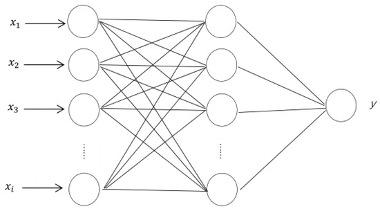
Figure 1. Neural network diagram.

In the above formula, ${\omega }_{ij}(i=1,2,...,m,j=1,2,...,n)$ is the parameter of the model, m is the number of nodes of the input layer, and n is the number of nodes of the hidden layer.

Algorithm steps of the BP neural network:

• Step 1: The sample input and output parameters are normalized to the interval $[0,1]$;
• Step 2: Weight and threshold initialization, assign a random value in $(-1,1)$;
• Step 3: Calculate the state of the hidden layer of the network and the output value of the output layer;
• Step 4: Calculate the error between the output value and the actual value;
• Step 5: Determine whether the sample error is within the acceptable range. If it is satisfied, the training ends. If it is not satisfied, continue to modify the weight and threshold, and go to Step 3 until the error reaches an acceptable range.

The BP neural network parameters (see Table 2) and the network of the learning rate is ${10}^{-4}$.

Table 2. Network parameters.

Country	Parameter	Value
	three-layer structure	6-6-1
CAN	hidden layer function	tansig
	output layer function	purelin
	three-layer structure	4-6-1
FRA	hidden layer function	tansig
	output layer function	purelin
	three-layer structure	7-6-1
ITA	hidden layer function	tansig
	output layer function	purelin
	three-layer structure	5-6-1
JPN	hidden layer function	tansig
	output layer function	purelin
	three-layer structure	7-6-1
GBR	hidden layer function	tansig
	output layer function	purelin
	three-layer structure	6-6-1
USA	hidden layer function	tansig
	output layer function	purelin
	three-layer structure	5-6-1
EUU	hidden layer function	tansig
	output layer function	purelin

In order to measure the performance and predictive capabilities of the BP neural network models, we selected the data from 70% as the training sample, and data from 30% were used as the test sample. In addition, the average absolute deviation (MAD) and the coefficient of determination ($R^2$) were used to evaluate the model, and we used the absolute error to describe the prediction effect of the model. The MAD, $R^2$ and the absolute error are defined as follows:

$$\begin{array}{c}\hfill MAD=\frac{{\displaystyle \sum _{i=1}^n}|y_i-\widehat{y_i}|}{n},\end{array}$$

(7)

and

$$\begin{array}{c}\hfill AR{E}_i=|\frac{y_i-\widehat{y_i}}{y_i}|,i=1,2,...,n,\end{array}$$

(8)

and

$$\begin{array}{c}\hfill R^2=1-\frac{{\displaystyle \sum _{i=1}^n}{(y_i-\widehat{y_i})}^2}{{\displaystyle \sum _{i=1}^n}{(y_i-\overline{y})}^2}.\end{array}$$

(9)

We usually use the BIC to evaluate the quality of a model. The smaller the BIC value, the better the model.

$$\begin{array}{c}\hfill BIC=log(\frac{1}{n}\sum _{i=1}^n{(y_i-{\widehat{y}}_i)}^2)+\frac{plogn}{n}.\end{array}$$

(10)

3. Main Results

3.1. Variable Selection

We used the adaptive lasso method to select variables (see Table 3).

Table 3. Importance of the eight variables on Model (1) for each country.

Country	${\mathit{x}}_1$	${\mathit{x}}_2$	${\mathit{x}}_3$	${\mathit{x}}_4$	${\mathit{x}}_5$	${\mathit{x}}_6$	${\mathit{x}}_7$	${\mathit{x}}_8$
CAN		✓	✓		✓	✓	✓	✓
FRA				✓	✓	✓	✓
DEU	✓			✓	✓		✓
ITA	✓	✓	✓	✓	✓	✓	✓
JPN	✓		✓		✓	✓	✓
GBR		✓	✓	✓	✓	✓	✓	✓
USA			✓	✓	✓	✓	✓	✓
EUU	✓	✓	✓	✓	✓

3.2. The Importance of Input Variables

The result of the training consists of how the BP neural network determines the inputs with the most important influences on the output. Table 4 and Figure 2 show the most influential variables and the smallest influence variables in the training process.

Table 4. The importance of input variables.

Countries	Variables	Importance	The Importance of Standardization
CAN	$x_2$	0.164	88.9%
	$x_3$	0.167	90.7%
	$x_5$	0.164	89.3%
	$x_6$	0.159	86.3%
	$x_7$	0.162	88.0%
	$x_8$	0.184	100.0%
FRA	$x_4$	0.258	93.9%
	$x_5$	0.239	86.9%
	$x_6$	0.275	100.0%
	$x_7$	0.228	83.0%
DEU	$x_1$	0.289	100.0%
	$x_4$	0.220	76.1%
	$x_5$	0.246	85.0%
	$x_7$	0.245	84.8%
ITA	$x_1$	0.122	74.1%
	$x_2$	0.127	77.1%
	$x_3$	0.139	84.0%
	$x_4$	0.165	100.0%
	$x_5$	0.146	88.5%
	$x_6$	0.141	85.7%
	$x_7$	0.159	96.1%
JPN	$x_1$	0.255	100.0%
	$x_3$	0.184	72.1%
	$x_5$	0.204	80.1%
	$x_6$	0.177	69.5%
	$x_7$	0.180	70.5%
GRB	$x_2$	0.131	83.3%
	$x_3$	0.148	94.6%
	$x_4$	0.153	97.3%
	$x_5$	0.129	82.0%
	$x_6$	0.134	85.7%
	$x_7$	0.157	100.0%
	$x_8$	0.148	94.7%
USA	$x_3$	0.176	97.4%
	$x_4$	0.159	87.9%
	$x_5$	0.168	93.2%
	$x_6$	0.167	92.4%
	$x_7$	0.150	83.3%
	$x_8$	0.180	100.0%
EUU	$x_1$	0.178	80.0%
	$x_2$	0.200	90.2%
	$x_3$	0.208	93.5%
	$x_4$	0.222	100.0%
	$x_5$	0.192	86.3%

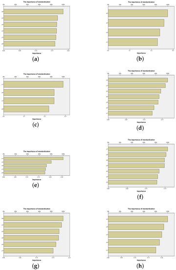
Figure 2. The importance of input variables of the BP neural network model for the G7 countries: (a) Canada (b) France (c) Germany (d) Italy (e) Japan (f) the United Kingdom (g) the United States (h) European Union.

Then, we used the selected variables to establish neural network models of different countries in turn. We calculated the values of MAD, $R^2$, and the BIC index in the training sample set (see Table 5).

Table 5. Different values of neural network.

	MAD	${\mathit{R}}^2$	BIC
CAN	4,979,833,005	0.9997	45.3517
FRA	5,354,234,528	0.9998	45.6559
DEU	14,770,977,340	0.9992	46.9995
ITA	971,799,315,896	0.9999	44.9924
JPN	14,963,447,015	0.9997	57.8385
GBR	895,719,476,802	0.9995	53.0472
USA	27,207,015,544	0.9999	48.9367
EUU	2,269,209,989,327	0.9998	49.7041

3.3. Fitting Result

Now, we give the fitting results of the BP neural network based on R software (the version is 3.6.1) (see Figure 3).

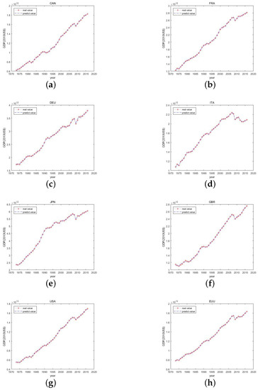
Figure 3. Fitting results for the BP neural network model for the G7 countries: (a) Canada (b) France (c) Germany (d) Italy (e) Japan (f) the United Kingdom (g) the United States (h) European Union.

3.4. Predicted Result

Finally, we present the forecast results of the neural network model for G7 countries with GDP data from 2012–2016, and we indexed values, as shown in Table 6.

Table 6. Neural network model for G7 countries, GDP data from 2012–2016.

	Year	Real Value	Predict Value	${\mathbf{ARE}}_{\mathit{i}}$
	2012	1,693,194,096,275.46	1,700,796,254,959.84	0.004492
	2013	1,735,100,681,636.87	1,728,839,650,854.99	0.003608
CAN	2014	1,779,611,206,826.42	1,773,972,857,272.54	0.003168
	2015	1,796,369,375,909.66	1,804,725,880,265.16	0.004652
	2016	1,822,735,534,879.33	1,819,578,502,324.51	0.001734
	2012	2,706,807,051,174.77	2,705,120,885,014.09	0.000623
	2013	2,722,404,797,996.28	2,723,028,718,241.47	0.000229
FRA	2014	2,748,201,937,555.55	2,757,977,826,977.9	0.003557
	2015	2,777,537,939,261.97	2,779,786,370,549.96	0.000810
	2016	2,810,525,379,194.34	2,804,990,064,602.12	0.001969
	2012	3,559,587,403,262.56	3,502,904,570,253.34	0.015924
	2013	3,577,014,590,829.77	3,608,327,110,971.49	0.008754
DEU	2014	3,646,039,898,346.43	3,634,064,010,446.31	0.003285
	2015	3,709,597,862,509.39	3,707,557,695,995.23	0.000550
	2016	3,781,698,549,834.74	3,768,496,346,567.67	0.003491
	2012	2,077,060,704,620.29	2,076,240,180,028.15	0.000395
	2013	2,041,165,755,679.07	2,045,595,010,254.51	0.002168
ITA	2014	2,043,486,014,884.01	2,043,977,764,656.97	0.000239
	2015	2,063,873,410,309.19	2,064,207,266,781.75	0.000163
	2016	2,083,322,583,449.54	2,078,694,598,826.19	0.002220
	2012	5,778,636,370,123.56	5,788,841,843,578.57	0.001766
	2013	5,894,237,388,118.86	5,842,619,130,629.46	0.008757
JPN	2014	5,914,022,267,462.79	5,943,377,013,580.25	0.004964
	2015	5,986,140,110,537.86	6,005,743,218,991.7	0.003275
	2016	6,047,894,004,051.61	6,028,452,852,492.38	0.003215
	2012	2,513,321,589,693.39	2,509,553,645,802.85	0.001499
	2013	2,564,904,713,179.98	2,574,393,456,751.26	0.003701
GBR	2014	2,643,243,341,332.76	2,646,191,494,885.59	0.001117
	2015	2,705,252,231,411.39	2,717,092,799,299.32	0.004378
	2016	2,753,793,133,582.5	2,733,135,616,113.89	0.007500
	2012	15,542,161,722,300	15,584,345,914,523.5	0.002714
	2013	15,802,855,301,300	15,863,586,662,748.6	0.003843
USA	2014	16,208,861,247,400	16,251,038,963,537.9	0.002602
	2015	16,672,691,917,800	16,674,989,794,495	0.000138
	2016	16,920,327,941,800	1,682,106,154,6143.1	0.005867
	2012	17,206,500,000,000	17,097,457,864,107.1	0.006337
	2013	17,251,100,000,000	17,252,390,426,035.3	0.000075
EUU	2014	17,551,100,000,000	17,637,790,796,812.8	0.004939
	2015	17,957,000,000,000	17,978,401,657,980.2	0.001192
	2016	18,305,200,000,000	18,277,752,838,514.5	0.001499

All the figures and tables are the results of our research.

4. Conclusions

Differently to the approach in [8], the BP neural network in the economic model was used to study GDP growth in a group of seven countries. By comparing the fitting effect, one can find that the BP neural network model is more efficient than the fractional order model in [8]. In addition, the model also shows the variables that have the greatest impact and the smallest impact on the GDP of different countries. Meanwhile, we found that the input layer variables of the neural network model had different impacts on the output layer. To further illustrate the forecasting effect of the BP neural network model, we presented the GDP forecast for G7 countries from 2012-2016 and compared it with the real value. It was found that the BP neural network model not only had an advantage in fitting the G7 countries’ GDP growth, but also predicted it better. Finally, because the BP neural network had problems involving slower convergence and local extremum, we intend to extend our study by applying a hybrid genetic algorithm to optimize the structure and parameter of BP (back propagation) neural networks based on the gradient descent of multi-encoding.

References

- Sadeghi, B. A BP-neural network predictor model for plastic injection molding process. J. Inequal. J. Mater. Process Technol. 2000, 103, 411–416. [Google Scholar] [CrossRef]
- Xiao, Z.; Ye, S.; Zhong, B.; Sun, C. BP neural network with rough set for short term load forecasting. Appl. Artif. Intell. Rev. 2009, 36, 273–279. [Google Scholar] [CrossRef]
- Yu, S.; Zhu, K.; Diao, F. A dynamic all parameters adaptive BP neural networks model and its application on oil reservoir prediction. Appl. Math. Comput. 2008, 195, 66–75. [Google Scholar] [CrossRef]
- Guo, Z.; Wu, J.; Lu, H.; Wang, J. A case study on a hybrid wind speed forecasting method using BP neural network. Knowl.-Based Syst. 2011, 24, 1048–1056. [Google Scholar] [CrossRef]
- Feng, L.; Zhang, J. Application of artificial neural networks in tendency forecasting of economic growth. Am. Econ. J.-Econ. Polic. 2014, 40, 76–80. [Google Scholar] [CrossRef]
- Wang, H.; Leng, C. A note on adaptive group lasso. Appl. Comput. Stat. Data Anal. 2008, 52, 5277–5286. [Google Scholar] [CrossRef]
- Ren, Y.; Zhang, X. Model Selection for Vector Autoregressive Processes via Adaptive Lasso. Commun. Stat.-Theory Methods 2013, 42, 2423–2436. [Google Scholar] [CrossRef]
- Tejado, I.; Pérez, E.; Valxexrio, D. Fractional calculus in economic growth modelling of the group of seven. Fract. Calc. Appl. Anal. 2019, 22, 139–157. [Google Scholar] [CrossRef]
- Ming, H.; Wang, J.; Fečkan, M. The application of fractional calculus in Chinese economic growth models. Mathematics 2019, 7, 665. [Google Scholar] [CrossRef]
- Gerardo-Giorda, L.; Germano, G.; Scalas, E. Large-scale simulations of synthetic markets. Commun. Appl. Ind. Math. 2014, 6, 535–842. [Google Scholar]
- Tarasov, V.E.; Tarasova, V.V. Dynamic Keynesian model of economic growth with memory and lag. Mathematics 2019, 7, 178. [Google Scholar] [CrossRef]
- Tarasova, V.V.; Tarasov, V.E. Elasticity for economic processes with memory: Fractional differential calculus approach. Fract. Differ. Calc. 2016, 6, 219–232. [Google Scholar] [CrossRef]
- Luo, D.; Wang, J.; Fečkan, M. Applying Fractional calculus to analyze economic growth modelling. J. Appl. Math. Stat. Inform. 2018, 14, 25–36. [Google Scholar] [CrossRef]
- Tarasov, V.E.; Tarasova, V.V. Macroeconomic models with long dynamic memory: Fractional calculus approach. Appl. Math. Comput. 2018, 338, 466–486. [Google Scholar] [CrossRef]
- Zou, H. The adaptive lasso and its oracle properties. J. Am. Stat. Assoc. 2006, 101, 1418–1492. [Google Scholar] [CrossRef]
- Fulger, D.; Scalas, E.; Germano, G. Monte Carlo simulation of uncoupled continuous-time random walksyielding a stochastic solution of the space-time fractional diffusion equation. Phys. Rev. E 2008, 77, 021122. [Google Scholar] [CrossRef]
- Fan, J.; Li, R. Variable selection via nonconcave penalized likelihood and its oracle properties. J. Am. Stat. Assoc. 2011, 96, 1348–1360. [Google Scholar] [CrossRef]
- Shojaie, A.; Michailidis, G. Penalized likelihood methods for estimation of sparse high-dimensional directed acyclic graphs. Biometrika 2010, 97, 519–538. [Google Scholar] [CrossRef]
© 2020 by the authors. Licensee MDPI, Basel, Switzerland. This article is an open access article distributed under the terms and conditions of the Creative Commons Attribution (CC BY) license (http://creativecommons.org/licenses/by/4.0/).