Stanley Depth of Edge Ideals of Some Wheel-Related Graphs

Abstract

Stanley depth is a geometric invariant of the module and is related to an algebraic invariant called depth of the module. We compute Stanley depth of the quotient of edge ideals associated with some familiar families of wheel-related graphs. In particular, we establish general closed formulas for Stanley depth of quotient of edge ideals associated with the $mth$-power of a wheel graph, for $m\ge 3$, gear graphs and anti-web gear graphs.

1. Introduction

Richard P. Stanley is famous for his contribution to combinatorial aspects of algebra and geometry. Simplicial complexes are critical objects in combinatorics; two of the most important such complexes are partitionable and Cohen–Macauly complexes. Stanley introduced the famous conjecture relating these two complexes and hence, introduced the notion of Stanley depth in 1982 in [1]. Stanley Depth is a geometric invariant of module. The Stanley conjecture is interesting in the sense that it compares a combinatorial invariant with a homological invariant of module. Stanley depth gained attention of algebraists in 2006 when J. Herzog and D. Popescu studied this conjecture. Afterwards, a number of articles have been published in which this conjecture has been discussed for different cases. Let $S=K[x_1,x_2,...,x_n]$ be a polynomial ring in n variables over a field K and M be finitely generated ${\mathbb{Z}}^n$-graded S-module. For a homogeneous element $q\in M$ and a subset $Z\subseteq \{x_1,x_2,...,x_n\}$, $qK\left[Z\right]$ denotes the K-subspace of M generated by all homogeneous elements of the form $qv$, where v is a monomial in $K\left[Z\right]$. The space $qK\left[Z\right]$ is ${\mathbb{Z}}^n$-graded K-subspace and is called $Stanleyspace$ of dimension $\left|Z\right|$ if it is a free $K\left[Z\right]$-module, where $\left|Z\right|$ denotes the cardinality of Z. A decomposition of M as a finite direct sum of ${\mathbb{Z}}^n$-graded K-vector spaces is called Stanley decomposition.

$$\mathcal{D}:M=\underset{j=1}{\overset{s}{⨁}}{q}_{j}K\left[Z_j\right]$$

where each $q_{j}K\left[Z_j\right]$ is a Stanley space of M. The number

$$\mathrm{sdepth}\left(\mathcal{D}\right)=\min \left\{\right|Z_j|:j=1,2,3,...,s\}$$

is called Stanley depth of decomposition $\mathcal{D}$ and the quantity

$$\mathrm{sdepth}\left(M\right)=\max \left\{\mathrm{sdepth}\right(\mathcal{D}\left)\right|\mathcal{D}isaStanleydecompositionofM\}$$

is called Stanley depth of M.

Richard P. Stanley [1] in his article “Linear Diophantine equation and local cohomology” stated this conjecture, in a generalized way, as follows:

Let R be a finitely generated ${\mathbb{N}}^n$-graded K-algebra ($R_0=K$) and let M be a finitely generated ${\mathbb{Z}}^n$-graded R-module. Then there exist finitely many subalgebras $S_1,...,S_t$ of R, each generated by algebraically independent ${\mathbb{N}}^n$-homogeneous elements of R, and there exist ${\mathbb{Z}}^n$-homogeneous elements ${\eta }_1,...,{\eta }_t$ of M, such that

$$M=\underset{i=1}{\overset{t}{⨁}}{\eta }_i{S}_i$$

where $dim\left(S_i\right)\ge depth\left(M\right)$ for all i, and where ${\eta }_i{S}_i$ is a free $S_i$-module and where ${⨁}_{i=1}^t$ is finite direct sum of modules ${\eta }_i{S}_i$.“ The direct sum of modules is a new module defined as ${⨁}_{i\in I}{M}_i=\{(m_i\in M_i)i\in I\mid m_i=0$ for but finitely many $i\}$.

In [2], the authors found an upper bound for the Stanley depth of $S/Q\cap Q^{\prime }$, where S is polynomial ring and $Q,Q^{\prime }$ are monomial primary ideals and also showed that this conjecture holds for $Q_1\cap Q_2$ and $S/Q_1\cap Q_2\cap Q_3$, where $Q_1,Q_2,Q_3$ are monomial irreducible ideals. In [3], authors found upper bound for Stanley depth of edge ideals of k-partite complete graph and s-uniform complete bipartite hyper = graph. In [4], authors found upper bound for the Stanley depth of edge ideals of complete graph and complete bipartite graph when some variables are added as generators. In [5], the authors gave the lower and upper bound for the cyclic module associated with the complete k-partite hyper-graph. Duval et al. disproved this conjecture in [6]. A method to compute Stanley depth for the module M, where M is of the form $M=I/J$, where $J\subset I\subset S$ are monomial ideals, was given by Herzog, Vladoiu and Zheng in [7]. Rinaldo developed this method into an algorithm in [8] which is implemented in CoCoA [9]. In [10], Rauf proved some important basic results regrading depth and Stanley depth of multi-graded module. Stanley depth of the edge ideal associated with some graphs have been subject matter of recent results. In [11], Cimpoeas computed Stanley depth of the edge ideal of line and cycles. Iqbal et al. computed Depth and sdepth of edge ideals of square paths and square cycles in [12]. Stanley depth of edge ideals of general powers of path ideals is computed in [13]. In [14], Cimpoeas proved several inequalities regarding computation of Stanley depth. Let $I\left(P_n\right)$ denote the edge ideal associated with path on n vertices. Then bounds and values for Stanley depth and depth for module $S/I\left(P_n\right)$ are given in [11,12,13]. Stanley depth of the quotient of edge ideal associated with wheel graph and square wheel graph is computed in [15]. In paper [16], Biro et al. discussed interval partition associated with partially ordered set which is required to find Stanley depth, and also how this interval partition is used to find out Stanley depth. Cimpoeas, in [17] discussed Stanley depth of modules having small number of generators. For the friendly introduction to commutative algebra, we refer readers to [18].

We set $S_m=K[x_1,x_2,x_3,...,x_m]$, $\mathrm{supp}\left(u\right)=\{i:x_i|u\}$ and $\mathrm{supp}\left(J\right)=\{i:x_i|v\mathrm{for}\mathrm{some}v\in G\left(J\right)\}$ where $G\left(J\right)$ denotes the unique minimal set of monomial generators of the monomial ideal J for the rest of this article.

2. Example

We explain Stanley decomposition and Stanley depth with the help of an example. We present some graphical representations which are used to construct a particular Stanley decomposition which are explained briefly in [7].

Let $S=K[x_1,x_2]$ and $I=(x_1^3,x_1^2{x}_2,x_2^2)$ be a monomial ideal. Since we know that one module can have many Stanley decompositions, see for example Figure 1.

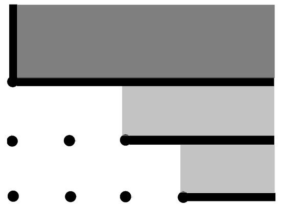
Figure 1. Decomposition $D_1$.

In the Figure 1, decomposition $D_1$ of I is shown graphically given as,

$$D_1:I=x_1^{3}K\left[x_1\right]\oplus x_1^2{x}_{2}K\left[x_1\right]\oplus x_2^{2}K[x_1,x_2].$$

Now we give another decomposition to explain further. In the Figure 2, decomposition $D_2$ of I is shown graphically as

$$D_2:I=x_2^{2}K\left[x_2\right]\oplus x_1{x}_2^{2}K\left[x_2\right]\oplus x_1^2{x}_{2}K\left[x_2\right]\oplus x_1^{3}K[x_1,x_2].$$

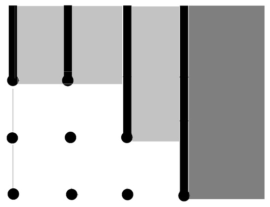
Figure 2. Decomposition $D_2$.

Clearly the $sdepth\left(I\right)=1$ because in decomposition $D_2$ of I, Stanley spaces have dimensions $1,1,1$ and 2 respectively. So the smallest in all these dimensions is 1 and called Stanley depth of I. For further and detailed reading, we refer to [7].

The Stanley decomposition of $S/I$ is given as

$$D:S/I=K\oplus x_{1}K\oplus x_1^{2}K\oplus x_{2}K\oplus x_1{x}_{2}K,$$

hence, we see that $sdepth(S/I)=0$.

Definition 1.

Edge ideal: Let $G=\left(V\right(G),E(G\left)\right)$ be a graph with edge set $E\left(G\right)$ and vertex set $V\left(G\right)=\{1,2,...,n\}$ then the edge ideal associated with G is the square free monomial ideal of S, defined as

$$I\left(G\right)=(x_l{x}_k:\{l,k\}\in E\left(G\right)).$$

Definition 2.

$mth$-power of wheel graph: Let $n\ge 5$ and ${\mathcal{W}}_n^m$ be a $mth$-power of wheel on n vertices, then the edge ideal of $mth$-power of Wheel is

$$\begin{array}{c}\hfill \left(I\left(W_n^m\right)\right)=(x_1{x}_n,x_2{x}_n,x_3{x}_n,...,x_{n-1}{x}_n,x_1{x}_2,x_2{x}_3,...,x_{n-1}{x}_1,x_1{x}_3,x_2{x}_4,...,x_{n-1}{x}_2,\\ \hfill x_1{x}_4,x_2{x}_5,...,x_{n-1}{x}_3,...,x_1{x}_m,x_2{x}_{m+1},...,x_{n-1}{x}_{m-1},x_1{x}_{m+1},x_2{x}_{m+2},...,x_{n-1}{x}_m).\end{array}$$

An example of graph of $I\left(W_7^2\right)$ is given in Figure 3.

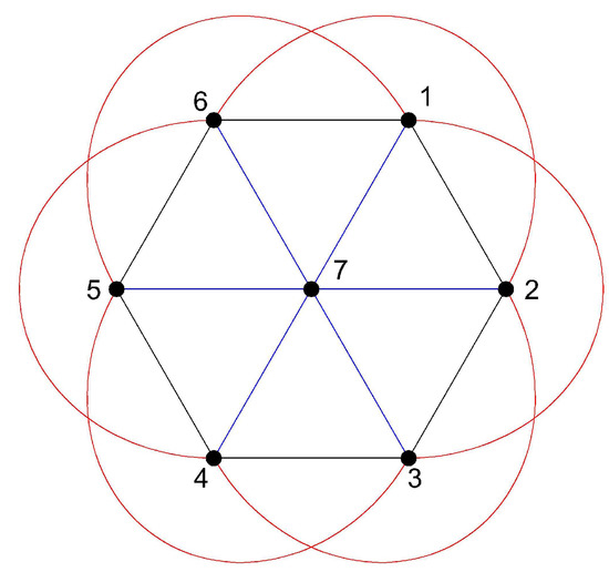
Figure 3. Graph of $I\left(W_7^2\right)$.

Definition 3.

Gear graph: The gear graph $G_n$, where $n\in \{5,7,9,...,\}$ consists of cycle of $n-1$ vertices and the vertex n joins with vertices $1,3,5,7,...,n-1$.

The edge ideal $I\left(G_n\right)$ of the gear graph is defined as

$$\begin{array}{c}\hfill I\left(G_n\right)=(x_1{x}_2,x_2{x}_3,x_3{x}_4,...,x_{n-2}{x}_{n-1},x_{n-1}{x}_1,x_1{x}_n,x_3{x}_n,x_5{x}_n,...,x_{n-2}{x}_n).\end{array}$$

The graph of $I\left(G_{11}\right)$ is given in Figure 4.

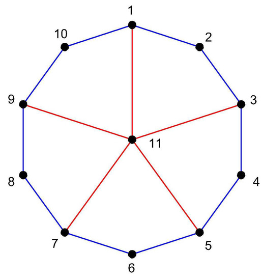
Figure 4. Graph of $I\left(G_{11}\right)$.

Definition 4.

Anti-web gear graph: The anti-web gear graph denoted by $AW{G}_n$, where $n\in \{9,11,13...,\}$ consists of cycle of $n-1$ vertices and also the edges joining vertices having distance two between them on this cycle. And the vertex n joins with vertices $1,3,5,7,...,n-2$. The order of this graph is n.

The edge ideal $I\left(AW{G}_n\right)$ of the Gear graph is defined as

$$\begin{array}{c}\hfill I\left(AW{G}_n\right)=(x_1{x}_2,x_2{x}_3,x_3{x}_4,...,x_{n-2}{x}_{n-1},x_{n-1}{x}_1,x_1{x}_3,x_2{x}_4,x_3{x}_5,...,x_{n-2}{x}_1,x_{n-1}{x}_2,\\ \hfill x_1{x}_n,x_3{x}_n,x_5{x}_n,...,x_{n-2}{x}_n).\end{array}$$

The graph of $I\left(AW{G}_9\right)$ is given in Figure 5.

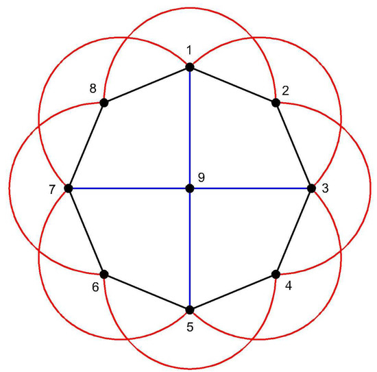
Figure 5. Graph of $I\left(AW{G}_9\right)$.

Following important Lemmas will play significant role in our computation. A short exact sequence of Modules is $0\to M_1\to M_2\to M_3\to 0$ where arrows are maps such that the third map is surjective, second map is injective along with the property that kernel of the third map is same as that of image of second map.

Lemma 1

([10]). Let $0\to U\to V\to W\to 0$ be a short exact sequence of ${\mathbb{Z}}^n$-graded S-modules. Then

$$\mathrm{sdepth}\left(V\right)\ge \min \left\{\mathrm{sdepth}\right(U),\mathrm{sdepth}(W\left)\right\}.$$

Lemma 2

([12]). Let $J\subset S$ be a square free monomial ideal such that $supp\left(J\right)=\left[n\right]$, let $w=x_{j_1}{x}_{j_2}{x}_{j_3}...x_{j_t}\in S/J$, such that, $x_{i}w\in I$, for all $i\in \left[n\right]\setminus supp\left(w\right)$. Then $\mathrm{sdepth}(S/J)\le t$.

For example is $S=K[x_1,x_2,x_3,...,x_n]$ is a polynomial ring in n variables over a field K and $I\left(P_n^3\right)$ is a cube of path whose ideal is given as

$$I\left(P_n^3\right)=(x_1{x}_2,x_2{x}_3,...,x_{n-1}{x}_n,x_1{x}_3,x_2{x}_4,...,x_{n-2}{x}_n,x_1{x}_4,x_2{x}_5,...,x_{n-3}{x}_n).$$

Then Stanley decomposition for the following cases by [7] is given as

$$\begin{array}{c}\hfill Ifn=3.Then,S/I\left(P_3^3\right)=K\left[x_1\right]\oplus x_{2}K\left[x_2\right]\oplus x_{3}K\left[x_3\right].\\ \hfill Ifn=4.Then,S/I\left(P_4^3\right)=K\left[x_1\right]\oplus x_{2}K\left[x_2\right]\oplus x_{3}K\left[x_3\right]\oplus x_{4}K\left[x_4\right].\\ \hfill Ifn=5.Then,S/I\left(P_5^3\right)=K[x_1,x_5]\oplus x_{2}K\left[x_2\right]\oplus x_{3}K\left[x_3\right]\oplus x_{4}K\left[x_4\right].\end{array}$$

In this paper we are interested in computing Stanley depth of the quotient of $mth$-power of Wheel graph, gear graph and anti-web gear graph.

3. Main Result

In this section we are going to compute our main results.

Theorem 1.

Let $n\ge 6$, and $I\left({\mathcal{W}}_n^m\right)$ be an ideal of wheel graph on n vertices, then sdepth $(S/I\left({\mathcal{W}}_n^m\right))=1$.

Proof. 

The ideal of $mth$-power of Wheel graph is given as

$$\begin{array}{c}\hfill \left(I\left({\mathcal{W}}_n^m\right)\right)=(x_1{x}_n,x_2{x}_n,x_3{x}_n,...,x_{n-1}{x}_n,x_1{x}_2,x_2{x}_3,...,x_{n-1}{x}_1,x_1{x}_3,x_2{x}_4,...,x_{n-1}{x}_2,\\ \hfill x_1{x}_4,x_2{x}_5,...,x_{n-1}{x}_3,...,x_1{x}_m,x_2{x}_{m+1},...,x_{n-1}{x}_{m-1},x_1{x}_{m+1},x_2{x}_{m+2},...,x_{n-1}{x}_m).\end{array}$$

Now consider a short exact sequence by taking functions $\psi :(I\left({\mathcal{W}}_n^m\right):x_n)\to \left(I\left({\mathcal{W}}_n^m\right)\right)$ such that $\psi \left(r\right)=x_{n}r$ is a multiplication by $x_n$ and $\phi :\left(I\left({\mathcal{W}}_n^m\right)\right)\to (I\left({\mathcal{W}}_n^m\right),x_n)$ such that $\phi \left(r\right)=r$. Throughout this paper we use similar kind of functions to make our sequence of modules short exact.

$$0\to S/(I\left({\mathcal{W}}_n^m\right):x_n)\to S/\left(I\left({\mathcal{W}}_n^m\right)\right)\to S/(I\left({\mathcal{W}}_n^m\right),x_n)\to 0.$$

by Lemma 1

$$\mathrm{sdepth}(S/\left(I\left({\mathcal{W}}_n^m\right)\right))\ge \min \left\{\mathrm{sdepth}(S/\left({\mathcal{W}}_n^m\right):x_n)\right),\mathrm{sdepth}(S/(I\left({\mathcal{W}}_n^m\right),x_n))\}.$$

Here

$$(I\left({\mathcal{W}}_n^m\right):x_n)=(x_1,x_2,x_3,x_4,...,x_{n-1}).So(S/(I\left(W_n^m\right):x_n))\cong K\left[x_n\right].$$

Hence $\mathrm{sdepth}(S/(I\left({\mathcal{W}}_n^m\right):x_n))=1$.

And

$$\begin{array}{c}\hfill (I\left({\mathcal{W}}_n^m\right),x_n)=(x_1{x}_2,x_2{x}_3,...,x_{n-1}{x}_1,x_1{x}_3,x_2{x}_4,...,x_{n-1}{x}_2,\\ \hfill x_1{x}_4,x_2{x}_5,...,x_{n-1}{x}_3,...,x_1{x}_m,x_2{x}_{m+1},...,x_{n-1}{x}_{m-1},x_1{x}_{m+1},x_2{x}_{m+2},...,x_{n-1}{x}_m,x_n).\end{array}$$

where $S/(I\left({\mathcal{W}}_n^m\right),x_n)\cong S_{n-1}/I\left(C_{n-1}^m\right)$ and $\mathrm{sdepth}(S/(I\left({\mathcal{W}}_n^m\right),x_n))=\mathrm{sdepth}(S_{n-1}/I\left(C_{n-1}^m\right))\ge ⌈\frac{(n-1)-m}{2m+1}⌉$ by [19].

Here $⌈\frac{(n-1)-m}{2m+1}⌉\ge 1,$ because if $n-1\le m$ then we have two cases. If $n-1=2k$, where $k\ge 3$ then we can check that $I\left(C_{2k}^m\right)=I\left(C_{2k}^k\right)$. And if $n-1=2k+1$, then can see that $I\left(C_{2k+1}^m\right)=I\left(C_{2k+1}^k\right)$, so we get the desired result for both these cases. So $\mathrm{sdepth}(S/(I\left({\mathcal{W}}_n^m\right):x_n))=1\le \mathrm{sdepth}(S/(I\left({\mathcal{W}}_n^m\right),x_n))$. This implies that $\mathrm{sdepth}(S/\left(I\left({\mathcal{W}}_n^m\right)\right))\ge \mathrm{sdepth}(S/(I\left({\mathcal{W}}_n^m\right):x_n))=1.$ We get the other inequality by Proposition 2.7 in [14]. Hence $\mathrm{sdepth}(S/\left(I\left({\mathcal{W}}_n^m\right)\right))=\mathrm{sdepth}(S/(I\left({\mathcal{W}}_n^m\right):x_n))=1$. □

Theorem 2.

Let $n\ge 5$ and is an odd number, then sdepth $(S/I\left(G_n\right))\ge ⌈\frac{n-2}{3}⌉$.

Proof. 

We have

$$\begin{array}{c}\hfill I\left(G_n\right)=(x_1{x}_2,x_2{x}_3,x_3{x}_4,...,x_{n-2}{x}_{n-1},x_{n-1}{x}_1,x_1{x}_n,x_3{x}_n,x_5{x}_n,...,x_{n-2}{x}_n).\end{array}$$

Consider the following short exact sequence

$$\begin{array}{c}\hfill 0\to S/(I\left(G_n\right):x_n)\to S/I\left(G_n\right)\to S/(I\left(G_n\right),x_n)\to 0.\end{array}$$

By Lemma 1

$$\mathrm{sdepth}(S/\left(I\left(G_n\right)\right)\ge \min \{\mathrm{sdepth}(S/(I\left(G_n\right):x_n)),\mathrm{sdepth}(S/(I\left(G_n\right),x_n))\}.$$

Here

$$\begin{array}{c}\hfill (I\left(G_n\right),x_n)=(x_1{x}_2,x_2{x}_3,x_3{x}_4,...,x_{n-2}{x}_{n-1},x_{n-1}{x}_1,x_n).\end{array}$$

So $S/(I\left(G_n\right),x_n)\cong S_{n-1}/I\left(C_{n-1}\right).$ Hence by Theorem 1.9 of [11] sdepth $(S/(I\left(G_n\right),x_n))\ge ⌈\frac{n-2}{3}⌉.$

And

$$\begin{array}{c}\hfill (I\left(G_n\right):x_n)=(x_1,x_3,x_5,...,x_{n-2}).\end{array}$$

So we have $S/(I\left(G_n\right):x_n)\cong K[x_2,x_4,x_6,...,x_{n-1},x_n].$

Hence sdepth $(S/(I\left(G_n\right):x_n))\ge ⌈\frac{n}{2}⌉$.

So we get sdepth $(S/\left(I\left(G_n\right)\right)\ge$ sdepth $(S/(I\left(G_n\right),x_n)),$ sdepth $(S/\left(I\left(G_n\right)\right)\ge ⌈\frac{n-2}{3}⌉$. □

Theorem 3.

Let $n\ge 5$, then sdepth $(S/\left(I\left(G_n\right)\right))=⌈\frac{n}{3}⌉$, for $n\equiv 0$ (mod 3).

The sdepth $(S/\left(I\left(G_n\right)\right))=⌈\frac{n}{3}⌉$ − 1, for $n\equiv 1$ (mod 3).

And when $n\equiv 2$ (mod 3), then $⌈\frac{n-2}{3}⌉\le$ sdepth $(S/\left(I\left(G_n\right)\right))\le ⌈\frac{n}{3}⌉$.

Proof. 

We prove this result by the following three cases.

Case 1: When $n=3q$, where $q\in \{3,5,7,...\}$. Then by Theorem 2 we can see sdepth $(S/\left(I\left(G_n\right)\right)\ge ⌈\frac{n}{3}⌉.$

Now we have to show the other inequality.

Since $w=x_1{x}_4{x}_7...x_{\left(3\right(q-2)+1)}{x}_{3(q-1)+1}\in S/\left(I\left(G_n\right)\right)$, but $x_{i}w\in I\left(G_n\right)$, for all $i\in \left[n\right]\setminus \mathrm{supp}\left(w\right)$, therefore by Lemma 2, $\mathrm{sdepth}(S/\left(I\left(G_n\right)\right))\le q=\lceil \frac{n}{3}\rceil$.

Case 2: When $n=3q+1$, where $q\in \{2,4,6,...\}$. Then by Theorem 2 we can see sdepth $(S/\left(I\left(G_n\right)\right)\ge ⌈\frac{(3q+1)-2}{3}⌉=q=$$⌈\frac{n}{3}⌉-1.$

Now to prove the other inequality.

Since $w=x_1{x}_4{x}_7...x_{\left(3\right(q-2)+1)}{x}_{3(q-1)+1}\in S/\left(I\left(G_n\right)\right)$, but $x_{i}w\in I\left(G_n\right)$, for all $i\in \left[n\right]\setminus \mathrm{supp}\left(w\right)$, therefore by Lemma 2, $\mathrm{sdepth}(S/\left(I\left(G_n\right)\right))\le q=\lceil \frac{n}{3}\rceil -1$.

Case 3: When $n=3q+2$, where $q\in \{1,3,5,7,...\}$. Then by Theorem 2 we can see sdepth $(S/\left(I\left(G_n\right)\right)\ge ⌈\frac{n-2}{3}⌉$.

To show the other inequality.

Since $w=x_1{x}_4{x}_7...x_{\left(3\right(q-1)+1)}{x}_{3q}\in S/\left(I\left(G_n\right)\right)$, but $x_{i}w\in I\left(G_n\right)$, for all $i\in \left[n\right]\setminus \mathrm{supp}\left(w\right)$, therefore by Lemma 2, $\mathrm{sdepth}(S/\left(I\left(G_n\right)\right))\le q+1=⌈\frac{n}{3}⌉$. □

Theorem 4.

Let $n\ge 9$ and is an odd number, then sdepth $(S/I\left(AW{G}_n\right))\ge ⌈\frac{n-3}{5}⌉$.

Proof. 

We have

$$\begin{array}{c}\hfill I\left(AW{G}_n\right)=(x_1{x}_2,x_2{x}_3,x_3{x}_4,...,x_{n-2}{x}_{n-1},x_{n-1}{x}_1,x_1{x}_3,x_2{x}_4,...,x_{n-2}{x}_1,x_{n-1}{x}_2,\\ \hfill x_1{x}_n,x_3{x}_n,...,x_{n-2}{x}_n).\end{array}$$

Consider the following short exact sequence

$$\begin{array}{c}\hfill 0\to S/(I\left(AW{G}_n\right):x_n)\to S/I\left(AW{G}_n\right)\to S/(I\left(AW{G}_n\right),x_n)\to 0.\end{array}$$

Here

$$\begin{array}{c}\hfill (I\left(AW{G}_n\right):x_n)=(x_1,x_3,x_5,...,x_{n-2}).\end{array}$$

So $(S/(I\left(AW{G}_n\right):x_n))\cong K[x_2,x_4,x_6,...,x_{n-1},x_n].$

We get sdepth $(S/(I\left(AW{G}_n\right):x_n))\ge ⌈\frac{n}{2}⌉$, and

$$\begin{array}{c}\hfill (I\left(AW{G}_n\right),x_n)=(x_1{x}_2,x_2{x}_3,x_3{x}_4,...,x_{n-2}{x}_{n-1},x_{n-1}{x}_1,x_1{x}_3,\\ \hfill x_2{x}_4,...,x_{n-2}{x}_1,x_{n-1}{x}_2,x_n).\end{array}$$

So we have $(S/(I\left(AW{G}_n\right),x_n))\cong S_{n-1}/I\left(C_{n-1}^2\right)$, where $I(C_{n-1}^2$ is a square cycle on $n-1$ vertices. By using [8,12] we get sdepth $(S/(I\left(AW{G}_n\right),x_n))\ge ⌈\frac{n-3}{5}⌉$. By applying Lemma 1 we have

$$\mathrm{sdepth}(S/\left(I\left(AW{G}_n\right)\right)\ge \min \{\mathrm{sdepth}(S/(I\left(AW{G}_n\right):x_n)),\mathrm{sdepth}(S/(I\left(AW{G}_n\right),x_n))\}.$$

So we get sdepth $(S/\left(I\left(AW{G}_n\right)\right))\ge$ sdepth $(S/(I\left(AW{G}_n\right),x_n))$.

Hence sdepth $(S/\left(I\left(AW{G}_n\right)\right))\ge ⌈\frac{n-3}{5}⌉$. □

Theorem 5.

Let $n\ge 9$ and is an odd number, then sdepth $(S/\left(I\left(AW{G}_n\right)\right))=⌈\frac{n}{5}⌉$, when $n\equiv 0,4$ (mod 5).

For $n\equiv 1$ (mod 5), the sdepth $(S/\left(I\left(AW{G}_n\right)\right))=⌈\frac{n}{5}⌉-1.$

And when $n\equiv 2,3$ (mod 5), then $⌈\frac{n}{5}⌉-1\le$ sdepth $(S/\left(I\left(AW{G}_n\right)\right))\le ⌈\frac{n}{5}⌉.$

Proof. 

We will prove this result by following cases.

Case 1: When $n=5q$, where $q\in \{3,5,7,...\}$. Then by Theorem 4 we can see sdepth $(S/\left(I\left(AW{G}_n\right)\right)\ge ⌈\frac{n}{5}⌉$.

Now we have to show the other inequality.

Since $w=x_1{x}_6{x}_{11}...x_{\left(5\right(q-1)+1)}\in S/\left(I\left(AW{G}_n\right)\right)$, but $x_{i}w\in I\left(AW{G}_n\right)$, for all $i\in \left[n\right]\setminus \mathrm{supp}\left(w\right)$, therefore by Lemma 2, $\mathrm{sdepth}(S/\left(I\left(AW{G}_n\right)\right))\le q=\lceil \frac{n}{5}\rceil$.

Case 2: When $n=5q+1$, where $q\in \{2,4,6,...\}$. Then by Theorem 4 we can see sdepth $(S/\left(I\left(AW{G}_n\right)\right)\ge ⌈\frac{n}{5}⌉-1$.

Now to show the other inequality.

Since $w=x_1{x}_6{x}_{11}...x_{\left(5\right(q-1)+1)}\in S/\left(I\left(AW{G}_n\right)\right)$, but $x_{i}w\in I\left(AW{G}_n\right)$, for all $i\in \left[n\right]\setminus \mathrm{supp}\left(w\right)$, therefore by Lemma 2, $\mathrm{sdepth}(S/\left(I\left(AW{G}_n\right)\right))\le q=\lceil \frac{n}{5}\rceil -1$.

Case 3: When $n=5q+2$, where $q\in \{3,5,7,...\}$. Then by Theorem 4 we can see sdepth $(S/\left(I\left(AW{G}_n\right)\right)\ge ⌈\frac{n}{5}⌉-1$.

Now we have to show the other inequality.

Since $w=x_1{x}_6{x}_{11}...x_{\left(5\right(q-1)+1)}{x}_{\left(5\right(q)-1)}\in S/\left(I\left(AW{G}_n\right)\right)$, but $x_{i}w\in I\left(AW{G}_n\right)$, for all $i\in \left[n\right]\setminus \mathrm{supp}\left(w\right)$, therefore by Lemma 2, $\mathrm{sdepth}(S/\left(I\left(AW{G}_n\right)\right))\le q+1=\lceil \frac{n}{5}\rceil$.

Case 4: When $n=5q+3$, where $q\in \{2,4,6,...\}$. Then by Theorem 4 we can see sdepth $(S/\left(I\left(AW{G}_n\right)\right)\ge ⌈\frac{n}{5}⌉-1$.

Now we have to show the other inequality. Since $w=x_1{x}_6{x}_{11}...x_{\left(5\right(q-1)+1)}{x}_{5q}\in S/\left(I\left(AW{G}_n\right)\right)$, but $x_{i}w\in I\left(AW{G}_n\right)$, for all $i\in \left[n\right]\setminus \mathrm{supp}\left(w\right)$, therefore by Lemma 2, $\mathrm{sdepth}(S/\left(I\left(AW{G}_n\right)\right))\le q+1=\lceil \frac{n}{5}\rceil$.

Case 5: When $n=5q+4$, where $q\in \{1,3,5,...\}$. Then by Theorem 4 we can see sdepth $(S/\left(I\left(AW{G}_n\right)\right)\ge ⌈\frac{n}{5}⌉$.

Now we have to show the other inequality.

Since $w=x_1{x}_6{x}_{11}...x_{\left(5\right(q-1)+1)}{x}_{\left(5q\right)+1}\in S/\left(I\left(AW{G}_n\right)\right)$, but $x_{i}w\in I\left(AW{G}_n\right)$, for all $i\in \left[n\right]\setminus \mathrm{supp}\left(w\right)$, therefore by Lemma 2, $\mathrm{sdepth}(S/\left(I\left(AW{G}_n\right)\right))\le q+1=\lceil \frac{n}{5}\rceil$. □

4. Examples

Now we give some examples of our main results.

Example 1.

Let $I\left({\mathcal{W}}_7^2\right)$ be an edge ideal of square wheel graph as shown in Figure 3, then we have to show that sdepth $(S/I\left({\mathcal{W}}_7^2\right))=1$. The edge ideal of the square wheel graph is given as

$$\begin{array}{c}\hfill I\left({\mathcal{W}}_7^2\right)=(x_1{x}_7,x_2{x}_7,x_3{x}_7,...,x_6{x}_7,x_1{x}_2,x_2{x}_3,x_3{x}_4,...,x_6{x}_1,\\ \hfill x_1{x}_3,x_2{x}_4,x_3{x}_5,...,x_6{x}_2).\end{array}$$

Now consider a short exact sequence

$$0\to S/(I\left({\mathcal{W}}_7^2\right):x_7)\to S/\left(I\left({\mathcal{W}}_7^2\right)\right)\to S/(I\left({\mathcal{W}}_7^2\right),x_7)\to 0$$

by Lemma 1

$$\mathrm{sdepth}(S/\left(I\left({\mathcal{W}}_7^2\right)\right))\ge \min \{\mathrm{sdepth}(S/(I\left({\mathcal{W}}_7^2\right):x_7)),\mathrm{sdepth}(S/(I\left({\mathcal{W}}_7^2\right),x_7))\}.$$

Here

$$(I\left({\mathcal{W}}_7^2\right):x_7)=(x_1,x_2,x_3,x_4,...,x_6).$$

So $(S/(I\left({\mathcal{W}}_7\right):x_7))\cong K\left[x_7\right].$

Hence $\mathrm{sdepth}(S/(I\left({\mathcal{W}}_7^2\right):x_7))=1$.

And $(I\left({\mathcal{W}}_7^2\right),x_7)=(x_1{x}_2,x_2{x}_3,x_3{x}_4,...,x_6{x}_1,x_1{x}_3,x_2{x}_4,x_3{x}_5,...,x_6{x}_2,x_7)$

where $S/(I\left({\mathcal{W}}_7^2\right),x_7)\cong S_6/I\left(C_6^2\right)$

and $\mathrm{sdepth}(S/(I\left({\mathcal{W}}_7^2\right),x_7))=\mathrm{sdepth}(S_6/I\left(C_6^2\right))\ge ⌈\frac{6-2}{5}⌉$ by [12].

Here $⌈\frac{6-2}{5}⌉\ge 1.$

So we have $\mathrm{sdepth}(S/(I\left({\mathcal{W}}_7^2\right):x_7))=1\le \mathrm{sdepth}(S/(I\left({\mathcal{W}}_7^2\right),x_7))$.

This implies that $\mathrm{sdepth}(S/\left(I\left({\mathcal{W}}_7^2\right)\right))\ge \mathrm{sdepth}(S/(I\left({\mathcal{W}}_7^2\right):x_7))=1$.

We get the other inequality from [14] (Proposition 2.7).

Hence,

$\mathrm{sdepth}(S/\left(I\left({\mathcal{W}}_7^2\right)\right))=\mathrm{sdepth}(S/(I\left({\mathcal{W}}_7^2\right):x_7))=1$.

Example 2.

Let $I\left(G_{11}\right)$ is the gear graph on 11 vertices.

Then $3\le$ sdepth $(S/I\left(G_{11}\right))\le 4$.

The graph of $I\left(G_{11}\right)$ is given in Figure 4

We have

$$\begin{array}{c}\hfill I\left(G_{11}\right)=(x_1{x}_2,x_2{x}_3,x_3{x}_4,...,x_9{x}_{10},x_{10}{x}_1,x_1{x}_{11},x_3{x}_{11},x_5{x}_{11},...,x_7{x}_{11}).\end{array}$$

Consider the following short exact sequence

$$\begin{array}{c}\hfill 0\to S/(I\left(G_{11}\right):x_{11})\to S/I\left(G_{11}\right)\to S/(I\left(G_{11}\right),x_{11})\to 0.\end{array}$$

By Lemma 1

$$\mathrm{sdepth}(S/\left(I\left(G_{11}\right)\right)\ge \min \{\mathrm{sdepth}(S/(I\left(G_{11}\right):x_{11})),\mathrm{sdepth}(S/(I\left(G_{11}\right),x_{11}))\}.$$

Here

$$\begin{array}{c}\hfill (I\left(G_{11}\right),x_{11})=(x_1{x}_2,x_2{x}_3,x_3{x}_4,...,x_9{x}_{10},x_{10}{x}_1,x_{11}).\end{array}$$

So $S/(I\left(G_{11}\right),x_{11})\cong S_{10}/I\left(C_{10}\right).$ Hence by Proposition 1.8 of [11] sdepth $(S/(I\left(G_{11}\right),x_{11}))\ge ⌈\frac{9}{3}⌉=3.$

And

$$\begin{array}{c}\hfill (I\left(G_{11}\right):x_{11})=(x_1,x_3,x_5,...,x_9).\end{array}$$

So we have $S/(I\left(G_{11}\right):x_{11})\cong K[x_2,x_4,x_6,...,x_{10},x_{11}].$

Hence sdepth $(S/(I\left(G_{11}\right):x_{11}))\ge ⌈\frac{11}{2}⌉$.

So we get sdepth $(S/\left(I\left(G_{11}\right)\right)\ge$ sdepth $(S/(I\left(G_{11}\right),x_{11})),$

sdepth $(S/\left(I\left(G_{11}\right)\right)\ge 3$.

Now we have to show the other inequality.

Since $w=x_1{x}_4{x}_7{x}_9\in S/\left(I\left(G_{11}\right)\right)$, but $x_{i}w\in I\left(G_{11}\right)$, for all $i\in \left[9\right]\setminus \mathrm{supp}\left(w\right)$, therefore by Lemma 2, $\mathrm{sdepth}(S/\left(I\left(G_{11}\right)\right))\le 4$.

Example 3.

Let $I\left(AW{G}_9\right)$ is the anti-web gear graph on 9 vertices, then sdepth $(S/I\left(AW{G}_9\right))=2$.

The graph of $I\left(AW{G}_9\right)$ is given in fig 2.3.

We have

$$\begin{array}{c}\hfill I\left(AW{G}_9\right)=(x_1{x}_2,x_2{x}_3,x_3{x}_4,...,x_7{x}_8,x_8{x}_1,x_1{x}_3,x_2{x}_4,...,x_7{x}_1,x_8{x}_2,\\ \hfill x_1{x}_9,x_3{x}_9,...,x_9{x}_9).\end{array}$$

Consider the following short exact sequence

$$\begin{array}{c}\hfill 0\to S/(I\left(AW{G}_9\right):x_9)\to S/I\left(AW{G}_9\right)\to S/(I\left(AW{G}_9\right),x_9)\to 0.\end{array}$$

Here

$$\begin{array}{c}\hfill (I\left(AW{G}_9\right):x_9)=(x_1,x_3,x_5,...,x_7).\end{array}$$

So $(S/(I\left(AW{G}_9\right):x_9))\cong K[x_2,x_4,x_6,...,x_8,x_9].$

We get sdepth $(S/(I\left(AW{G}_9\right):x_9))\ge ⌈\frac{9}{2}⌉=5$ .

And

$$\begin{array}{c}\hfill (I\left(AW{G}_{11}\right),x_9)=(x_1{x}_2,x_2{x}_3,x_3{x}_4,...,x_7{x}_8,x_8{x}_1,x_1{x}_3,\\ \hfill x_2{x}_4,...,x_7{x}_1,x_8{x}_2,x_9).\end{array}$$

So we have $(S/(I\left(AW{G}_9\right),x_9))\cong S_8/I\left(C_8^2\right)$, where $I(C_8^2$ is a square cycle on 8 vertices. By using (Ishaq et al., 2017) we get sdepth $(S/(I\left(AW{G}_9\right),x_9))\ge ⌈\frac{6}{5}⌉=2$.

By applying Lemma 1 we have

$$\mathrm{sdepth}(S/\left(I\left(AW{G}_9\right)\right)\ge \min \{\mathrm{sdepth}(S/(I\left(AW{G}_9\right):x_9)),\mathrm{sdepth}(S/(I\left(AW{G}_9\right),x_9))\}.$$

So we get sdepth $(S/\left(I\left(AW{G}_9\right)\right))\ge$ sdepth $(S/(I\left(AW{G}_9\right),x_9))$.

Hence sdepth $(S/\left(I\left(AW{G}_9\right)\right))\ge ⌈\frac{6}{5}⌉=2$.

Now to show the other inequality.

Since $w=x_1{x}_6\in S/\left(I\left(AW{G}_9\right)\right)$, but $x_{i}w\in I\left(AW{G}_9\right)$, for all $i\in \left[9\right]\setminus \mathrm{supp}\left(w\right)$, therefore by Lemma 2, $\mathrm{sdepth}(S/\left(I\left(AW{G}_9\right)\right))\le 2$.

5. Conclusions and Open Problems

In this article, we have computed the Stanley depth of the quotient of edge ideals associated with some familiar families of wheel-related graphs. In particular we establish general closed formulas for Stanley depth of quotient of edge ideals associated with $mth$-power of wheel graph, for $m\ge 3$, gear graphs and anti-web gear graphs and arrive at the following closed formulas.

In the following theorem, we give exact value of Stanley depth of $mth-power$ of wheel graph.

Theorem 6.

Let $n\ge 6$, and $I\left({\mathcal{W}}_n^m\right)$ be an ideal of wheel graph on n vertices, then sdepth $(S/I\left({\mathcal{W}}_n^m\right))=1$.

Next we give the lower bound for the sdepth of anti-web gear graph having odd numbers of vertices.

Theorem 7.

Let $n\ge 9$ and is an odd number, then sdepth $(S/I\left(AW{G}_n\right))\ge ⌈\frac{n-3}{5}⌉$.

In the following theorem, we give the lower and upper bounds for sdepth of gear graph for particular cases.

Theorem 8.

Let $n\ge 5$, then sdepth $(S/\left(I\left(G_n\right)\right))=⌈\frac{n}{3}⌉$, for $n\equiv 0$ (mod 3).

The sdepth $(S/\left(I\left(G_n\right)\right))=⌈\frac{n}{3}⌉$ -1, for $n\equiv 1$ (mod 3).

And when $n\equiv 2$ (mod 3), then $⌈\frac{n-2}{3}⌉\le$ sdepth $(S/\left(I\left(G_n\right)\right))\le ⌈\frac{n}{3}⌉$.

Now in next theorem we give lower bound for odd number of vertices in gear graph.

Theorem 9.

Let $n\ge 5$ and is an odd number, then sdepth $(S/I\left(G_n\right))\ge ⌈\frac{n-2}{3}⌉$.

Following result describes sharp tight bounds for the sdepth of Anti-web gear graph having odd number of vertices.

Theorem 10.

Let $n\ge 9$ and is an odd number, then sdepth $(S/\left(I\left(AW{G}_n\right)\right))=⌈\frac{n}{5}⌉$, when $n\equiv 0,4$ (mod 5).

For $n\equiv 1$ (mod 5), the sdepth $(S/\left(I\left(AW{G}_n\right)\right))=⌈\frac{n}{5}⌉-1.$

And when $n\equiv 2,3$ (mod 5), then $⌈\frac{n}{5}⌉-1\le$ sdepth $(S/\left(I\left(AW{G}_n\right)\right))\le ⌈\frac{n}{5}⌉.$

At the same time, we pose natural open problems about the exact values of Stanley depth of the quotient of edge ideal associated with $mth$- power of gear and anti-web gear graphs.

References

- Stanley, R.P. Linear diophantine equations and local cohomology. Invent. Math. 1982, 68, 175–193. [Google Scholar] [CrossRef]
- Popescu, D.; Qureshi, M.I. Computing the Stanley depth. J. Algebra 2010, 323, 2943–2959. [Google Scholar] [CrossRef]
- Ishaq, M.; Qureshi, M.I. Stanley depth of Edge ideals. Studia Scientiarum Mathematicarum Hungarica 2012, 49, 501–508. [Google Scholar] [CrossRef]
- Cipu, M.; Qureshi, M.I. On the behaviour of Stanley depth under variable adjunction. Bull. Math. Soc. Sc. Math. Roumanie 2012, 55, 129–146. [Google Scholar]
- Ishaq, M.; Qureshi, M.I. Upper and Lower bound for the Stanley depth of certain classes of monomial ideals and their residue classes rings. Commun. Algebra 2013, 41, 1107–1116. [Google Scholar] [CrossRef]
- Duval, A.M.; Goeckneker, B.; Klivans, C.J.; Martine, J.L. A non-partitionable Cohen-Macaulay simplicial complex. Adv. Math. 2016, 299, 381–395. [Google Scholar] [CrossRef]
- Herzog, J.; Vladoiu, M.; Zheng, X. How to compute the Stanley depth of a monomial ideal. J. Algebra 2009, 322, 3151–3169. [Google Scholar] [CrossRef]
- Rinaldo, G. An algorithm to compute the Stanley depth of monomials ideals. Le Mathematiche 2008, LXIII, 243–256. [Google Scholar]
- CoCoATeam, CoCoA: A System for Doing Computations in Commutative Algebra. Available online: http://cocoa.dima.unige.it (accessed on 10 December 2018).
- Rauf, A. Depth and sdepth of multigraded module. Commun. Algebra 2010, 38, 773–784. [Google Scholar] [CrossRef]
- Cimpoeas, M. On the Stanley depth of edge ideals of line and cyclic graphs. Rom. J. Math. Comput. Sci. 2015, 5, 70–75. [Google Scholar]
- Iqbal, Z.; Ishaq, M.; Aamir, M. Depth and Stanley depth of edge ideals of square paths and square cycles. Commun. Algebra 2017, 46, 1188–1198. [Google Scholar] [CrossRef]
- Stefan, A. Stanley Depth of Powers of the Path Ideal. arXiv, 2014; arXiv:1409.6072. Available online: http://arxiv.org/pdf/1409.6072.pdf (accessed on 10 December 2018).
- Cimpoeas, M. Several inequalities regarding Stanley depth. Rom. J. Math. Comput. Sci. 2012, 2, 28–40. [Google Scholar]
- Munir, M.; Farooki, R. Stanley depth of the edge ideals of the wheel and square wheel graph. Open J. Math. Sci. 2019, in press. [Google Scholar]
- Biro, C.; Howard, D.M.; Keller, M.T.; Trotter, W.T.; Young, S.J. Interval partitions and Stanley depth. J. Comb. Theory Ser. A 2010, 117, 475–482. [Google Scholar] [CrossRef]
- Cimpoeas, M. Stanley depth of monomial ideals with small number of generators. Cent. Eur. J. Math. 2009, 7, 629–634. [Google Scholar] [CrossRef]
- Villarreal, R.H. Monomial algebras. In Monographs and Textbooks in Pure and Applied Mathematics; Marcel Dekker, Inc.: New York, NY, USA, 2001. [Google Scholar]
- Iqbal, Z.; Ishaq, M. Depth and stanley depth of the edge ideals of the poewrs of paths and cycles. arXiv, 2017; arXiv:1710.0599v1. [Google Scholar]
© 2019 by the authors. Licensee MDPI, Basel, Switzerland. This article is an open access article distributed under the terms and conditions of the Creative Commons Attribution (CC BY) license (http://creativecommons.org/licenses/by/4.0/).