High-Order Energy and Linear Momentum Conserving Methods for the Klein-Gordon Equation

Abstract

The Klein-Gordon equation is a model for free particle wave function in relativistic quantum mechanics. Many numerical methods have been proposed to solve the Klein-Gordon equation. However, efficient high-order numerical methods that preserve energy and linear momentum of the equation have not been considered. In this paper, we propose high-order numerical methods to solve the Klein-Gordon equation, present the energy and linear momentum conservation properties of our numerical schemes, and show the optimal error estimates and superconvergence property. We also verify the performance of our numerical schemes by some numerical examples.

1. Introduction

The Klein-Gordon equation is a widely used model in relativistic quantum mechanics. It is used to describe the free particle wave function. Many numerical methods, including finite difference methods [1,2,3,4], finite element methods [5] and spectral methods [6,7], have been proposed to solve the Klein-Gordon equation. In particular, the authors in [2] proposed a simple second order centered difference in time and space, an explicit scheme to solve the Klein-Gordon equation. The finite difference schemes proposed in [1,4] used the same treatment for second order spatial and temporal derivatives, but different treatment for the source term of the equation. In [3], a finite difference method along with an operator splitting method was proposed to solve the equation on an unbounded domain. All of these finite difference schemes have second-order convergence in space and time. Some types of spectral methods were proposed in order obtain a higher order of convergence in space. In [6], a pseudo-spectral method was proposed for the spatial discretization, and Crank-Nicolson or leap-frog method was used for the temporal discretization. In [7], Legendre wavelets incorporated with a spectral method were used to solve Klein-Gordon and Sine-Gordon equations. As far as the family of finite element methods is concerned, Ref. [5] proposed Galerkin finite element methods for the Klein-Gordon equation with homogeneous Dirichlet boundary conditions. However, none of the aforementioned work focused on the conservation properties of energy and momentum. The advantage of high-order energy and linear momentum conserving methods is that they can lead to accurate and physically relevant solutions with relatively coarse mesh. Moreover, the structure-preserving property is a significant factor when judging the performance of numerical schemes [8].

In this paper, we propose high-order local discontinuous Galerkin (LDG) methods that have provable properties of energy and linear momentum conservation, optimal convergence and superconvergence. Discontinuous Galerkin (DG) methods belong to the family of finite element methods, and have drawn great attention since the work by Cockburn and Shu in [9,10,11,12]. LDG methods, as a special type of DG method, were then proposed to solve diffusion equations [13], partial differential equations with high spatial derivatives [14,15], and wave equations [16,17,18,19]. In this work, we propose new methods for the Klein-Gordon equation based on the local discontinuous Galerkin methods because LDG methods have some advantage of classical finite element methods. That is, it is easy to design LDG methods with arbitrary order of convergence, and it is suitable for mesh adaptivity and complex geometry. More importantly, DG methods can be designed to conserve mass and energy for certain systems of partial differential equations [20,21].

The outline of this paper is as follows. In Section 2, we present our semi-discrete LDG methods, prove the conservation properties of energy and linear momentum of the Klein-Gordon equation, and show the optimal convergence of our numerical solutions. All of the theoretical results from this section are based on our semi-discrete LDG schemes. In Section 3, we give rigorous proof about the superconvergence property of our numerical solution. In Section 4, we present two types of temporal discretizations and discuss their properties. In Section 5, we conclude this paper by performing some numerical experiments to test the optimal convergence, superconvergence and conservation properties. We can show that our numerical results are consistent with our theoretical results.

2. Local Discontinuous Galerkin Discretization

2.1. Semi-Discrete Local Discontinuous Galerkin Methods for the Klein-Gordon Equation

The original form of the Klein-Gordon equation is given by

$$\left(\frac{1}{c^2}\frac{{\partial }^2}{\partial t^2}-{\nabla }^2+\frac{m^2{c}^2}{h^2}\right)\varphi =0,$$

(1)

where $\varphi$ is the wave function, c is the speed of light, m is the mass and ℏ is the Planck constant. Applying the following transformation

$$\tilde{x}=\frac{mc}{h}x,\tilde{t}=\frac{m{c}^2}{h}t,u(x,t)=\varphi (\tilde{x},\tilde{t})$$

(2)

to Equation (1), we have the non-dimensional Klein-Gordon equation

$$u_{tt}-\Delta u+u=0.$$

(3)

In this paper, we develop high-order numerical methods to solve Equation (3) using the method of lines. We first define the semi-discrete local discontinuous Galerkin scheme for a one-dimensional Klein-Gordon equation, and the multi-dimensional equation can be defined in the same manner. We consider the Klein-Gordon equation defined on a one-dimensional spatial domain $I=[a,b]$ with initial conditions $u(x,0)=f\left(x\right)$, $u_t(x,0)=g\left(x\right)$ and a periodic boundary condition.

Before we present our numerical methods, we introduce the important notations that we will need later. We use $H^m$ to denote the $L^2$-Sobolev space of order m whose equipped norm is represented by ${\parallel ·\parallel }_m$. We use $L^2$ instead of $H^0$, when $m=0$, and its corresponding norm is denoted by $\parallel ·\parallel$. Similarly, we use $W^{m,\infty }$ to represent the $L^{\infty }$-Sobolev space of order m whose equipped norm is denoted by ${\parallel ·\parallel }_{m,\infty }$. When $m=0$, we simply use ${\parallel ·\parallel }_{\infty }$ to denote the $L^{\infty }$ norm. Suppose we partition the spatial domain I into N subintervals, each of which is denoted by $I_j$ for $j=1,2,\dots ,N$. Let $a=x_{\frac{1}{2}}<x_{\frac{3}{2}}<\cdots <x_{N+\frac{1}{2}}=b$ be the endpoints of these subintervals, and $I_j=[x_{j-\frac{1}{2}},x_{j+\frac{1}{2}}]$ for all j. For each j, let $x_j=\frac{1}{2}(x_{j-\frac{1}{2}}+x_{j+\frac{1}{2}})$ be the midpoint of each subinterval $I_j$. The mesh size is given by ${\displaystyle h:=\underset{j}{max}{h}_j}$, where $h_j:=x_{j+\frac{1}{2}}-x_{j-\frac{1}{2}}$. We define a piecewise polynomial space: $V_h^k=\{v:v{|}_{I_j}\in P^k\left(I_j\right),\forall j\}$, where $P^k$ is the space of polynomials of degree at most k. Note that the continuity of any function in $V_h^k$ is not required. For $v_h\in V_h^k$, we define ${\displaystyle {\left(v_h\right)}_{j+\frac{1}{2}}^{+}:=\underset{ϵ\to 0+}{lim}{v}_h(x_{j+\frac{1}{2}}+ϵ)}$ and ${\displaystyle {\left(v_h\right)}_{j+\frac{1}{2}}^{-}:=\underset{ϵ\to 0+}{lim}{v}_h(x_{j+\frac{1}{2}}-ϵ)}$. We use ${\left\{v_h\right\}}_{j+\frac{1}{2}}=\frac{1}{2}\left({\left(v_h\right)}_{j+\frac{1}{2}}^{+}+{\left(v_h\right)}_{j+\frac{1}{2}}^{-}\right)$ and ${\left[v_h\right]}_{j+\frac{1}{2}}=\frac{1}{2}\left({\left(v_h\right)}_{j+\frac{1}{2}}^{+}-{\left(v_h\right)}_{j+\frac{1}{2}}^{-}\right)$ to denote the average and jump at $x_{j+\frac{1}{2}}$, respectively.

In order to define local discontinuous Galerkin methods, we rewrite Equation (3) using an auxiliary variable q. Therefore, we have a $(u,q)$ system given by $u_{tt}=q_x-u$ and $q=u_x$. Our local discontinuous Galerkin methods for such a $(u,q)$ system can be defined as the following. We look for $u_h$ and $q_h\in V_h^k$, such that

$$\begin{array}{ccc}\hfill {\int }_{I_j}{u}_{h,tt}vdx& =& -{\int }_{I_j}{q}_h{v}_{x}dx+{\left(\widehat{q_h}\right)}_{j+\frac{1}{2}}{v}_{j+\frac{1}{2}}^{-}-{\left(\widehat{q_h}\right)}_{j-\frac{1}{2}}{v}_{j-\frac{1}{2}}^{+}-{\int }_{I_j}{u}_{h}vdx,\hfill \end{array}$$

(4)

$$\begin{array}{ccc}\hfill {\int }_{I_j}{q}_{h}wdx& =& -{\int }_{I_j}{u}_h{w}_{x}dx+{\left(\widehat{u_h}\right)}_{j+\frac{1}{2}}{w}_{j+\frac{1}{2}}^{-}-{\left(\widehat{u_h}\right)}_{j-\frac{1}{2}}{w}_{j-\frac{1}{2}}^{+},\hfill \end{array}$$

(5)

for any $v,w\in V_h^k$. Here, ${\left(\widehat{u_h}\right)}_{j+\frac{1}{2}}$ is the so-called numerical flux which depends on ${\left(u_h\right)}_{j+\frac{1}{2}}^{+}$ and ${\left(u_h\right)}_{j+\frac{1}{2}}^{-}$. Similarly, ${\left(\widehat{q_h}\right)}_{j+\frac{1}{2}}$ depends on ${\left(q_h\right)}_{j+\frac{1}{2}}^{+}$ and ${\left(q_h\right)}_{j+\frac{1}{2}}^{-}$. The choice of numerical fluxes plays a great role in conservation properties, stability and convergence of the numerical schemes. In this paper, we take the following numerical fluxes

$$\widehat{u_h}=u_h^{+},\widehat{q_h}=q_h^{-}.$$

(6)

Alternatively, one can also choose $\widehat{u_h}=u_h^{-}$, $\widehat{q_h}=q_h^{+}$.

2.2. Conservation Properties

In this subsection, we show the conservation properties of our semi-discrete schemes (4) and (5). The energy and linear momentum of the Klein-Gordon equation are given by $H\left(t\right)=\frac{1}{2}{\int }_I\left(u_t^2+u_x^2+u^2\right)dx$ and $P\left(t\right)={\int }_I{u}_t{u}_{x}dx$, respectively. In the PDE level, the energy and linear momentum of the Klein-Gordon equation are conserved. Our numerical scheme also satisfies the conservation properties.

Theorem 1.

(Energy Conservation) The numerical solutions $u_h$ and $q_h$ to the schemes (4) and (5) with numerical flux (6) satisfy:

$$\begin{array}{c}\hfill \frac{1}{2}\frac{d}{dt}{\int }_I\left(u_{h,t}^2+q_h^2+u_h^2\right)dx=0.\end{array}$$

(7)

Proof. 

Let $v=u_{h,t}$ and $\widehat{q_h}=q_h^{-}$ in our semi-discrete scheme (4). We then sum over all the subintervals $I_j$ and obtain

$${\int }_I{u}_{h,tt}{u}_{h,t}dx=-{\int }_I{q}_h{u}_{h,tx}dx-\sum _{j=1}^N{\left(q_h\right)}_{j+\frac{1}{2}}^{-}{\left[u_{h,t}\right]}_{j+\frac{1}{2}}-{\int }_I{u}_h{u}_{h,t}dx.$$

(8)

Here, we have used the periodic boundary condition of $q_h$ in the equation above. Next, we take a time derivative on both sides of Equation (5). We then let $w=q_h$ and $\widehat{u_h}=u_h^{+}$ and take the sum over all the subintervals $I_j$. We can obtain

$$\begin{array}{c}\hfill {\int }_I{q}_{h,t}{q}_{h}dx=-{\int }_I{u}_{h,t}{q}_{h,x}dx-\sum _{j=1}^N{\left(u_{h,t}\right)}_{j+\frac{1}{2}}^{+}{\left[q_h\right]}_{j+\frac{1}{2}}.\end{array}$$

(9)

Here, we have used the periodic boundary condition of $u_h$. We take the sum of Equations (8) and (9) and get the following equation:

$$\begin{array}{cc}& {\int }_I\left(u_{h,tt}{u}_{h,t}+q_{h,t}{q}_h+u_h{u}_{h,t}\right)dx\hfill \\ =& -{\int }_I(q_h{u}_{h,tx}+u_{h,t}{q}_{h,x})dx-\sum _{j=1}^N{\left(q_h\right)}_{j+\frac{1}{2}}^{-}{\left[u_{h,t}\right]}_{j+\frac{1}{2}}-\sum _{j=1}^N{\left(u_{h,t}\right)}_{j+\frac{1}{2}}^{+}{\left[q_h\right]}_{j+\frac{1}{2}}\hfill \\ =& \sum _{j=1}^N\left({\left[q_h{u}_{h,t}\right]}_{j+\frac{1}{2}}-{\left(q_h\right)}_{j+\frac{1}{2}}^{-}{\left[u_{h,t}\right]}_{j+\frac{1}{2}}-{\left(u_{h,t}\right)}_{j+\frac{1}{2}}^{+}{\left[q_h\right]}_{j+\frac{1}{2}}\right)=0.\hfill \end{array}$$

(10)

It is easy to see that the equation above leads to the energy conservation Equation (7), and this concludes the proof. ☐

Theorem 1 shows the energy conserving property of our numerical schemes. A direct conclusion of Theorem 1 is that $\parallel u_{h,t}{\parallel }^2+\parallel q_h{\parallel }^2+{\parallel u_h\parallel }^2=C$, where C is a constant that depends only on the initial data $u_h(x,0)$, $q_h(x,0)$ and $u_{h,t}(x,0)$. Therefore, we have the following estimates: $\parallel u_h\parallel \le C$, $\parallel q_h\parallel \le C$ and $\parallel u_{h,t}\parallel \le C$, which implies the stability of our schemes. We then present the conservation property of linear momentum.

Theorem 2.

(Linear Momentum Conservation) The numerical solutions $u_h$ and $q_h$ to the schemes (4) and (5) with numerical flux (6) satisfy:

$$\begin{array}{c}\hfill \frac{d}{dt}{\int }_I{u}_{h,t}{q}_{h}dx=\frac{1}{2}\sum _{j=1}^N{\left|{\left[q_h\right]}_{j+\frac{1}{2}}\right|}^2+\frac{1}{2}\sum _{j=1}^N{\left|{\left[u_h\right]}_{j+\frac{1}{2}}\right|}^2-\frac{1}{2}\sum _{j=1}^N{\left|{\left[u_{h,t}\right]}_{j+\frac{1}{2}}\right|}^2.\end{array}$$

(11)

Proof. 

Let $v=q_h$ and $\widehat{q_h}=q_h^{-}$ in (4) and sum over all $I_j$, we have

$${\int }_I{u}_{h,tt}{q}_{h}dx=-{\int }_I{q}_h{q}_{h,x}dx-\sum _{j=1}^N{\left(q_h\right)}_{j+\frac{1}{2}}^{-}{\left[q_h\right]}_{j+\frac{1}{2}}-{\int }_I{u}_h{q}_{h}dx.$$

(12)

Let $w=u_h$ in (5) and we sum over all $I_j$, we can get

$${\int }_I{q}_h{u}_{h}dx=-{\int }_I{u}_h{u}_{h,x}dx-\sum _{j=1}^N{\left(u_h\right)}_{j+\frac{1}{2}}^{+}{\left[u_h\right]}_{j+\frac{1}{2}}.$$

(13)

Plugging the right side of (13) into (12), we have

$$\begin{array}{ccc}\hfill {\int }_I{u}_{h,tt}{q}_{h}dx& =& -{\int }_I{q}_h{q}_{h,x}dx-\sum _{j=1}^N{\left(q_h\right)}_{j+\frac{1}{2}}^{-}{\left[q_h\right]}_{j+\frac{1}{2}}+{\int }_I{u}_h{u}_{h,x}dx+\sum _{j=1}^N{\left(u_h\right)}_{j+\frac{1}{2}}^{+}{\left[u_h\right]}_{j+\frac{1}{2}}\hfill \\ & =& \frac{1}{2}\sum _{j=1}^N{\left|{\left[q_h\right]}_{j+\frac{1}{2}}\right|}^2+\frac{1}{2}\sum _{j=1}^N{\left|{\left[u_h\right]}_{j+\frac{1}{2}}\right|}^2.\hfill \end{array}$$

(14)

We then take a t derivative on both sides of Equation (5), sum over all subintervals $I_j$, and let $w=u_{h,t}$, we have

$${\int }_I{q}_{h,t}{u}_{h,t}dx=-{\int }_I{u}_{h,t}{u}_{h,tx}dx-\sum _{j=1}^N{\left(u_{h,t}\right)}_{j+\frac{1}{2}}^{+}{\left[u_{h,t}\right]}_{j+\frac{1}{2}}=-\frac{1}{2}\sum _{j=1}^N{\left|{\left[u_{h,t}\right]}_{j+\frac{1}{2}}\right|}^2.$$

(15)

By taking the sum of Equations (14) and (15), we can complete the proof. ☐

Remark 1.

Theorem 2 shows that the linear momentum is conserved up to some combination of interior jumps of $q_h$, $u_h$ and $u_{h,t}$. In fact, both the linear momentum and energy can be conserved exactly, if we choose central fluxes in schemes (4) and (5), i.e., ${\left(\widehat{q_h}\right)}_{j+\frac{1}{2}}={\left\{q_h\right\}}_{j+\frac{1}{2}}$ and ${\left(\widehat{u_h}\right)}_{j+\frac{1}{2}}={\left\{u_h\right\}}_{j+\frac{1}{2}}$ for all j. This can be proved using the equalities $\frac{1}{2}\left[f^2\right]-\left\{f\right\}\left[f\right]=0$ and $\left[fg\right]-\left\{f\right\}\left[g\right]-\left[f\right]\left\{g\right\}=0$ for $f,g\in V_h^k$. However, such a choice of numerical fluxes would lead to sub-optimal orders of convergence. That is, when we use piecewise-defined polynomials of degree k, the $L^2$ errors of u, q and $u_t$ are only of order k, instead of $(k+1)$ as in Theorem 3. In order to obtain the optimal accuracy, we choose alternating fluxes given by Equation (6).

2.3. Error Estimates

In this subsection, we present the error estimates of our semi-discrete schemes. Let u be the exact solution of the Klein-Gordon (3) and $q=u_x$. We denote the error of u and q by $e_u:=u_h-u$ and $e_q:=q_h-q$, respectively, where $u_h$ and $q_h$ are the numerical solutions to the semi-discrete schemes (4) and (5) with numerical flux (6). We then define the Gauss-Radau projections, denoted by ${\Pi }^{-}$ and ${\Pi }^{+}$, as follows. For any function $v\in H^1\left(I\right)$, the Gauss-Radau projection of v, i.e., ${\Pi }^{+}v$, is a unique function in $V_h^k$, such that

$$\begin{array}{c}\hfill {\int }_{I_j}\left({\Pi }^{+}v\right)wdx={\int }_{I_j}vwdx,\forall w\in P^{k-1}\left(I_j\right);{\Pi }^{+}v\left(x_{j-\frac{1}{2}}^{+}\right)=v\left(x_{j-\frac{1}{2}}^{+}\right),\end{array}$$

(16)

for any $j=1,2,\dots ,N$. Another kind of Gauss-Radau projection, ${\Pi }^{-}v$, can be defined similarly. That is, ${\Pi }^{-}v$, is a unique function in $V_h^k$, such that

$$\begin{array}{c}\hfill {\int }_{I_j}\left({\Pi }^{-}v\right)wdx={\int }_{I_j}vwdx,\forall w\in P^{k-1}\left(I_j\right);{\Pi }^{-}v\left(x_{j+\frac{1}{2}}^{-}\right)=v\left(x_{j+\frac{1}{2}}^{-}\right),\end{array}$$

(17)

for all j. Since the standard $L^2$ projection will also be needed, we give its definition below. The $L^2$ projection of v, denoted by $\Pi v$, is a unique function in $V_h^k$, such that

$${\int }_{I_j}(\Pi v)wdx={\int }_{I_j}vwdx,\forall w\in P^k\left(I_j\right).$$

(18)

Both Gauss-Radau and standard $L^2$ projections satisfy the following approximation properties. For any function $v\in H^{k+1}\left(I\right)$, there exists a positive constant C such that

$$\parallel v-\mathcal{Q}v\parallel \le C{h}^{k+1},$$

(19)

where $\mathcal{Q}$ can be ${\Pi }^{+}$, ${\Pi }^{-}$ or $\Pi$. Here, C depends on ${\parallel v\parallel }_{k+2}$ when $\mathcal{Q}={\Pi }^{-}$ or ${\Pi }^{+}$, and it depends on ${\parallel v\parallel }_{k+1}$ when $\mathcal{Q}=\Pi$. Moreover, C is independent of h. Using Gauss-Radau projections, we can rewrite $e_u={\xi }_u-{\eta }_u$, where ${\xi }_u=u_h-{\Pi }^{+}u$ and ${\eta }_u=u-{\Pi }^{+}u$. We also rewrite $e_q={\xi }_q-{\eta }_q$, where ${\xi }_q=q_h-{\Pi }^{-}q$ and ${\eta }_q=q-{\Pi }^{-}q$. Based on the approximation property (19), we know that $\parallel {\eta }_q\parallel$ and $\parallel {\eta }_u\parallel \le C{h}^{k+1}$, and are independent of the scheme.

Now, we are ready to present the error estimates of our semi-discrete schemes.

Theorem 3.

(Error Estimates) Let $u_h$ and $q_h$ be the numerical solutions to the schemes (4) and (5) with numerical flux (6), and u and q be the exact solutions to the Klein-Gordon Equation (3). If we take $u_h(x,0)={\Pi }^{+}u(x,0)$ and $u_{h,t}(x,0)=\Pi u_t(x,0)$, then the following error estimates hold:

$$\begin{array}{c}\hfill \parallel u(·,t)-u_h(·,t)\parallel \le C{h}^{k+1},\parallel q(·,t)-q_h(·,t)\parallel \le C{h}^{k+1},\parallel u_t(·,t)-u_{h,t}(·,t)\parallel \le C{h}^{k+1},\end{array}$$

where C is a positive constant that depends on t and exact solution, and is independent of the mesh size h.

Proof. 

We apply numerical flux (6) to Equation (4) and summing over all subinterval $I_j$, we can obtain

$${\int }_I{u}_{h,tt}vdx=-{\int }_I{q}_h{v}_{x}dx-\sum _{j=1}^N{\left(q_h\right)}_{j+\frac{1}{2}}^{-}{\left[v\right]}_{j+\frac{1}{2}}-{\int }_I{u}_{h}vdx.$$

(20)

We then take the t derivative on both sides of (5) and summing over all subinterval $I_j$, we get

$${\int }_I{q}_{h,t}wdx=-{\int }_I{u}_{h,t}{w}_{x}dx-\sum _{j=1}^N{\left(u_{h,t}\right)}_{j+\frac{1}{2}}^{+}{\left[w\right]}_{j+\frac{1}{2}}.$$

(21)

It is easy to show that the exact solution u and q also satisfy similar equations:

$$\begin{array}{ccc}\hfill {\int }_I{u}_{tt}vdx& =& -{\int }_{I}q{v}_{x}dx-\sum _{j=1}^N{q}_{j+\frac{1}{2}}^{-}{\left[v\right]}_{j+\frac{1}{2}}-{\int }_{I}uvdx,\hfill \end{array}$$

(22)

$$\begin{array}{ccc}\hfill {\int }_I{q}_{t}wdx& =& -{\int }_I{u}_t{w}_{x}dx-\sum _{j=1}^N{\left(u_t\right)}_{j+\frac{1}{2}}^{+}{\left[w\right]}_{j+\frac{1}{2}}.\hfill \end{array}$$

(23)

Subtracting (22) from (20), we have

$$\begin{array}{c}\hfill {\int }_I{\xi }_{u,tt}vdx={\int }_I{\eta }_{u,tt}vdx-{\int }_I{\xi }_q{v}_{x}dx-\sum _{j=1}^N{\left({\xi }_q\right)}_{j+\frac{1}{2}}^{-}{\left[v\right]}_{j+\frac{1}{2}}-{\int }_I{\xi }_{u}vdx+{\int }_I{\eta }_{u}vdx.\end{array}$$

(24)

Note that we have used ${\int }_I{\eta }_q{v}_{x}dx=0$ for any $v\in V_h^k$, as well as the fact that ${\left({\eta }_q\right)}_{j+\frac{1}{2}}^{-}=q\left(x_{j+\frac{1}{2}}^{-}\right)-{\Pi }^{-}q\left(x_{j+\frac{1}{2}}^{-}\right)=0$, due to the definition of Gauss-Radau projection. Similarly, subtracting (23) from (21), one can get

$$\begin{array}{c}\hfill {\int }_I{\xi }_{q,t}wdx={\int }_I{\eta }_{q,t}wdx-{\int }_I{\xi }_{u,t}{w}_{x}dx-\sum _{j=1}^N{\left({\xi }_{u,t}\right)}_{j+\frac{1}{2}}^{+}{\left[w\right]}_{j+\frac{1}{2}},\end{array}$$

(25)

since ${\int }_I{\eta }_{u,t}{w}_{x}dx={\left({\eta }_{u,t}\right)}_{j+\frac{1}{2}}^{+}=0$.

Let $v={\xi }_{u,t}$ in (24) and $w={\xi }_q$ in (25), and summing up these two equations, we have

$$\begin{array}{c}\hfill {\int }_I\left({\xi }_{u,tt}{\xi }_{u,t}+{\xi }_{q,t}{\xi }_q\right)dx:={\mathsf{\Lambda }}_1+{\mathsf{\Lambda }}_2+{\mathsf{\Lambda }}_3,\end{array}$$

(26)

where

$$\begin{array}{ccc}\hfill {\mathsf{\Lambda }}_1& =& {\int }_I\left({\eta }_{u,tt}{\xi }_{u,t}+{\eta }_{q,t}{\xi }_q+{\eta }_u{\xi }_{u,t}\right)dx,\hfill \end{array}$$

(27)

$$\begin{array}{ccc}\hfill {\mathsf{\Lambda }}_2& =& -{\int }_I\left({\xi }_q{\xi }_{u,tx}+{\xi }_{u,t}{\xi }_{q,x}\right)dx-\sum _{j=1}^N{\left({\xi }_q\right)}_{j+\frac{1}{2}}^{-}{\left[{\xi }_{u,t}\right]}_{j+\frac{1}{2}}-\sum _{j=1}^N{\left({\xi }_{u,t}\right)}_{j+\frac{1}{2}}^{+}{\left[{\xi }_q\right]}_{j+\frac{1}{2}},\hfill \end{array}$$

(28)

$$\begin{array}{ccc}\hfill {\mathsf{\Lambda }}_3& =& -{\int }_I{\xi }_u{\xi }_{u,t}dx.\hfill \end{array}$$

(29)

Applying Cauchy-Schwartz inequality and the approximation property (19) to the formulation of ${\mathsf{\Lambda }}_1$, we can show that ${\mathsf{\Lambda }}_1\le C{h}^{k+1}\left(\parallel {\xi }_{u,t}\parallel +\parallel {\xi }_q\parallel \right)$. In addition, due to the periodic boundary condition, we have

$${\mathsf{\Lambda }}_2=\sum _{j=1}^N{\left[{\xi }_q{\xi }_{u,t}\right]}_{j+\frac{1}{2}}-\sum _{j=1}^N{\left({\xi }_q\right)}_{j+\frac{1}{2}}^{-}{\left[{\xi }_{u,t}\right]}_{j+\frac{1}{2}}-\sum _{j=1}^N{\left({\xi }_{u,t}\right)}_{j+\frac{1}{2}}^{+}{\left[{\xi }_q\right]}_{j+\frac{1}{2}}=0.$$

(30)

Combining the estimates about ${\mathsf{\Lambda }}_1$ and ${\mathsf{\Lambda }}_2$, Equation (26) leads to

$$\frac{1}{2}\frac{d}{dt}\left(\parallel {\xi }_{u,t}{\parallel }^2+\parallel {\xi }_q{\parallel }^2+{\parallel {\xi }_u\parallel }^2\right)\le C{h}^{k+1}\left(\parallel {\xi }_{u,t}\parallel +\parallel {\xi }_q\parallel \right)\le C{h}^{k+1}{\left(\parallel {\xi }_{u,t}{\parallel }^2+\parallel {\xi }_q{\parallel }^2+{\parallel {\xi }_u\parallel }^2\right)}^{\frac{1}{2}}.$$

Therefore, we have

$$\frac{d}{dt}{\left(\parallel {\xi }_{u,t}{\parallel }^2+\parallel {\xi }_q{\parallel }^2+{\parallel {\xi }_u\parallel }^2\right)}^{\frac{1}{2}}\le C{h}^{k+1}.$$

(31)

We integrate the equation above over time $[0,t]$ to obtain

$${\left(\parallel {\xi }_{u,t}{(·,t)\parallel }^2+\parallel {\xi }_q{(·,t)\parallel }^2+{\parallel {\xi }_u(·,t)\parallel }^2\right)}^{\frac{1}{2}}\le {\left(\parallel {\xi }_{u,t}{(·,0)\parallel }^2+\parallel {\xi }_q{(·,0)\parallel }^2+{\parallel {\xi }_u(·,0)\parallel }^2\right)}^{\frac{1}{2}}+C{h}^{k+1}.$$

(32)

Next, we estimate $\parallel {\xi }_{u,t}(·,0)\parallel$, $\parallel {\xi }_q(·,0)\parallel$ and $\parallel {\xi }_u(·,0)\parallel$. Since $u_h(x,0)={\Pi }^{+}u(x,0)$, we have ${\xi }_u(x,0)=u_h(x,0)-{\Pi }^{+}u(x,0)=0,$ which leads to $\parallel {\xi }_u(·,0)\parallel =0$. In addition, $\parallel {\xi }_{u,t}(·,0)\parallel =\parallel \Pi u_t(·,0)-{\Pi }^{+}{u}_t(·,0)\parallel =\parallel \Pi (u_t(·,0)-{\Pi }^{+}{u}_t(·,0))\parallel \le \parallel u_t(·,0)-{\Pi }^{+}{u}_t(·,0)\parallel \le C{h}^{k+1}$. In order to estimate $\parallel {\xi }_q(·,0)\parallel$, we consider (5) at $t=0$ and get

$$\begin{array}{c}\hfill {\int }_I{\xi }_q(·,0)wdx={\int }_I{\eta }_q(·,0)wdx-{\int }_I{\xi }_u(·,0)w_{x}dx-\sum _{j=1}^N{\left({\xi }_u(x,0)\right)}_{j+\frac{1}{2}}^{+}{\left[w\right]}_{j+\frac{1}{2}}.\end{array}$$

(33)

Here, we have used the fact that ${\int }_{I}q(·,0)wdx=-{\int }_{I}u(·,0)wdx-{\sum }_{j=1}^{N}u{(x,0)}_{j+\frac{1}{2}}^{+}{\left[w\right]}_{j+\frac{1}{2}}$. Since ${\xi }_u(x,0)=0$, Equation (33) leads to ${\int }_I{\xi }_q(·,0)wdx={\int }_I{\eta }_q(·,0)wdx$ for any $w\in V_h^k$. Let $w={\xi }_q(x,0)$, we have

$$\parallel {\xi }_q{(·,0)\parallel }^2={\int }_I{\eta }_q(·,0){\xi }_q(·,0)dx\le \parallel {\eta }_q(·,0)\parallel \parallel {\xi }_q(·,0)\parallel \le C{h}^{k+1}\parallel {\xi }_q(·,0)\parallel ,$$

(34)

which leads to $\parallel {\xi }_q(·,0)\parallel \le C{h}^{k+1}$. Combining all the estimates above, we have

$${\left(\parallel {\xi }_{u,t}{(·,t)\parallel }^2+\parallel {\xi }_q{(·,t)\parallel }^2+{\parallel {\xi }_u(·,t)\parallel }^2\right)}^{\frac{1}{2}}\le C{h}^{k+1}.$$

(35)

Therefore, we obtain the error estimate of u as follows: $\parallel u(·,t)-u_h(·,t)\parallel =\parallel {\xi }_u(·,t)-{\eta }_u(·,t)\parallel \le \parallel {\xi }_u(·,t)\parallel +\parallel {\eta }_u(·,t)\parallel \le C{h}^{k+1}$. The error estimate of q can be obtained in the same manner. ☐

3. Superconvergence of Local Discontinuous Galerkin Discretization

In this section, we discuss the superconvergence property of our semi-discrete schemes. Before we present the main theorem, we give some important lemmas that will be used in the proof of the main theorem.

Lemma 1.

For any $x\in I_j$, let ${\xi }_u(x,t)=r_j\left(t\right)+s_j(x,t)\frac{x-x_j}{h_j}$, where $r_j\left(t\right)$ is a constant and $s_j(x,t)\in P^{k-1}\left(I_j\right)$ for any fixed t. Let $s(x,t)\in V_h^{k-1}$, and $s(x,t)=s_j(x,t)$, $\forall x\in I_j$, for $j=1,2,\dots ,N$. Then, the $L^2$ norm of the function $s(x,t)$ satisfies the following inequality

$$\parallel s(·,t)\parallel \le C{h}^{k+2}.$$

(36)

Proof. 

It is easy to show that (5) leads to

$${\int }_{I_j}{e}_{q}wdx=-{\int }_{I_j}{\xi }_u{w}_{x}dx+{\left({\xi }_u\right)}_{j+\frac{1}{2}}^{+}{w}_{j+\frac{1}{2}}^{-}-{\left({\xi }_u\right)}_{j-\frac{1}{2}}^{+}{w}_{j-\frac{1}{2}}^{+}.$$

(37)

Here, we have used the fact that ${\int }_{I_j}{\eta }_u{w}_{x}dx=0$ and ${\left({\eta }_u\right)}_{j+\frac{1}{2}}^{+}=0,\forall j$. By applying integration by parts to the term ${\int }_{I_j}{\xi }_u{w}_{x}dx$, we can rewrite Equation (37) as

$${\int }_{I_j}{e}_{q}wdx={\int }_{I_j}{\xi }_{u,x}wdx+{\left[{\xi }_u\right]}_{j+\frac{1}{2}}{w}_{j+\frac{1}{2}}^{-}.$$

(38)

We then take $w=s_j(x,t)(x-x_{j+\frac{1}{2}})/h_j$ in (38) to obtain

$$\begin{array}{ccc}\hfill {\int }_{I_j}{e}_{q}wdx& =& {\int }_{I_j}{\left(s_j\frac{x-x_j}{h_j}\right)}_x{s}_j\frac{x-x_{j+\frac{1}{2}}}{h_j}dx\hfill \\ & =& {\int }_{I_j}{\left(s_j\frac{x-x_{j+\frac{1}{2}}}{h_j}\right)}_x{s}_j\frac{x-x_{j+\frac{1}{2}}}{h_j}dx+\frac{1}{2}{\int }_{I_j}{s}_j{s}_{j,x}\frac{x-x_{j+\frac{1}{2}}}{h_j}dx\hfill \\ & =& -\frac{1}{2}{\left(s_j(x_{j-\frac{1}{2}},t)\right)}^2+\frac{1}{2}{\int }_{I_j}{s}_j{s}_{j,x}\frac{x-x_{j+\frac{1}{2}}}{h_j}dx.\hfill \end{array}$$

(39)

Since ${\int }_{I_j}{s}_j{s}_{j,x}\frac{x-x_{j+\frac{1}{2}}}{h_j}dx={\left(s_j\left(x_{j-\frac{1}{2}}\right)\right)}^2-{\int }_{I_j}{s}_{j,x}{s}_j\frac{x-x_{j+\frac{1}{2}}}{h_j}dx-\frac{1}{h_j}{\int }_{I_j}{s}_j^{2}dx$, we get

$${\int }_{I_j}{s}_j{s}_{j,x}\frac{x-x_{j+\frac{1}{2}}}{h_j}dx=\frac{1}{2}{\left(s_j(x_{j-\frac{1}{2}},t)\right)}^2-\frac{1}{2h_j}{\int }_{I_j}{s}_j^{2}dx.$$

(40)

Combining Equations (39) and (40), we have

$$-{\int }_{I_j}{e}_q{s}_j\frac{x-x_{j+\frac{1}{2}}}{h_j}dx=\frac{1}{4}{\left(s_j(x_{j-\frac{1}{2}},t)\right)}^2+\frac{1}{4h_j}{\int }_{I_j}{s}_j^{2}dx.$$

(41)

Thus,

$${\int }_{I_j}{s}_j^{2}dx\le -4{\int }_{I_j}{e}_q{s}_j(x-x_{j+\frac{1}{2}})dx.$$

(42)

Let $d\left(x\right)$ be a piecewise linear polynomial on I, and ${d\left(x\right)|}_{I_j}=x-x_{j+\frac{1}{2}}$ on each subinterval $I_j$. It is easy to show ${\parallel d\parallel }_{\infty }=h$. Therefore, Equation (42) leads to

$${\parallel s\parallel }^2={\int }_I{\left(s(x,t)\right)}^{2}dx\le -4{\int }_I{e}_{q}s(x,t)d\left(x\right)dx\le 4\parallel e_q{\parallel \parallel s\parallel \parallel d\parallel }_{\infty }.$$

(43)

We cancel the term $\parallel s\parallel$ in the inequality above, and applying Theorem 3 to the resulting inequality, we can eventually get

$$\parallel s\parallel \le 4\parallel e_q{\parallel \parallel d\parallel }_{\infty }=4h\parallel e_q\parallel \le C{h}^{k+2}.$$

(44)

 ☐

For convenience, let $\tau$ be any fixed time, we define $E_u^{\xi }(x,t):={\int }_t^{\tau }{\xi }_{u}dt$, $E_q^{\xi }(x,t):={\int }_t^{\tau }{\xi }_{q}dt$, $E_u^{\eta }(x,t):={\int }_t^{\tau }{\eta }_{u}dt$, $E_q^{\eta }(x,t):={\int }_t^{\tau }{\eta }_{q}dt$, $E_u^e(x,t)={\int }_t^{\tau }{e}_{u}dt$ and $E_q^e(x,t)={\int }_t^{\tau }{e}_{q}dt$. Based on these definitions, we have the following estimate.

Lemma 2.

For any $x\in I_j$, let $E_q^{\xi }=o_j\left(t\right)+p_j(x,t)\frac{x-x_j}{h_j}$, where $o_j\left(t\right)$ is a constant and $p_j(x,t)\in P^{k-1}\left(I_j\right)$ for any fixed t. Letting $p(x,t)\in V_h^{k-1}$, and $p(x,t)=p_j(x,t)$, $\forall x\in I_j$, for $j=1,2,\dots ,N$. Then, the $L^2$ norm of the function $p(x,t)$ satisfies the following inequality:

$$\parallel p(·,t)\parallel \le C{h}^{k+2}.$$

(45)

Proof. 

It is easy to show that (4) leads to

$${\int }_{I_j}{\left(e_u\right)}_{tt}vdx=-{\int }_{I_j}{\xi }_q{v}_{x}dx+{\left({\xi }_q\right)}_{j+\frac{1}{2}}^{-}{v}_{j+\frac{1}{2}}^{-}-{\left({\xi }_q\right)}_{j-\frac{1}{2}}^{-}{v}_{j-\frac{1}{2}}^{+}-{\int }_{I_j}{e}_{u}vdx.$$

(46)

Here, we have used the fact that ${\int }_{I_j}{\eta }_q{v}_{x}dx=0$ and ${\left({\eta }_q\right)}_{j+\frac{1}{2}}^{-}=0,\forall j$. By applying integration by parts to the term ${\int }_{I_j}{\xi }_q{v}_{x}dx$, we can rewrite Equation (46) as

$${\int }_{I_j}\left({\left(e_u\right)}_{tt}+e_u\right)vdx={\int }_{I_j}{\xi }_{q,x}vdx+{\left[{\xi }_q\right]}_{j-\frac{1}{2}}{v}_{j-\frac{1}{2}}^{+}.$$

(47)

We then take time integral from t to $\tau$ to obtain

$${\int }_{I_j}\left(e_{u,t}(x,\tau )-e_{u,t}(x,t)\right)vdx+{\int }_{I_j}{E}_u^e(x,t)vdx={\int }_{I_j}{\left(E_q^{\xi }\right)}_{x}vdx+{\left[E_q^{\xi }\right]}_{j-\frac{1}{2}}{v}_{j-\frac{1}{2}}^{+}.$$

(48)

Let $v=p_j(x,t)(x-x_{j-\frac{1}{2}})/h_j$ in (48), we have ${\left[E_q^{\xi }\right]}_{j-\frac{1}{2}}{v}_{j-\frac{1}{2}}^{+}=0$ and

$$\begin{array}{ccc}\hfill {\int }_{I_j}{\left(E_q^{\xi }\right)}_{x}vdx& =& {\int }_{I_j}{\left(p_j\frac{x-x_j}{h_j}\right)}_x{p}_j\frac{x-x_{j-\frac{1}{2}}}{h_j}dx\hfill \\ & =& {\int }_{I_j}{\left(p_j\frac{x-x_{j-\frac{1}{2}}}{h_j}\right)}_x{p}_j\frac{x-x_{j-\frac{1}{2}}}{h_j}dx-\frac{1}{2}{\int }_{I_j}{p}_j{p}_{j,x}\frac{x-x_{j-\frac{1}{2}}}{h_j}dx\hfill \\ & =& \frac{1}{2}{\left(p_j(x_{j+\frac{1}{2}},t)\right)}^2-\frac{1}{2}{\int }_{I_j}{p}_j{p}_{j,x}\frac{x-x_{j-\frac{1}{2}}}{h_j}dx.\hfill \end{array}$$

(49)

Since ${\int }_{I_j}{p}_j{p}_{j,x}\frac{x-x_{j-\frac{1}{2}}}{h_j}dx={\left(p_j\left(x_{j+\frac{1}{2}}\right)\right)}^2-{\int }_{I_j}{p}_{j,x}{p}_j\frac{x-x_{j-\frac{1}{2}}}{h_j}dx-\frac{1}{h_j}{\int }_{I_j}{p}_j^{2}dx$, we get

$${\int }_{I_j}{p}_j{p}_{j,x}\frac{x-x_{j-\frac{1}{2}}}{h_j}dx=\frac{1}{2}{\left(p_j(x_{j-\frac{1}{2}},t)\right)}^2-\frac{1}{2h_j}{\int }_{I_j}{p}_j^{2}dx.$$

(50)

Combining Equations (48)–(50), we have

$${\int }_{I_j}\left(e_{u,t}(x,\tau )-e_{u,t}(x,t)+E_u^e(x,t)\right)p_j\frac{x-x_{j-\frac{1}{2}}}{h_j}dx=\frac{1}{4}{\left(p_j(x_{j+\frac{1}{2}},t)\right)}^2+\frac{1}{4h_j}{\int }_{I_j}{p}_j^{2}dx.$$

Thus,

$${\int }_{I_j}{p}_j^{2}dx\le 4{\int }_{I_j}\left(e_{u,t}(x,\tau )-e_{u,t}(x,t)+E_u^e(x,t)\right)p_j(x-x_{j-\frac{1}{2}})dx.$$

(51)

Let $d_2\left(x\right)$ be a piecewise linear polynomial on I, and $d_2{\left(x\right)|}_{I_j}=x-x_{j-\frac{1}{2}}$ on each subinterval $I_j$. It is easy to show $\parallel d_2{\parallel }_{\infty }=h$. Therefore, Equation (42) leads to

$${\parallel p\parallel }^2={\int }_I{\left(p(x,t)\right)}^{2}dx\le 4\left(\parallel e_{u,t}(·,\tau )\parallel +\parallel e_{u,t}(·,t)\parallel +\parallel E_u^e(·,t)\parallel \right)\parallel p\parallel \parallel d_2{\parallel }_{\infty }.$$

(52)

One can show that Theorem 3 leads to $\parallel e_{u,t}(·,\tau )\parallel$, $\parallel e_{u,t}(·,t)\parallel$, $\parallel E_u^e(·,t)\parallel \le C{h}^{k+1}$. Note that the constant C in this inequality also depends on t and $\tau$. We then cancel the term $\parallel p\parallel$ in (52), and apply the estimates about $\parallel e_{u,t}(·,\tau )\parallel$, $\parallel e_{u,t}(·,t)\parallel$ and $\parallel E_u^e(·,t)\parallel$ to the resulting inequality, we can eventually get

$$\parallel p\parallel \le C{h}^{k+1}{\parallel d_2\parallel }_{\infty }\le C{h}^{k+2}.$$

(53)

 ☐

The next lemma provides some important estimates which will be used in the proof of superconvergence.

Lemma 3.

The following inequalities are satisfied

$$\begin{array}{ccc}\hfill {\int }_0^{\tau }dt{\int }_I{\eta }_{u,t}{\xi }_{u}dx& \le & C{h}^{2k+3},\hfill \end{array}$$

(54)

$$\begin{array}{ccc}\hfill {\int }_0^{\tau }dt{\int }_I{E}_q^{\eta }{\xi }_{q}dx& \le & C{h}^{2k+3}.\hfill \end{array}$$

(55)

Proof. 

We first consider (54). Let $d_3\left(x\right)$ be a piecewise linear function such that $d_3\left(x\right)=(x-x_j)/h_j$ when $x\in I_j$, for $j=1,2,\dots ,N$. Thus, $\parallel d_3{\parallel }_{\infty }=\frac{1}{2}$. From Lemma 2, we obtain

$$\begin{array}{ccc}\hfill {\int }_0^{\tau }dt{\int }_I{\eta }_{u,t}{\xi }_{u}dx& =& \sum _{j=1}^N{\int }_0^{\tau }dt{\int }_{I_j}\left(r_j+s_j\frac{x-x_j}{h_j}\right){\eta }_{u,t}dx\hfill \\ & =& \sum _{j=1}^N{\int }_0^{\tau }dt{\int }_{I_j}{s}_j\frac{x-x_j}{h_j}{\eta }_{u,t}dx\hfill \\ & =& {\int }_0^{\tau }dt{\int }_{I}s{d}_3{\eta }_{u,t}dx\le {\int }_0^{\tau }\parallel s\parallel \parallel {\eta }_{u,t}\parallel \parallel d_3{\parallel }_{\infty }dt\le C{h}^{2k+3}.\hfill \end{array}$$

(56)

Here, we used the fact that ${\int }_{I_j}{r}_j{\eta }_{u,t}dx=0$ in the first equality above, and applied Lemma 1 in the last inequality above. This completes the proof of (54).

Next, we consider ${\int }_0^{\tau }dt{\int }_I{E}_q^{\eta }{\xi }_{q}dx$. Due to the definition of $E_q^{\xi }$, we know $\frac{d}{dt}{E}_q^{\xi }=-{\xi }_q$ and $\frac{d}{dt}{E}_q^{\eta }=-{\eta }_q$. In addition noting that $E_q^{\eta }(x,\tau )=E_q^{\xi }(x,\tau )=0$, we thus have

$$\begin{array}{ccc}\hfill {\int }_0^{\tau }dt{\int }_I{E}_q^{\eta }{\xi }_{q}dx& =& -{\int }_0^{\tau }{\int }_I{E}_q^{\eta }\frac{d}{dt}{E}_q^{\xi }dx\hfill \\ & =& -{\int }_0^{\tau }{\int }_I\frac{d}{dt}\left(E_q^{\eta }{E}_q^{\xi }\right)dx+{\int }_0^{\tau }{\int }_I\left(\frac{d}{dt}{E}_q^{\eta }\right)E_q^{\xi }dx\hfill \\ & =& {\int }_I{E}_q^{\eta }(x,0)E_q^{\xi }(x,0)dx-{\int }_0^{\tau }dt{\int }_I{\eta }_q{E}_q^{\xi }(x,t)dx\hfill \\ & =& \sum _{j=1}^N{\int }_{I_j}{E}_q^{\eta }(x,0)p_j(x,0)\frac{x-x_j}{h_j}dx-\sum _{j=1}^N{\int }_0^{\tau }dt{\int }_{I_j}{\eta }_q{p}_j(x,t)\frac{x-x_j}{h_j}dx\hfill \\ & =& {\int }_I{E}_q^{\eta }(x,0)p(x,0)d_3\left(x\right)dx-{\int }_0^{\tau }dt{\int }_I{\eta }_{q}p(x,t)d_3\left(x\right)dx\hfill \\ & \le & \parallel E_q^{\eta }(·,0)\parallel \parallel p(·,0)\parallel \parallel d_3{\parallel }_{\infty }+{\int }_0^{\tau }\parallel {\eta }_q\parallel \parallel p(·,t)\parallel \parallel d_3{\parallel }_{\infty }dt\hfill \\ & \le & C{h}^{2k+3}.\hfill \end{array}$$

(57)

Note that the last inequality in (57) is based on the estimates about $\parallel p(·,0)\parallel$ and $\parallel p(·,t)\parallel$ from Lemma 2, as well as the approximation property about $\parallel {\eta }_q\parallel$ and $\parallel E_q^{\eta }\parallel$. ☐

Now, we are ready to present the main theorem about the superconvergence property of our scheme.

Theorem 4.

(Superconvergence) Let $u_h$ and $q_h$ be the numerical solutions to the schemes (4) and (5) with numerical flux (6), and u and q be the exact solutions to the Klein-Gordon Equation (3). If we take $u_h(x,0)={\Pi }^{+}u(x,0)$ and $u_{h,t}(x,0)=\Pi u_t(x,0)$, then the following error estimates hold:

$$\begin{array}{c}\hfill \parallel {\Pi }^{+}u(·,t)-u_h(·,t)\parallel \le C{h}^{k+\frac{3}{2}},\end{array}$$

where C is a positive constant that depends on t and the exact solution, and is independent from the mesh size h.

Proof. 

From Equation (24), we get

$${\int }_I{\xi }_{u,tt}vdx={\int }_I{\eta }_{u,tt}vdx-{\int }_I{\xi }_q{v}_{x}dx-\sum _{j=1}^N{\left({\xi }_q\right)}_{j+\frac{1}{2}}^{-}{\left[v\right]}_{j+\frac{1}{2}}-{\int }_I{e}_{u}vdx.$$

By rewriting ${\int }_I{\xi }_{u,tt}vdx$ as $\frac{d}{dt}{\int }_I{\xi }_{u,t}vdx-{\int }_I{\xi }_{u,t}{v}_{t}dx$, the equation above leads to

$$-{\int }_I{\xi }_{u,t}{v}_{t}dx={\int }_I{\eta }_{u,tt}vdx-{\int }_I{\xi }_q{v}_{x}dx-\sum _{j=1}^N{\left({\xi }_q\right)}_{j+\frac{1}{2}}^{-}{\left[v\right]}_{j+\frac{1}{2}}-{\int }_I{e}_{u}vdx-\frac{d}{dt}{\int }_I{\xi }_{u,t}vdx.$$

We take $v=E_u^{\xi }(x,t)$ in the equality above and recall $E_u^{\xi }(x,t)={\int }_t^{\tau }{\xi }_{u}dt$ which implies $v_t=-{\xi }_u$; thus, we can obtain

$${\int }_I{\xi }_{u,t}{\xi }_{u}dx={\int }_I{\eta }_{u,tt}{E}_u^{\xi }dx-{\int }_I{e}_u{E}_u^{\xi }dx-\frac{d}{dt}{\int }_I{\xi }_{u,t}{E}_u^{\xi }dx-{\int }_I{\xi }_q{\left(E_u^{\xi }\right)}_{x}dx-\sum _{j=1}^N{\left({\xi }_q\right)}_{j+\frac{1}{2}}^{-}{\left[E_u^{\xi }\right]}_{j+\frac{1}{2}}.$$

(58)

From Equation (5), we can show

$${\int }_I{e}_{q}wdx=-{\int }_I{\xi }_u{w}_{x}dx-\sum _{j=1}^N{\left({\xi }_u\right)}_{j+\frac{1}{2}}^{+}{\left[w\right]}_{j+\frac{1}{2}}.$$

(59)

We then take an integral with respect to t from $\tau$ to t on both sides of Equation (59), and let $w={\xi }_q$ to get

$${\int }_I{E}_q^{\xi }{\xi }_{q}dx={\int }_I{E}_q^{\eta }{\xi }_{q}dx-{\int }_I{E}_u^{\xi }{\left({\xi }_q\right)}_{x}dx-\sum _{j=1}^N{\left(E_u^{\xi }\right)}_{j+\frac{1}{2}}^{+}{\left[{\xi }_q\right]}_{j+\frac{1}{2}}.$$

(60)

Note that

$${\int }_I{\xi }_q{\left(E_u^{\xi }\right)}_{x}dx+\sum _{j=1}^N{\left({\xi }_q\right)}_{j+\frac{1}{2}}^{-}{\left[E_u^{\xi }\right]}_{j+\frac{1}{2}}+{\int }_I{E}_u^{\xi }{\left({\xi }_q\right)}_{x}dx+\sum _{j=1}^N{\left(E_u^{\xi }\right)}_{j+\frac{1}{2}}^{+}{\left[{\xi }_q\right]}_{j+\frac{1}{2}}=0.$$

(61)

We add Equations (58) and (60) and apply (61) to the resulting equation, and we can show that

$$\begin{array}{ccc}\hfill {\int }_I\left({\xi }_{u,t}{\xi }_u+E_q^{\xi }{\xi }_q+e_u{E}_u^{\xi }\right)dx& =& {\int }_I{\eta }_{u,tt}{E}_u^{\xi }dx+{\int }_I{E}_q^{\eta }{\xi }_{q}dx-\frac{d}{dt}{\int }_I{\xi }_{u,t}{E}_u^{\xi }dx\hfill \\ & =& -\frac{d}{dt}{\int }_I{e}_{u,t}{E}_u^{\xi }dx+{\int }_I{\eta }_{u,t}{\xi }_{u}dx+{\int }_I{E}_q^{\eta }{\xi }_{q}dx.\hfill \end{array}$$

(62)

Since $E_q^{\xi }{\xi }_q=-\frac{1}{2}\frac{d}{dt}{\left(E_q^{\xi }\right)}^2$ and $e_u{E}_u^{\xi }=-\frac{1}{2}\frac{d}{dt}{\left(E_u^{\xi }\right)}^2$, Equation (62) leads to

$$\frac{1}{2}\frac{d}{dt}\left(\parallel {\xi }_u{\parallel }^2-\parallel E_q^{\xi }{\parallel }^2-{\parallel E_u^{\xi }\parallel }^2\right)dx={\int }_I{\eta }_{u,t}{\xi }_{u}dx+{\int }_I{E}_q^{\eta }{\xi }_{q}dx-\frac{d}{dt}{\int }_I{e}_{u,t}{E}_u^{\xi }dx.$$

(63)

We take the time integral from 0 to $\tau$ in the equation above, and get the following equation

$$\begin{array}{cc}\hfill & \frac{1}{2}\left(\parallel {\xi }_u{(·,\tau )\parallel }^2-\parallel {\xi }_u{(·,0)\parallel }^2+\parallel E_q^{\xi }{(·,0)\parallel }^2+{\parallel E_u^{\xi }(·,0)\parallel }^2\right)\hfill \\ =& {\int }_0^{\tau }dt{\int }_I{\eta }_{u,t}{\xi }_{u}dx+{\int }_0^{\tau }dt{\int }_I{E}_q^{\eta }{\xi }_{q}dx+{\int }_I{e}_{u,t}(x,0)E_u^{\xi }(x,0)dx.\hfill \end{array}$$

(64)

Here, we have used the fact that $E_q^{\xi }(x,\tau )=E_u^{\xi }(x,\tau )=0$, $\forall x\in I$. The first two terms on the right side of Equation (64) can be estimated using Lemma 3. That is, ${\int }_0^{\tau }dt{\int }_I{\eta }_{u,t}{\xi }_{u}dx+{\int }_0^{\tau }dt{\int }_I{E}_q^{\eta }{\xi }_{q}dx\le C{h}^{2k+3}$. Since $u_h(x,0)={\Pi }^{+}u(x,0)$, there is $\parallel {\xi }_u{(·,0)\parallel }^2=0$. In addition, $u_{h,t}(x,0)=\Pi u_t(x,0)$ implies ${\int }_I{e}_{u,t}(x,0)E_u^{\xi }(x,0)dx=0$ since $E_u^{\xi }(x,0)\in V_h^k$. To sum up, Equation (64) becomes

$$\frac{1}{2}\left(\parallel {\xi }_u{(·,\tau )\parallel }^2+\parallel E_q^{\xi }{(·,0)\parallel }^2+{\parallel E_u^{\xi }(·,0)\parallel }^2\right)\le C{h}^{2k+3}.$$

(65)

Such an inequality indicates $\parallel u_h(·,\tau )-{\Pi }^{+}{u(·,\tau )\parallel }^2={\parallel {\xi }_u(·,\tau )\parallel }^2\le C{h}^{2k+3}$ for any fixed $\tau$, which concludes the proof of this theorem. ☐

4. Time Discretizations

In Section 2 and Section 3, we have defined our semi-discrete schemes and presented some conservation properties, error estimates and superconvergence properties. Here, we complete the definition of our fully-discrete schemes by providing two methods of time discretizations. That is, we consider explicit and implicit time discretizations for (4) and (5) as follows:

• Scheme 1:
  For $n=1,2,\dots$, we look for $u_h^{n+1}$, $q_h^{n+1}\in V_h^k$, such that

  $$\begin{array}{ccc}\hfill {\int }_{I_j}\frac{u_h^{n+1}-2u_h^n+u_h^{n-1}}{{\left(\delta t\right)}^2}vdx& =& -{\int }_{I_j}{q}_h^n{v}_{x}dx+{\left(q_h^n\right)}_{j+\frac{1}{2}}^{-}{v}_{j+\frac{1}{2}}^{-}-{\left(q_h^n\right)}_{j-\frac{1}{2}}^{-}{v}_{j-\frac{1}{2}}^{+}-{\int }_{I_j}{u}_h^{n}vdx,\hfill \\ \hfill {\int }_{I_j}{q}_h^{n+1}wdx& =& -{\int }_{I_j}{u}_h^{n+1}{w}_{x}dx+{\left(u_h^{n+1}\right)}_{j+\frac{1}{2}}^{+}{w}_{j+\frac{1}{2}}^{-}-{\left(u_h^{n+1}\right)}_{j-\frac{1}{2}}^{+}{w}_{j-\frac{1}{2}}^{+},\hfill \end{array}$$

  for any $v,w\in V_h^k$.
• Scheme 2:
  For $n=1,2,\dots$, we look for $u_h^{n+1}$, $q_h^{n+1}\in V_h^k$, such that

  $$\begin{array}{ccc}\hfill {\int }_{I_j}\frac{u_h^{n+1}-2u_h^n+u_h^{n-1}}{{\left(\delta t\right)}^2}vdx& =& -{\int }_{I_j}\frac{q_h^{n+1}+q_h^{n-1}}{2}{v}_{x}dx+\frac{1}{2}\left({\left(q_h^{n+1}\right)}_{j+\frac{1}{2}}^{-}+{\left(q_h^{n-1}\right)}_{j+\frac{1}{2}}^{-}\right)v_{j+\frac{1}{2}}^{-}\hfill \\ & & -\frac{1}{2}\left({\left(q_h^{n+1}\right)}_{j-\frac{1}{2}}^{-}+{\left(q_h^{n-1}\right)}_{j-\frac{1}{2}}^{-}\right)v_{j-\frac{1}{2}}^{+}-{\int }_{I_j}\frac{u_h^{n+1}+u_h^{n-1}}{2}vdx,\hfill \\ \hfill {\int }_{I_j}{q}_h^{n+1}wdx& =& -{\int }_{I_j}{u}_h^{n+1}{w}_{x}dx+{\left(u_h^{n+1}\right)}_{j+\frac{1}{2}}^{+}{w}_{j+\frac{1}{2}}^{-}-{\left(u_h^{n+1}\right)}_{j-\frac{1}{2}}^{+}{w}_{j-\frac{1}{2}}^{+},\hfill \end{array}$$

  for any $v,w\in V_h^k$.

Here, $u_h^{n+1}$ and $q_h^{n+1}$ represent the numerical solutions at time $t^{n+1}:=(n+1)\delta t$, where $\delta t$ is the time step. The initialization for both schemes is given as follows:

$$\begin{array}{ccc}\hfill u_h^0& =& {\Pi }^{+}u(x,0),\hfill \end{array}$$

(66)

$$\begin{array}{ccc}\hfill u_h^1& =& u_h^0+\left(\delta t\right)\Pi u_t(x,0)+\frac{1}{2}{\left(\delta t\right)}^2\left({\left(u_h^0\right)}_{xx}-u_h^0\right).\hfill \end{array}$$

(67)

Note that Scheme 1 and Scheme 2 are explicit and implicit schemes, respectively. The property of both schemes are given in the following theorem.

Theorem 5.

Let $u_h^n$ and $q_h^n$ be the numerical solutions to Scheme 1 with numerical flux (6) and initialization (66) and (67); then, the following equality holds

$${\int }_I{u}_h^{n+1}{u}_h^{n}dx+{\int }_I{q}_h^{n+1}{q}_h^{n}dx+{∥\frac{u_h^{n+1}-u_h^n}{\delta t}∥}^2={\int }_I{u}_h^n{u}_h^{n-1}dx+{\int }_I{q}_h^n{q}_h^{n-1}dx+{∥\frac{u_h^n-u_h^{n-1}}{\delta t}∥}^2.$$

(68)

Alternatively, if $u_h^n$ and $q_h^n$ are the numerical solutions to Scheme 2 with numerical flux (6) and initialization (66) and (67), then the following equality holds

$$\begin{array}{c}\hfill \parallel u_h^{n+1}{\parallel }^2+\parallel q_h^{n+1}{\parallel }^2+\frac{2}{{\left(\delta t\right)}^2}\parallel u_h^{n+1}-u_h^n{\parallel }^2=\parallel u_h^{n-1}{\parallel }^2+\parallel q_h^{n-1}{\parallel }^2+\frac{2}{{\left(\delta t\right)}^2}{\parallel u_h^n-u_h^{n-1}\parallel }^2.\end{array}$$

(69)

Proof. 

We first prove the result for Scheme 1. We rewrite Scheme 1 as

$$\begin{array}{ccc}\hfill {\int }_I\frac{u_h^{n+1}-2u_h^n+u_h^{n-1}}{{\left(\delta t\right)}^2}vdx& =& -{\int }_I{q}_h^n{v}_{x}dx-\sum _{j=1}^N{\left(q_h^n\right)}_{j+\frac{1}{2}}^{-}{\left[v\right]}_{j+\frac{1}{2}}-{\int }_I{u}_h^{n}vdx,\hfill \\ \hfill {\int }_I\frac{q_h^{n+1}-q_h^{n-1}}{2\left(\delta t\right)}wdx& =& -{\int }_I\frac{u_h^{n+1}-u_h^{n-1}}{2\left(\delta t\right)}{w}_{x}dx-\sum _{j=1}^N{\left(\frac{u_h^{n+1}-u_h^{n-1}}{2\left(\delta t\right)}\right)}_{j+\frac{1}{2}}^{+}{\left[w\right]}_{j+\frac{1}{2}}.\hfill \end{array}$$

Let $v=\frac{u_h^{n+1}-u_h^{n-1}}{2\left(\delta t\right)}$ and $w=q_h^n$ in the equations above, and we take the sum of the resulting equations to get

$${\int }_I\frac{u_h^{n+1}-2u_h^n+u_h^{n-1}}{{\left(\delta t\right)}^2}·\frac{u_h^{n+1}-u_h^{n-1}}{2\left(\delta t\right)}dx+{\int }_I\frac{q_h^{n+1}-q_h^{n-1}}{2\left(\delta t\right)}{q}_h^{n}dx+{\int }_I{u}_h^n\frac{u_h^{n+1}-u_h^{n-1}}{2\left(\delta t\right)}dx=0.$$

(70)

Here, we have used the equality

$$\begin{array}{ccc}\hfill {\int }_I{q}_h^n{\left(\frac{u_h^{n+1}-u_h^{n-1}}{2\left(\delta t\right)}\right)}_{x}dx+{\int }_I\frac{u_h^{n+1}-u_h^{n-1}}{2\left(\delta t\right)}{\left(q_h\right)}_{x}dx& +& \sum _{j=1}^N{\left(q_h^n\right)}_{j+\frac{1}{2}}^{-}{\left[\frac{u_h^{n+1}-u_h^{n-1}}{2\left(\delta t\right)}\right]}_{j+\frac{1}{2}}\hfill \\ & +& \sum _{j=1}^N{\left(\frac{u_h^{n+1}-u_h^{n-1}}{2\left(\delta t\right)}\right)}_{j+\frac{1}{2}}^{+}{\left[q_h\right]}_{j+\frac{1}{2}}=0\hfill \end{array}$$

in (70). Since $(u_h^{n+1}-2u_h^n+u_h^{n-1})(u_h^{n+1}-u_h^{n-1})={(u_h^{n+1}-u_h^n)}^2-{(u_h^n-u_h^{n-1})}^2$, Equation (70) leads to

$${\int }_I{u}_h^{n+1}{u}_h^{n}dx+{\int }_I{q}_h^{n+1}{q}_h^{n}dx+{∥\frac{u_h^{n+1}-u_h^n}{\delta t}∥}^2={\int }_I{u}_h^n{u}_h^{n-1}dx+{\int }_I{q}_h^n{q}_h^{n-1}dx+{∥\frac{u_h^n-u_h^{n-1}}{\delta t}∥}^2.$$

Next, we consider the result for Scheme 2. We rewrite Scheme 2 as

$$\begin{array}{ccc}\hfill {\int }_I\frac{u_h^{n+1}-2u_h^n+u_h^{n-1}}{{\left(\delta t\right)}^2}vdx& =& -{\int }_I\frac{q_h^{n+1}+q_h^{n-1}}{2}{v}_{x}dx-\sum _{j=1}^N{\left(\frac{q_h^{n+1}+q_h^{n-1}}{2}\right)}_{j+\frac{1}{2}}^{-}{\left[v\right]}_{j+\frac{1}{2}}\hfill \\ & & -{\int }_I\frac{u_h^{n+1}+u_h^{n-1}}{2}vdx,\hfill \\ \hfill {\int }_I\frac{q_h^{n+1}-q_h^{n-1}}{2\left(\delta t\right)}wdx& =& -{\int }_I\frac{u_h^{n+1}-u_h^{n-1}}{2\left(\delta t\right)}{w}_{x}dx-\sum _{j=1}^N{\left(\frac{u_h^{n+1}-u_h^{n-1}}{2\left(\delta t\right)}\right)}_{j+\frac{1}{2}}^{+}{\left[w\right]}_{j+\frac{1}{2}}.\hfill \end{array}$$

Let $v=\frac{u_h^{n+1}-u_h^{n-1}}{2\left(\delta t\right)}$ and $w=\frac{q_h^{n+1}+q_h^{n-1}}{2}$ in the equations above, we can further derive

$$\begin{array}{ccc}\hfill {\int }_I\frac{u_h^{n+1}-2u_h^n+u_h^{n-1}}{{\left(\delta t\right)}^2}·\frac{u_h^{n+1}-u_h^{n-1}}{2\left(\delta t\right)}dx& +& {\int }_I\frac{q_h^{n+1}-q_h^{n-1}}{2\left(\delta t\right)}·\frac{q_h^{n+1}+q_h^{n-1}}{2}dx\hfill \\ & +& {\int }_I\frac{u_h^{n+1}+u_h^{n-1}}{2}·\frac{u_h^{n+1}-u_h^{n-1}}{2\left(\delta t\right)}dx=0,\hfill \end{array}$$

(71)

since

$$\begin{array}{cc}& {\int }_I\frac{q_h^{n+1}+q_h^{n-1}}{2}{\left(\frac{u_h^{n+1}-u_h^{n-1}}{2\left(\delta t\right)}\right)}_{x}dx+{\int }_I\frac{u_h^{n+1}-u_h^{n-1}}{2\left(\delta t\right)}{\left(\frac{q_h^{n+1}+q_h^{n_1}}{2}\right)}_{x}dx\hfill \\ +& \sum _{j=1}^N{\left(\frac{q_h^{n+1}+q_h^{n-1}}{2}\right)}_{j+\frac{1}{2}}^{-}{\left[\frac{u_h^{n+1}-u_h^{n-1}}{2\left(\delta t\right)}\right]}_{j+\frac{1}{2}}+\sum _{j=1}^N{\left(\frac{u_h^{n+1}-u_h^{n-1}}{2\left(\delta t\right)}\right)}_{j+\frac{1}{2}}^{+}{\left[\frac{q_h^{n+1}+q_h^{n-1}}{2}\right]}_{j+\frac{1}{2}}=0.\hfill \end{array}$$

It is easy to show that Equation (71) leads to

$$\frac{2}{{\left(\delta t\right)}^2}\left(\parallel u_h^{n+1}-u_h^n{\parallel }^2-{\parallel u_h^n-u_h^{n-1}\parallel }^2\right)+\parallel q_h^{n+1}{\parallel }^2-\parallel q_h^{n-1}{\parallel }^2+\parallel u_h^{n+1}{\parallel }^2-{\parallel u_h^{n-1}\parallel }^2=0,$$

(72)

which is equivalent to (69). ☐

Remark 2.

Equation (68) implies the conservation of total energy in the fully-discrete sense. Here, ${\int }_I{u}_h^{n+1}{u}_h^{n}dx$ is an approximation of ${\int }_I{u}^{2}dx$, ${\int }_I{q}_h^{n+1}{q}_h^{n}dx$ is an approximation of ${\int }_I{q}^{2}dx$, and ${∥\frac{u_h^{n+1}-u_h^n}{\delta t}∥}^2$ approximates ${\int }_I{u}_t^{2}dx$.

5. Numerical Experiments

In this section, we demonstrate the theoretical findings in Section 2 and Section 3, including the optimal convergence rates of $\parallel u_h-u\parallel$ and $\parallel q_h-q\parallel$, the superconvergence property of $\parallel {\Pi }^{+}u-u_h\parallel$, and conservation properties of our scheme, by some numerical tests. We consider the following initial-boundary value problem:

$$\begin{array}{c}{u}_{tt}-u_{xx}+u=0,(x,t)\in [0,1]\times (0,T],\hfill \end{array}$$

(73)

$$\begin{array}{c}u(x,0)=sin\left(2\pi x\right),u_t(x,0)=0,\hfill \end{array}$$

(74)

$$\begin{array}{c}u(0,t)=u(1,t).\hfill \end{array}$$

(75)

The exact solution to the initial-boundary value problem is $u(x,t)=sin\left(2\pi x\right)cos\left(\sqrt{4{\pi }^2+1}t\right)$. We apply scheme 1 defined in Section 4 to solve the problem. The numerical results by scheme 2 in Section 4 are similar, and thus we skip the discussion.

We first estimate the convergence rates of $\parallel u_h-u\parallel$, $\parallel q_h-q\parallel$ and $\parallel {\Pi }^{+}u-u_h\parallel$. In these numerical experiments, we use a uniform grid with $h=1/N$ for various N. In order to observe the convergence order in space, we choose the time step size $\delta t=0.01h^2$ so that the error in space dominates. We compute the numerical solutions at $T=0.5$ using $P^k$ basis with $k=1,2,3$. To estimate the convergence rate of $\parallel u_h-u\parallel$, we take different values of h and compute $\parallel u_h-u\parallel$. Suppose $\parallel u_h-u\parallel$ has a convergence rate of r, i.e., $\parallel u_h-u\parallel =C{h}^r$ where C is a positive constant; then, ${log}_{10}\parallel u_h-u\parallel =r{log}_{10}h+{log}_{10}C$. We use several points of $({log}_{10}h,{log}_{10}\parallel u_h-u\parallel )$ with different h to fit a straight line whose slope is an approximation of the convergence rate r. The convergence rates of $\parallel q_h-q\parallel$ and $\parallel {\Pi }^{+}u-u_h\parallel$ can be obtained in the same manner. In Figure 1, we present the error of $u_h$ and $q_h$ in $L^2$ norm when we use $P^1$ basis. The empty circles represent the discrete numerical results and each red straight line represents the linear least square fitting of the empty circles. Figure 1a shows that the convergence rate of $\parallel u_h-u\parallel$ is approximately $2.0041$, which is consistent with the optimal convergence rate, i.e., $k+1$ with $k=1$, as proved in Section 2. In addition, the results from Figure 1b verifies the convergence rate of 2 for $\parallel q_h-q\parallel$. As for the convergence rate of $\parallel {\Pi }^{+}u-u_h\parallel$, it is actually greater than $2.5$. Similarly, from Figure 2 and Figure 3, we can observe the convergence rates of $(k+1)$ for $\parallel u_h-u\parallel$ and $\parallel q_h-q\parallel$ when $P^2$ and $P^3$ basis are used. Figure 2c shows that $\parallel {\Pi }^{+}u-u_h\parallel$ has the convergence rate of approximately 4 when we use $P^2$ basis, which indicates the ${(k+2)}^{th}$ order of convergence with $k=2$. Figure 3c gives the convergence rate for the case of $P^3$ basis. We can see that $\parallel {\Pi }^{+}u-u_h\parallel$ is convergent at the rate of $4.5949$, which is a little over $(k+3/2)$ with $k=3$. Based on the numerical results in Figure 1, Figure 2 and Figure 3, as well as the discussion above, we can draw the conclusion that our numerical results coincide with our rigorous proof about error estimates and the superconvergence property.

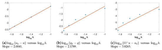
Figure 1. ${log}_{10}\mathrm{E}$ versus ${log}_{10}h$, where E is the L² error at T = 0.5 with P¹ basis.

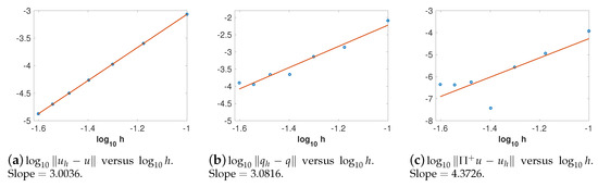
Figure 2. ${log}_{10}\mathrm{E}$ versus ${log}_{10}h$, where E is the L² error at T = 0.5 with P² basis.

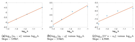
Figure 3. ${log}_{10}\mathrm{E}$ versus ${log}_{10}h$, where E is the L² error at T = 0.5 with P³ basis.

Next, we check the conservation properties of our schemes using a simulation over a long time. As indicated by Theorems 1 and 2 in Section 2.2, and Theorem 5 in Section 4, the conservation properties of energy and linear momentum are independent of the degree of polynomials. Here, we only present the long time simulation when $P^2$ basis is used. We still consider the initial-boundary value problem (73)–(75). We choose $h=0.1$, $\delta t={10}^{-4}$ and run the simulation up to $T=100$. Using the exact solution $u(x,t)=sin\left(2\pi x\right)cos\left(\sqrt{4{\pi }^2+1}t\right)$, we can show that the linear momentum $P\left(t\right)={\int }_I{u}_t{u}_{x}dx=0$ for all t. Numerically, we approximate the linear momentum using the discrete form of $P\left(t\right)$. That is, we compute ${\int }_I\left(u_h^{n+1}-u_h^n\right)/\delta t·q_h^{n+1}dx$ for $n=0,1,\dots ,{10}^6-1$, and present the time history of the error in linear momentum in Figure 4b. We can observe that the error oscillates from $T=0$ to $T=100$, and the magnitude of oscillations increase up to $T=76$ and then decrease from $T=76$ all the way to $T=100$. Overall, the linear momentum is conserved up to the magnitude of ${10}^{-10}$. Theorem 2 implies that the rate of change for linear momentum depends on some jumps at interior interfaces, and the semi-discrete form of linear momentum is not conserved up to machine epsilon. However, our numerical results indicate that the quantity ${\sum }_{j=1}^N|{\left[q_h\right]}_{j+\frac{1}{2}}{|}^2+{\sum }_{j=1}^N|{\left[u_h\right]}_{j+\frac{1}{2}}{|}^2-{\sum }_{j=1}^N{\left|{\left[u_{h,t}\right]}_{j+\frac{1}{2}}\right|}^2$, although not equal to zero analytically, is not far away from machine epsilon numerically. Therefore, we can observe the conservation of linear momentum numerically. As for the conservation of total energy, we compute the discrete form of energy using ${\int }_I{u}_h^{n+1}{u}_h^{n}dx+{\int }_I{q}_h^{n+1}{q}_h^{n}dx+{∥u_h^{n+1}-u_h^n∥}^2/{\left(\delta t\right)}^2$ for $n=0,1,\dots ,{10}^6-1$. Figure 4a shows the error in the total energy. We can observe that the total energy is conserved up to the magnitude of ${10}^{-9}$. Therefore, we have verified the energy conservation and linear momentum conservation through the numerical experiments.

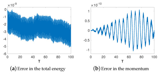
Figure 4. Time history of the error in the total energy and linear momentum with P² basis and h = 0.1. (left) error in the total energy; (right) error in the linear momentum.

6. Conclusions

In this paper, high-order energy and linear momentum conserving methods are proposed for the Klein-Gordon equation. Our numerical methods are based on the local discontinuous Galerkin methods. By choosing alternating numerical fluxes (6), we can prove that the total energy of the equation is exactly conserved and the linear momentum is conserved up to some terms at element interface. Results from long time numerical simulations (up to $T=100$) indicate that the linear momentum is conserved up to the magnitude of ${10}^{-10}$. Moreover, such a choice of numerical fluxes leads to optimal convergence order of $u_h$, $q_h$ and $u_{h,t}$, and the superconvergence property. It is important to mention that the schemes proposed in this paper can be directly generalized to the Klein-Gordon equation with external potential. Moreover, the results from this paper shed light on the design of high-order structure-preserving methods for nonlinear coupling systems involving the Klein-Gordon equation, for example, the Klein-Gordon-Schrödinger equations and the Klein-Gordon-Zakharov equations, which is currently under investigation.

References

- Ablowitz, M.J.; Kruskal, M.D.; Ladik, J.F. Solitary wave collisions. SIAM J. Appl. Math. 1979, 36, 428–437. [Google Scholar] [CrossRef]
- Fucito, F.; Marchesoni, F.; Marinari, E.; Parisi, G.; Peliti, L.; Ruffo, S.; Vulpiani, A. Approach to equilibrium in a chain of nonlinear oscillators. J. Phys. 1982, 43, 707–713. [Google Scholar] [CrossRef]
- Han, H.; Zhang, Z. Split local absorbing conditions for one-dimensional nonlinear Klein-Gordon equation on unbounded domain. J. Comput. Phys. 2008, 227, 8992–9004. [Google Scholar] [CrossRef]
- Jimenez, S. Comportamiento de Ciertas Cadenas de Osciladores No Lineales. Ph.D. Thesis, Universidad Complutense de Madrid, Madrid, Spain, 1988. [Google Scholar]
- Kirby, R.C.; Kieu, T. Galerkin finite element methods for nonlinear Klein-Gordon equations. Math. Comput. 2013. submitted. [Google Scholar]
- Yang, L. Numerical Studies of the Klein-Gordon-Schrödinger Equations. Master’s Thesis, National University Singapore, Singapore, 2006. [Google Scholar]
- Yin, F.; Tian, T.; Song, J.; Zhu, M. Spectral methods using Legendre wavelets for nonlinear Klein/Sine-Gordon equations. J. Comput. Appl. Math. 2005, 275, 321–334. [Google Scholar] [CrossRef]
- Li, S.; Vu-Quoc, L. Finite difference calculus invariant structure of a class of algorithms for the nonlinear Klein-Gordon equation. SIAM J. Numer. Anal. 1995, 32, 1839–1875. [Google Scholar] [CrossRef]
- Cockburn, B.; Hou, S.; Shu, C.W. TVB Runge-Kutta local projection discontinuous Galerkin finite element method for conservation laws IV: The multidimensional case. J. Comput. Phys. 1998, 141, 199–224. [Google Scholar] [CrossRef]
- Cockburn, B.; Lin, S.-Y.; Shu, C.-W. TVB Runge-Kutta local projection discontinuous Galerkin finite element method for conservation laws III: One dimensional systems. J. Comput. Phys. 1989, 84, 90–113. [Google Scholar] [CrossRef]
- Cockburn, B.; Shu, C.-W. TVB Runge-Kutta local projection discontinuous Galerkin finite element method for scalar conservation laws II: General framework. Math. Comput. 1989, 52, 411–435. [Google Scholar]
- Cockburn, B.; Shu, C.-W. TVB Runge-Kutta local projection discontinuous Galerkin finite element method for scalar conservation laws V: Multidimensional systems. Math. Comput. 1989, 52, 411–435. [Google Scholar]
- Xu, Y.; Shu, C.-W. Local discontinuous Galerkin methods for high-order time-dependent partial differential equations. Commun. Comput. Phys. 2010, 7, 1–46. [Google Scholar]
- Yan, J.; Shu, C.-W. A Local Discontinuous Galerkin Method for KdV-type Equations. SIAM J. Numer. Anal. 2002, 40, 769–791. [Google Scholar] [CrossRef]
- Yan, J.; Shu, C.-W. Local Discontinuous Galerkin Methods for Partial Differential Equations with Higher Order Derivatives. J. Sci. Comput. 2002, 17, 27–47. [Google Scholar] [CrossRef]
- Chou, C.-S.; Sun, W.; Xing, Y.; Yang, H. Local discontinuous Galerkin methods for the Khokhlov-Zabolotskaya-Kuznetzov equation. J. Sci. Comput. 2017, 73, 593–616. [Google Scholar] [CrossRef]
- Levy, D.; Shu, C.-W.; Yan, J. Local discontinuous Galerkin methods for nonlinear dispersive equations. J. Comput. Phys. 2004, 196, 751–772. [Google Scholar] [CrossRef]
- Xing, Y.; Chou, C.-S.; Shu, C.-W. Energy conserving local discontinuous Galerkin methods for wave propagation problems. Inverse Probl. Imaging 2013, 7, 967–986. [Google Scholar] [CrossRef]
- Xu, Y.; Shu, C.-W. Local discontinuous Galerkin methods for two classes of two-dimensional nonlinear wave equations. Phys. D Nonlinear Phenom. 2005, 208, 21–58. [Google Scholar] [CrossRef]
- Cheng, Y.; Christlieb, A.J.; Zhong, X. Energy-conserving discontinuous Galerkin methods for the Vlasov-Maxwell system. J. Comput. Phys. 2014, 279, 145–173. [Google Scholar] [CrossRef]
- Yang, H.; Li, F. Discontinuous Galerkin methods for relativistic Vlasov-Maxwell system. J. Sci. Comput. 2017, 73, 1216–1248. [Google Scholar] [CrossRef]
© 2018 by the author. Licensee MDPI, Basel, Switzerland. This article is an open access article distributed under the terms and conditions of the Creative Commons Attribution (CC BY) license (http://creativecommons.org/licenses/by/4.0/).