Rheological Behavior of Rockmass Supported with Rockbolts Based on Viscoelastic Analysis Method

Abstract

In this paper, we present the viscoelastic solutions for rockmass supported with discretely mechanically or frictionally coupled (DMFC) rockbolts to reveal the coupling rheological mechanisms. The analytical solutions are first acquired by applying the Laplace inverse transforms. The effect of different viscosity coefficients and supporting parameters on the coupling model rheological behavior are then investigated. It is concluded that the variation of the rockbolt axial force or rock mass stress and displacement have a close relationship with rheological parameters and support parameters. In addition, the variations of mechanical states of rockbolts and rock mass are closely related to the rheological model.

1. Introduction

Cavern excavations are necessary in underground resource exploitation and transport. A large number of laboratory tests and on-site monitoring indicate that the rock mass stress and displacement change have a significant time-dependence, which can cause not only the load of supporting structure but also the deformation to increase continuously [1,2,3,4], and it is easy for this to cause engineering deformation and instability damage to rock slopes, mine roadways, etc. Rockbolts, as an effective rock reinforcement measure, are widely applied in civil and mining engineering [5,6,7,8,9]. Unfortunately, the interaction mechanism of the rockbolt and ground is very complicated, and the coupling rheology mechanism of the rockbolt and rock mass is not well understood [10]. Field monitoring is obviously useful, but it can be complicated and expensive. Therefore, studying the time-dependent mechanism between the rock mass and rockbolt using a theoretical approach is meaningful.

The rockbolt belongs to a large support family, which was called the “rockbolt reinforcement system”, and the types of rockbolt reinforcement systems can be classified as (1) continuously mechanically coupled (CMC), (2) continuously frictionally coupled (CFC), and (3) discretely mechanically or frictionally coupled (DMFC) systems, and the classification is based on how the element load is transferred to the rock mass [8]. For the DMFC rockbolt reinforcement system, the interaction can be treated as two uniformly compressive distributed loads applied at both ends of the rock mass, and the rock mass is divided into two zones: respectively, the reinforced zone and original zone. In addition, the reinforced zone is simplified as homogeneous viscoelastic models [2,11,12,13].

Various approaches have been established to describe the rheological properties in rock mass based on analytical solutions [14,15,16], empirical approaches [17,18,19], and numerical methods [20,21,22]. Pan and Dong [23] treated the tunnel deformation as a time-dependent process, and applied the viscoelastic method to study the rheological features. Phienwej et al. [24] solved analytical solutions through the hyperbolic and power creep laws for predicting the time-dependent behavior of circular tunnels and found that the closure and support yielding time were most sensitive to the hyperbolic parameter and the creep parameter. Li et al. [25] explained the influence of stress, the creep coefficient and geometry parameters on the stress relaxation of bolts, but the rock mass rheological features were not mentioned. Hao Tang [26] studied a new four-element rock creep model based on variable-order fractional derivatives and continuum damage mechanics, so an important focus of research on rock creep has been to develop a model with few parameters and better simulation performance. Wang et al. [3] acquired the viscoelastic solutions of the circular tunnel supported with a pre-tensioned rockbolt using a distributed force model. However, the influence of a rockbolt without pretension force on rheological features was not involved, and the pretension will be weakened over time; the rheological features of a rock mass-supported DMFC rockbolt without pretension force should be investigated in depth.

In this paper, we begin by discussing the coupling model elastic solutions and then acquire the viscoelastic analytical solutions by Laplace reverse. Subsequently, we solve the analytical solutions with different rheological models. Finally, the changes in the rockbolt axial force, stress and deformation of rock mass with time are discussed through the analytical solutions.

2. Interaction Model

The relative distribution of the rockbolts and rock mass is shown in Figure 1. R is the radius of the reinforced zone, r is the radius of the circular cavern, $S_{\theta }$ is the interval of rockbolts along the tangential direction, and $S_Z$ is the interval of rockbolts along the tunnel axis direction. The following assumptions are made: (a) the cavern is deep and circular; (b) the problem is axisymmetric, and the lateral pressure coefficient K_a = 1; and (c) the deformation is minor. Given these assumptions, the analytical solutions are axisymmetric, and the solutions of various viscoelastic models can be obtained from the corresponding elastic solutions based on a standard procedure (the corresponding principle between elasticity and viscoelasticity) [27].

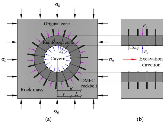
Figure 1. Geometric model of discretely mechanically or frictionally coupled (DMFC) rockbolts and rock mass: (a) plane direction; (b) excavation direction.

The internal structure of the interaction model is shown in Figure 2. In the interaction model, the displacement compatibility between the rockbolt and the rock mass can be expressed as Equation (1), where displacements of the rockbolt and rock mass are equaled at both ends of the rockbolt:

$$\begin{array}{l}{u_{\rho }|}_{\rho =r}={u_{\rho ,\mathrm{rockbolt}}|}_{\rho =r}\\ {u_{\rho }|}_{\rho =R}={u_{\rho ,\mathrm{rockbolt}}|}_{\rho =R}\end{array}\}$$

(1)

where u_ρ is the radial displacement of rock mass, u_ρ,rockbolt is the displacement of rockbolt, and ρ is radial distance. The interaction between rock mass and rockbolt can be expressed as

$$\begin{array}{l}{{\sigma }_{\rho }|}_{\rho =r}={\frac{1}{S_{\theta }{S}_Z}T|}_{\rho =r}\\ {{\sigma }_{\rho }|}_{\rho =R^{-}}-{{\sigma }_{\rho ,\mathrm{rock}}|}_{\rho =R^{+}}={\frac{r}{R{S}_{\theta }{S}_Z}T|}_{\rho =r}\end{array}\}$$

(2)

where σ_ρ is the radial stress of the rock mass, and T is the axial force of the rockbolt.

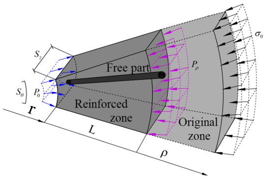
Figure 2. Internal structure of the interaction model.

Under the conditions described above, the problem is axisymmetric. In other words, stresses and displacements are independent of the polar coordinate $\theta$. In Figure 2, L is the length of the rockbolt free part, the mean supporting stress of rockbolts P₀ is distributed at the tunnel perimeter, and P_ρ where P_ρ = $r{P}_0/R$ at the rockbolt bond. When the rockbolt strain is $\epsilon$ and the axial stress is $\sigma$, the one-dimensional constitutive equation of rockbolt can be expressed as

$$T=A_C\sigma =A_C\frac{Q_C(D)}{P_C(D)}\epsilon$$

(3)

where T is the axial force of the rockbolt, A_C is the area of the rockbolt cross-section, D is the differential operator, t is time, p_k and q_k are both the constant parameters of the material, P(D) and Q(D) are the operator functions.

Then, the mean supporting stress P₀ that the rockbolts act on the tunnel wall is

$$P_0=\frac{T}{S_{\theta }{S}_Z}=\frac{A_C}{S_{\theta }{S}_Z}\frac{Q_C(D)}{P_C(D)}\epsilon =\frac{A_C}{S_{\theta }{S}_Z}\frac{Q_C(D)}{P_C(D)}\frac{\Delta L}{L}=k\Delta L=k\left[u_{\rho }\left(R\right)-u_{\rho }\left(r\right)\right]$$

(4)

where $u_{\rho }$ is the displacement of the rock mass in the radial direction, $\Delta L$ is the deformation of the rockbolt, and k is the equivalent stiffness of the rockbolt which can be expressed as

$$k=\frac{A_C}{S_{\theta }{S}_{Z}L}\frac{Q_C(D)}{P_C(D)}$$

(5)

When the constitutive model of the rockbolt is a one-dimensional Kelvin viscoelastic model, the operator functions of $Q_C\left(D\right)$ and $P_C\left(D\right)$ after Laplace transformation are

$$\begin{array}{l}\overline{P_C}\left(s\right)=1\\ \overline{Q_C}\left(s\right)=E_C+{\eta }_{C}s\end{array}\}$$

(6)

where $s$ represents the variable after Laplace transformation, ${\eta }_C$ is the viscosity coefficient of rockbolt, and $E_C$ is the Young’s modulus of the rockbolt.

When the constitutive model of the rockbolt is a one-dimensional Maxwell model, the operator functions of $Q_C\left(D\right)$ and $P_C\left(D\right)$ after Laplace transformation are

$$\begin{array}{l}\overline{P_C}\left(s\right)=1+\frac{{\eta }_C}{E_C}s\\ \overline{Q_C}\left(s\right)={\eta }_{C}s\end{array}\}$$

(7)

Using the generalized Hooke’s law, the following three-dimensional viscoelastic constitutive equation can be obtained from extending the one-dimensional constitutive equation:

$$\begin{array}{l}{S}_{ij}=2\frac{Q^{\prime }(D)}{P^{\prime }(D)}{e}_{ij}\\ {\sigma }_{ij}=3\frac{Q^{″}(D)}{P^{″}(D)}{\epsilon }_{ij}\end{array}\}$$

(8)

where $S_{ij}$ is the stress partial tensor, $e_{ij}$ is the strain partial tensor, ${\sigma }_{ij}$ is the stress tensor, and ${\epsilon }_{ij}$ is the strain tensor, $Q^{\prime }\left(D\right)$, and $P^{\prime }\left(D\right)$, $Q^{″}\left(D\right)$ and $P^{″}\left(D\right)$ are the operator functions of three-dimensional viscoelastic equation.

Under the condition of small deformation, the only difference between the elastic problem and viscoelastic problem lies in the constitutive equation. The equilibrium differential equation, geometric equation and boundary equation are all the same. Based on the elastic-viscoelastic principle, the solution of the viscoelastic problem can be obtained through the following procedure: (1) obtaining elastic solution and conducting Laplace transformation; (2) substituting viscoelastic parameters in the phase space into the elastic solutions, and then obtaining the Laplace space equations of the viscoelastic problem; and (3) obtaining the solution of the viscoelastic problem by Laplace inverse transformation [27]. The conversion formulae of the viscoelastic problem expressed in the phase space are shown as follows:

$$\begin{array}{l}\overline{E}(s)=\frac{9\overline{Q^{\prime }}(s)\overline{Q^{″}}(s)}{3\overline{P^{\prime }}(s)\overline{Q^{″}}(s)+\overline{P^{″}}(s)\overline{Q^{\prime }}(s)}\\ \overline{\mu }(s)=\frac{3\overline{P^{\prime }}(s)\overline{Q^{″}}(s)-2\overline{P^{″}}(s)\overline{Q^{\prime }}(s)}{2\left[3\overline{P^{\prime }}(s)\overline{Q^{″}}(s)+\overline{P^{″}}(s)\overline{Q^{\prime }}(s)\right]}\end{array}\}$$

(9)

where $\overline{E}(s)$ is elasticity modulus after Laplace transformation, $\overline{\mu }(s)$ is Poisson’s ratio after Laplace transformation, $\overline{Q^{\prime }}(s)$ $\overline{Q^{″}}(s)$ $\overline{P^{\prime }}(s)$ and $\overline{P^{″}}(s)$ are the forms of operator function $Q^{\prime }\left(D\right)$, $Q^{″}\left(D\right)$, and $P^{\prime }\left(D\right)$ and $P^{″}\left(D\right)$ are the forms after Laplace transformation.

When the constitutive model of rock mass is the Kelvin model, the three-dimension operator functions are

$$\overline{P^{\prime }}\left(s\right)=1$$

(10a)

$$\overline{Q^{\prime }}\left(s\right)=G_1+{\eta }_{2}s$$

(10b)

$$\overline{P^{″}}\left(s\right)=1$$

(10c)

$$\overline{Q^{″}}\left(s\right)=K$$

(10d)

where G₁ is the shear modulus of rock, K is the bulk modulus of rock, and η₂ is the rock mass viscosity coefficient.

When the constitutive model of rock mass is the Maxwell model, the equations of the operator functions in three dimensions are

$$\overline{P^{\prime }}\left(s\right)=1+{\eta }_{2}s/G_1$$

(11a)

$$\overline{Q^{\prime }}\left(s\right)={\eta }_{2}s$$

(11b)

$$\overline{P^{″}}\left(s\right)=1$$

(11c)

$$\overline{Q^{″}}\left(s\right)=K$$

(11d)

3. Viscoelastic Analytical Solutions in K–K Constitutive Model

The advantage of a closed-form solution is that the key variables that determine the ground-bolt response can be readily identified and their relative importance can be quickly estimated. For example, the formula derivation is provided when the constitutive model of rock mass and rockbolts is the K–K model. In order to obtain the viscoelastic interaction solutions of rock mass and rockbolts, the elastic coupling solution of rock mass and rockbolts must be obtained at first. The elastic solutions of the interaction model are shown in Appendix A [8,28].

Substituting the operator function $\overline{Q_C}\left(s\right)$, $\overline{P_C}\left(s\right)$, $\overline{Q^{\prime }}\left(s\right)$, $\overline{P^{\prime }}\left(s\right)$, $\overline{Q^{″}}\left(s\right)$, $\overline{P^{″}}\left(s\right)$ into Equations (5) and (9), we can obtain the conversion formulae of the K–K model. Then, substituting the K–K model conversion formulae into the elastic equations, as in Appendix A (A1)–(A6), we can obtain the Laplace space equations of the viscoelastic problem as in Appendix B (A7)–(A13).

The solutions of the rheological model of the DMFC rockbolt in circular tunnels can be derived from Appendix B (A7)–(A13) by the Laplace inverse transformation. The process is shown in Appendix C.

The viscoelastic solutions under an M–M model can be acquired by a similar method.

4. Analysis of Analytical Solutions

4.1. K-K Rheology Model

The input data for the rheological model for the rockbolt interaction are shown in Table 1.

Table 1. Experiment parameters.

Experiment No.	ηC (Pa·s)	EC (Pa)	η2 (Pa·s)	K (Pa)	G0 (Pa)	σ0 (Pa)	r (m)	R (m)	AC (m2)	L (m)	Sθ (m)	SZ (m)
A	1.0 × 1020	2.0 × 1011	1.0 × 1018	2.2 × 109	1.5 × 109	−3.0 × 106	4	8	3.0 × 10-4	4	0.6981	1
B	3.0 × 1020	2.0 × 1011	1.0 × 1018	2.2 × 109	1.5 × 109	−3.0 × 106	4	8	3.0 × 10-4	4	0.6981	1
C	3.0 × 1020	2.0 × 1011	1.0 × 1018	2.2 × 109	1.5 × 109	−3.0 × 106	4	8	3.0 × 10-4	4	1.0472	1
D	3.0 × 1020	2.0 × 1011	1.0 × 1018	2.2 × 109	1.5 × 109	−3.0 × 106	4	8	3.0 × 10-4	4	1.2566	1
E	3.0 × 1020	2.0 × 1011	1.0 × 1018	2.2 × 109	1.5 × 109	−3.0 × 106	4	8	3.0 × 10-4	4	0.5236	1
F	3.0 × 1020	2.0 × 1011	0.9 × 1018	2.2 × 109	1.5 × 109	−3.0 × 106	4	8	3.0 × 10-4	4	0.6981	1
G	3.0 × 1020	2.0 × 1011	1.1 × 1018	2.2 × 109	1.5 × 109	−3.0 × 106	4	8	3.0 × 10-4	4	0.6981	1
H	3.0 × 1020	2.0 × 1011	1.2 × 1018	2.2 × 109	1.5 × 109	−3.0 × 106	4	8	3.0 × 10-4	4	0.6981	1

The relationship between the axial force of the rockbolt and time under different viscosity coefficients ${\eta }_C$ is shown in Figure 3a. As shown in Figure 3c, the absolute value of the radial stress ${\sigma }_{\rho }$ at the position ρ = r equals the mean stress that rockbolts act on the tunnel walls. As the radial distance increases, the radial stress increases and slowly converges to the far-field stress ${\sigma }_0$. There is a jump in radial stress at the end of the rockbolt (ρ = R), and the radial stress (absolute value) in the reinforced zone $\underset{\rho \to R^{-}}{\lim }\left|{\sigma }_{\rho }\right|$ is larger than that in the original zone $\underset{\rho \to R^{+}}{\lim }\left|{\sigma }_{\rho }\right|$, and the jump value equals the distributed load at the end of rockbolt ($\underset{\rho \to R^{-}}{\lim }\left|{\sigma }_{\rho }\right|-\underset{\rho \to R^{+}}{\lim }\left|{\sigma }_{\rho }\right|=r{P}_0/R$). When ${\eta }_C=3\times {10}^{20} \mathrm{Pa}\cdot \mathrm{s}$, the numerical result of the radial stress in the reinforced zone decreases with time and then increases in the original zone. In addition, the jump value of the radial stress at the end of the rockbolt (ρ = R) decreases with time at ${\eta }_C=3\times {10}^{20} \mathrm{Pa}\cdot \mathrm{s}$, but increases at ${\eta }_C=1\times {10}^{20} \mathrm{Pa}\cdot \mathrm{s}$. When ${\eta }_C=1\times {10}^{20} \mathrm{Pa}\cdot \mathrm{s}$, the numerical value of the radial stress increases with time in the reinforce zone and the original zone. As shown in Figure 3d, the absolute value of the tangential stress ${\sigma }_{\theta }$ decreases with the radial distance. As the radial distance increases, the tangential stress ${\sigma }_{\theta }$ slowly converges to the far-field stress ${\sigma }_0$. At the end of the rockbolt ($\rho =R$), the tangential stress in the reinforced zone $\underset{\rho \to R^{-}}{\lim }\left|{\sigma }_{\theta }\right|$ is smaller than that in the original zone $\underset{\rho \to R^{+}}{\lim }\left|{\sigma }_{\theta }\right|$. In addition, the tangential stress (absolute value) in the reinforced zone increases with time and the viscosity coefficient of the rockbolt, but in the original zone, the tangential stress (absolute value) decreases. The variation of tangential stress increases with the viscosity coefficient in the original zone and decreases in the reinforced zone. As shown in Figure 4b, the displacement at time $t=0$ equals zero, and increases with time. The rock mass displacement decreases with the viscosity coefficient of the rockbolt.

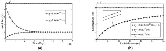
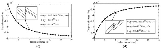
Figure 3. Mechanical states in experiments A and B. (a) Axial force–time curves; (b) Displacement–radial distance curves when the time equals zero or 6.0 × 10⁹ s; (c) Radial stress–radial distance curves when the time equals zero or 6.0 × 10⁹ s; (d) Tangential stress–radial distance curves when the time equals zero or 6.0 × 10⁹ s.

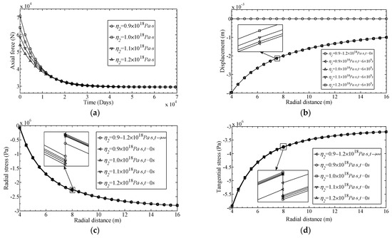
Figure 4. Mechanical states in experiments B, F, G and H. (a) Axial force–time curves; (b) Displacement–radial distance curves when the time equals zero or 6.0 × 10⁹ s; (c) Radial stress–radial distance curves when the time equals zero or 6.0 × 10⁹ s; (d) Tangential stress–radial distance curves when the time equals zero or 6.0 × 10⁹ s.

The results of experiments B, F, G and H are shown in Figure 4, and the variable among these experiments is the viscosity coefficient of the rock mass (${\eta }_2$). As shown in Figure 4a, the axial force of the rockbolt under different viscosity coefficients is exactly the same at time $t\to \infty$, because the displacement of the rock mass and rockbolts equals the elastic deformation at that time. A similar phenomenon also can be found in Figure 4b–d. When $t>0$, the axial force of the rockbolt increases with the viscosity coefficient of rock mass. As shown in Figure 4c, when $t>0$, the variation of the radial stress increases with the viscosity coefficient ${\eta }_2$ in the reinforced zone and decreases in the original zone. As shown in Figure 4d, the absolute value of the tangential stress in the reinforced zone increases with ${\eta }_2$, but decreases in the original zone. The displacement of rock mass is shown in Figure 4b; based on the comparison between the displacement–time relations under different viscosity coefficients ${\eta }_2$, we can see that the displacement decreases with the viscosity coefficient ${\eta }_2$.

The results of experiments B, C, D and E are shown in Figure 5, and the variable among these experiments is the intersection angle of the rockbolts (the spacing of rockbolts along the tangential direction, $S_{\theta }$). Compared with results of experiments B, F, G and H, the most significant differences are that the axial force of the rockbolt, the radial stress and tangential stress of the rock mass, and the displacement in the rock mass are not constant for different spacings of rockbolts at $t\to \infty$, and these values are determined by the spacing of the rockbolts. As shown in Figure 5a, the axial force of a rockbolt increases with the intersection angle of the rockbolts. As shown in Figure 5c, the absolute value of the radial stress increases with the intersection angle of the rockbolts in the reinforced zone, but decreases in the original zone. As shown in Figure 5d, the absolute value of the tangential stress in the reinforced zone decreases with the intersection angle of rockbolts, but increases in the original zone. As shown in Figure 5b, the displacement of rock mass increases with the intersection angle of the rockbolts. The results from the experiments B, C, D and E indicate that the reinforcement effect of rockbolts decreases with the intersection angle.

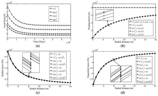
Figure 5. Mechanical states in experiments B, C, D and E. (a) Axial force–time curves; (b) Displacement–radial distance curves when the time equals zero or 6.0 × 10⁹ s; (c) Radial stress–radial distance curves when the time equals zero or 6.0 × 10⁹ s; (d) Tangential stress–radial distance curves when the time equals zero or 6.0 × 10⁹ s.

4.2. Different Constitutive Models for Rock Mass and Rockbolts

Using a similar methodology for the analytical solutions of the K–K model, the analytical solutions of the M–M model can be obtained. The mechanical behaviors of the M–M model are extremely different from those of the K–K model. For example, when using the M–M model, the displacements of the rock mass and rockbolts equals the corresponding elastic solutions at $t=0$, and always increase with time. The deformation velocity decreases with time and tends to keep constant finally. There is no limitation in the displacements of the rock mass and rockbolt in the M–M model. However, for the case of the K–K model, the displacement equals zero at $t=0$ and increases with time. The ultimate deformation of rock mass or rockbolts equals the corresponding elastic problem solutions (also equalling the displacement obtained from the M–M model at $t=0$). The deformation velocity decreases with time and eventually reduces to zero.

For the case of the M–M model, the variation of the axial force is related to the viscosity coefficient of rockbolts ${\eta }_C$. In a certain range, the axial force increases with time and gradually reaches its peak value when the viscosity coefficient of the rockbolts is larger than a certain value (the curve in Figure 6, M–M model, ${\eta }_C=3\times {10}^{20} \mathrm{Pa}\cdot \mathrm{s}$). In contrast, the axial force decreases with time and reaches its minimum value (the curve in Figure 6, K–K model, ${\eta }_C=1\times {10}^{20} \mathrm{Pa}\cdot \mathrm{s}$). As shown in Figure 6, the characteristics between the axial force of the rockbolt and the viscosity coefficient of the K–K model are opposite to those of the M–M model. The variation of the axial force of the rockbolt shows an opposite pattern between the M–M model and the K–K model for the same parameters.

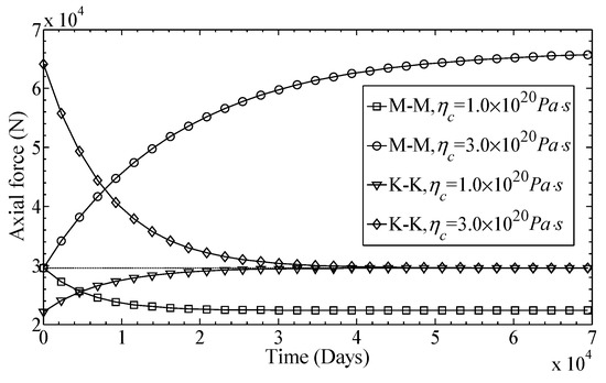
Figure 6. Axial force–time curves obtained from M–M model and K–K model with different viscosity coefficients of rockbolts.

As shown in Figure 7, these displacement–time curves represent the displacement of surrounding rock mass at the position $\rho$ = 4 m under the condition of the M–M model and K–K model; the different variable used in these curves is the viscosity coefficient of rock mass. In Figure 8, the curves also represent the displacement of the rock mass at the position $\rho$ = 4 m under the condition of the M–M model and the K–K model, but the different variable between these curves is the viscosity coefficient of the rockbolt. It can be seen from Figure 7 and Figure 8, the displacements obtained from the M–M model and the K–K model increase with time. The displacement obtained from the M–M model equals the corresponding elastic solution at $t=0$ and increases with time. However, the displacement obtained from the K–K model equals zero at $t=0$, and the ultimate displacement equals the corresponding elastic solution. Therefore, the displacement obtained from the M–M model at $t=0$ equals that from the K–K model at $t\to \infty$. In Figure 7, as the viscosity coefficient of the rock mass increases, the deformation velocity decreases, and the displacement of the surrounding rock mass in the M–M model is reduced. However, this does not affect the ultimate displacement obtained from the K–K model. In Figure 8, as the viscosity coefficient of the rockbolt increases, the displacement of the rock mass in the M–M model decreases, and the ultimate displacement obtained from the K–K model is impacted.

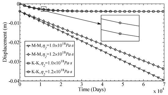
Figure 7. Displacement–time curves obtained from the M–M model and K–K model with different viscosity coefficients of rock mass.

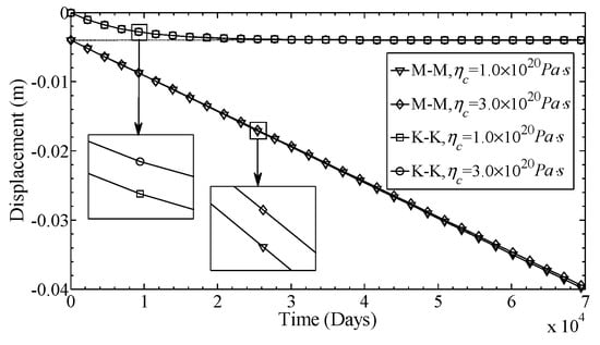
Figure 8. Displacement–time curves obtained from the M–M model and K–K model with different viscosity coefficients of rockbolts.

5. Conclusions

In this paper, an interaction rheological model of rockbolt and rock mass is proposed based on the reinforcement mechanism of DMFC rockbolts, and the long-term evolution of stress and displacement of the rock mass and rockbolts are discussed. The main conclusions can be drawn as follows:

(1)

Based on this study, the time-dependent features of rock mass–rockbolt rheology coupling is considered in the long-term design and maintenance of caverns, and the theoretical model can be used to evaluate the rheological mechanical properties of the interaction between the rock mass and DMFC rockbolts, and then the long-term mechanical behavior of the rockbolt supporting system can be predicted;

(2)

The evolution of the axial force of a rockbolt is closely related to the viscosity coefficient of rockbolts ${\eta }_C$. When using the M–M model, if ${\eta }_C$ is larger than a certain value ($T^{\prime }\left(t\right)>0$), the axial force of rockbolts increases with time, and eventually approaches a limit value. Conversely, the axial force decreases with time, and gradually approaches a minimum value. When using the K–K model, the variation of the axial force is opposite to the result from the M–M model. If the ${\eta }_C$ is larger than a certain value, the axial force decreases with time, and eventually approaches the corresponding elastic solution. In contrast, the axial force increases with time, and approaches the value of the corresponding elastic solution. In addition, when the viscosity coefficient of a rockbolt is relatively large, the axial force of the rockbolt may increase at first and then decrease;

(3)

The results show a marked difference when the Kelvin model is used as opposed to the Maxwell model; the reason for the difference is that the properties of these two models are different. The Maxwell model can describe the materials’ transient, relaxation and viscous flow, while the Kelvin model can only describe the elastic after-effect and deformation limit;

(4)

In this study, analytical solutions of the theoretical model under the circumstances of the K–K model and M–M model are given. This solution derivation methodology may also be applied to other types of rheological models; for example, the reasonable and simplified method for the theoretical model of a CFC rockbolt can be further studied based on this model, which lays a foundation of the preliminary research for solving the theoretical model of a CFC rockbolt. Additional details regarding rockbolt and rock mass coupling properties should be investigated using the appropriate rheological models in future work. Furthermore, the coupling model nonlinear viscoelastic behavior is also the next work.

References

- Sharifzadeh, M.; Abolfazl, T.; Mohammad, A.M. Time-dependent behavior of tunnel lining in weak rock mass based on displacement back analysis method. Tunn. Undergr. Space Technol. 2013, 38, 348–356. [Google Scholar] [CrossRef]
- Zhu, W.S.; Zhao, J. Stability Analysis and Modelling of Underground Excavations in Fractured Rocks; Elsevier Science: Amsterdam, The Netherlands, 2004. [Google Scholar]
- Wang, G.; Liu, C.Z.; Jiang, Y.J.; Wu, X.Z.; Wang, S.G. Rheological Model of DMFC Rockbolt and Rockmass in a Circular Tunnel. Rock Mech. Rock Eng. 2015, 48, 2319–2357. [Google Scholar] [CrossRef]
- Sun, J. Rock rheological mechanics and its advance in engineering applications. Chin. J. Rock Mech. Eng. 2007, 26, 1081–1106. [Google Scholar]
- Evert, H.; Ted, B. Underground Excavations in Rock; CRC Press: London, UK, 1980. [Google Scholar]
- Stillborg, B. Professional Users Handbook for Rock Bolting; Trans Tech Publications: Stafa-Zurich Switzerland, 1994. [Google Scholar]
- Windsor, C.R. Rock reinforcement systems. Int. J. Rock Mech. Min. Sci. 1997, 34, 919–951. [Google Scholar] [CrossRef]
- Bobet, A.; Einstein, H.H. Tunnel reinforcement with rockbolts. Tunn. Undergr. Space Technol. 2011, 26, 100–123. [Google Scholar] [CrossRef]
- Li, C.; Stillborg, B. Analytical models for rock bolts. Int. J. Rock Mech. Min. Sci. 1999, 36, 1013–1029. [Google Scholar] [CrossRef]
- Cai, Y.; Tetsuro, E.; Jiang, Y.J. A rock bolt and rock mass interaction model. Int. J. Rock Mech. Min. Sci. 2004, 41, 1055–1067. [Google Scholar] [CrossRef]
- Zhang, Y.J.; Liu, Y.P. 3D viscoelastic-viscoplastic FEM analysis for bolted orthotropic rockmass. Chin. J. Rock Mech. Eng. 2002, 21, 1770–1775. [Google Scholar]
- Zhu, Z.D. Rheologic analysis of action mechanism of underground roadway bolts. J. Shandong Univ. Sci. Technol. 1997, 16, 148–153. [Google Scholar]
- Wu, G.J.; Chen, W.Z.; Wang, Y.G. Study of distribution and variation of anchor stress based on creep effect of rock mass. Rock Soil Mech. 2010, 31, 150–155. [Google Scholar]
- Goodman, R. Introduction to Rock Mechanics, 2nd ed.; Wiley: New York, NY, USA, 1989. [Google Scholar]
- Nomikos, P.; Rahmannejad, R.; Sofianos, A. Supported axisymmetric tunnels within linear viscoelastic Burgers rocks. Rock Mech. Rock Eng. 2011, 44, 553–564. [Google Scholar] [CrossRef]
- Ladanyi, B.; Gill, D. Tunnel lining design in creeping rocks. In Proceedings of the Symposium on Design and Performance of Underground Excavations ISRM, Cambridge, UK, 3–6 September 1984. [Google Scholar]
- Sulem, J.; Panet, M.; Guenot, A. An analytical solution for time-dependent displacements in circular tunnel. Int. J. Rock Mech. Min. Sci. Geomech. Abstr. 1984, 24, 155–164. [Google Scholar] [CrossRef]
- Ladanyi, B. Time dependent response of rock around tunnel. In Comprehensive Rock Engineering: Principles, Practice & Projects; Hudson, J., Ed.; Pergamon Press: Oxford, UK, 1999; Volume 2, pp. 77–112. [Google Scholar]
- Panet, M. Understanding deformations in tunnels. In Comprehensive Rock Engineering: Principles, Practice & Projects; Hudson, J., Ed.; Pergamon Press: Oxford, UK, 1993; Volume 2, pp. 663–690. [Google Scholar]
- Ghaboussi, J.; Gioda, G. On the time-dependent effects in advancing tunnels. Int. J. Numer. Methods Geomech. 1977, 2, 249–269. [Google Scholar] [CrossRef]
- Gioda, G. A finite element solution of non-linear creep problems in rock. Int. J. Rock Mech. Sci. Geomech. Abstr. 1981, 8, 35–46. [Google Scholar] [CrossRef]
- Peila, D.; Oreste, P.; Rabajuli, G.; Trabucco, E. The pre-tunnel method, a new Italian technology for full-face tunnel excavation: A numerical approach to design. Tunn. Undergr. Space Technol. 1995, 10, 367–374. [Google Scholar] [CrossRef]
- Pan, Y.W.; Dong, J.J. Time-dependent tunnel convergence—I. Formulation of the model. Int. J. Rock Mech. Min. Sci. Geomech. Abstr. 1991, 28, 469–475. [Google Scholar] [CrossRef]
- Phienwej, N.; Thakur, P.K.; Cording, E.J. Time-dependent response of tunnels considering creep effect. Int. J. Geomech. 2007, 7, 296–306. [Google Scholar] [CrossRef]
- Li, J.J.; Zheng, B.L.; Xu, C.Y. Numerical analyses of creep behavior for prestressed anchor rods. Chin. Q. Mech. 2007, 28, 124–128. [Google Scholar]
- Tang, H.; Wang, D.P.; Huang, R.Q.; Pei, X.J.; Chen, W.L. A new rock creep model based on variable-order fractional derivatives and continuum damage mechanics. Bull. Eng. Geol. Environ. 2018, 77, 375–383. [Google Scholar] [CrossRef]
- Wang, Z.Y.; Li, Y.P. Rock Rheology Theory and Numerical Simulation; Beijing Science Press: Beijing, China, 2008. [Google Scholar]
- Kovári, K. History of the sprayed concrete lining method—Part I: Milestones up to the 1960s. Tunn. Undergr. Space Technol. 1992, 18, 57–69. [Google Scholar] [CrossRef]
© 2018 by the authors. Licensee MDPI, Basel, Switzerland. This article is an open access article distributed under the terms and conditions of the Creative Commons Attribution (CC BY) license (http://creativecommons.org/licenses/by/4.0/).