Nonparametric Functional Least Absolute Relative Error Regression: Application to Econophysics

Abstract

In this paper, we propose an alternative kernel estimator for the regression operator of scalar response variable S given a functional random variable T that takes values in a semi-metric space. The new estimator is constructed through the minimization of the least absolute relative error (LARE). The latter is characterized by its ability to provide a more balanced and scale-invariant measure of prediction accuracy compared to traditional standard absolute or squared error criterion. The LARE is an appropriate tool for reducing the influence of extremely large or small response values, enhancing robustness against heteroscedasticity or/and outliers. This feature makes the LARE suitable for functional or high-dimensional data, where variations in scale response are common. The high feasibility and strong performance of the proposed estimator are supported theoretically by establishing its stochastic consistency. The latter is derived with precision of the convergence rate under mild regularity conditions. The ease implementation and the stability of the estimator are justified by simulation studies and an empirical application to near-infrared (NIR) spectrometry data. Of course, to explore the functional architecture of this data, we employ random matrix theory (RMT), which is a principal analytical tool of econophysics.

1. Introduction

Examining how a functional predictor co-varies with a scalar response variable is a fundamental issue in functional statistics. This relationship is commonly evaluated through regression models, which is estimated using the least squares loss function. In this paper, we adopt another smoothing approach based on the least absolute relative error (LARE). Undoubtedly, the LARE criterion improves the robustness and the accuracy of the standard regression approaches.

The general framework of this paper is the nonparametric prediction in functional statistics, which has attracted considerable interest due to numerous valuable contributions in recent years. The foundational work in this field was introduced by [1], who established the almost complete pointwise consistency of the kernel-type regression estimator under the assumption of independent and identically distributed (i.i.d.) observations. Ref. [2] proved the convergence of this estimator in the $L^p$ norm. Ref. [3] derived the exact asymptotic expression for the corresponding $L^p$ errors. The asymptotic normality of the same estimator in the strong mixing case was later demonstrated by [4]. In addition to these classical kernel-based approaches, recent research has explored M-estimation techniques and/or local linear smoothing methods. Significant results in the field of nonparametric functional prediction were presented by [5,6], which provide comprehensive references on this topics.

Alternatively, in this paper, we focus on relative error regression (RE regression), a methodology in which the the relative error is used. The latter constitutes a performance measure in many practical applications. Despite its utility, the literature on nonparametric RE regression remains limited, since most existing studies adopted the parametric approaches. In this context, the authors of [6] were among the first to investigate the use of relative squared error in estimation. From a practical point of view, RE regression has been applied in diverse fields, including medicine [7] and finance [8]. In [9], authors studied estimation via RE regression in multiplicative regression models, while [10] extended this framework to nonparametric estimation, establishing the convergence of the local linear estimator derived from relative error loss.

In the last decade, RE regression has been explored extensively for dependent data. For instance, ref. [11] considered spatial time series, The functional nonparametric RE regression was first introduced by [12], who established strong consistency and derived the asymptotic distribution of the RE regression estimator. Ref. [13] extended the method to incomplete functional data, examining kernel smoothing techniques for truncated observations. For a comprehensive overview of the latest progress on this topic, see [14,15].

While all the cited studies estimate the regression operator using the mean least squares relative error (LSRE) loss function, in the present study, we adopt the absolute relative error loss function and integrate it with kernel-based local weighting approaches to construct a robust estimator for nonparametric functional regression. This so-called LARE regression improves the LSRE model [13,14] in terms of both robustness and estimation accuracy. Such gains are particularly valuable in functional data analysis, where observations are often contaminated by noise and characterized by high variability and high frequency. In functional setting, extreme observations and local variations frequently arise and can exert an excessive influence on estimation quality when LSRE is used. Unlike LSRE, the LARE regression treats deviations in a proportional manner, thereby reducing sensitivity to outliers. As a result, the proposed estimator yields more stable and reliable inference on the underlying functional relationship. This property makes LARE regression more suitable for high-frequency data and highly relevant in many applied fields, such as economics, finance, signal processing, and environmental sciences.

From a theoretical perspective, the analysis of the LARE regression model is considerably more complicated than that of the LSRE model. While the LSRE estimator admits an explicit representation in terms of ratios of inverted conditional moments, no such closed-form expression is available for the LARE estimator. Consequently, its asymptotic behavior must be established through a detailed Bahadur-type representation. Despite these analytical challenges, we prove the almost complete convergence of the proposed estimator and precisely characterize its rate of convergence under standard assumptions in nonparametric functional regression. These conditions reflect both the functional nature of the covariates and the structure of the model. An additional strength of LARE regression compared with LSRE regression is its wider range of applicability. While LSRE methods are restricted to strictly positive response variables, LARE regression removes this limitation and thereby extends the scope of potential applications. Finally, the practical relevance of the proposed estimator is illustrated through a data-driven approach for selecting the tuning parameter. In addition, comprehensive simulation studies and real-data analyses are conducted, all of which confirm the robustness and superior empirical performance of the proposed method.

This paper is organized as follows. In Section 2, we introduce the proposed estimation algorithms. Section 3 presents the required assumptions and the main asymptotic results. In Section 4, we discuss methods for selecting the smoothing parameter and the metric using the random matrix theory from econophysics. The performance of the constructed estimator on simulated and real data is evaluated in Section 5. Finally, Section 6 is devoted to summarize some concluding remarks. The technical proofs are provided in Appendix A.

2. Functional LARE Regression and Its Estimation

As outlined in the Introduction, our main objective is to evaluate the relationship between an exogenous functional variable T and a real-valued endogenous variable S. More precisely, the variables under consideration belong to the space $\mathcal{X}\times \mathrm{I}\mathrm{R}$. The set $\mathcal{X}$ is a functional space endowed with an appropriate semi-norm N. Henceforth, we fix a point $\mathcal{T}$ in $\mathcal{X}$ and consider a neighborhood ${\mathcal{N}}_{\mathcal{T}}$ of $\mathcal{T}$ within this functional space. In our earlier contributions [12], we modeled the underlying relationship between T and S using the LSRE regression defined by

$$\begin{array}{c}\hfill REG\left(\mathcal{T}\right)=arg\underset{s}{min}\mathrm{I}\mathrm{E}\left({\left({\displaystyle \frac{S-s}{S}}\right)}^2|T=\mathcal{T}\right).\end{array}$$

The main feature of this loss function is its ability to provide an explicit definition of the predictor. Indeed, by simple differentiation with respect to s, we can show that

$$REG\left(\mathcal{T}\right))={\displaystyle \frac{\mathrm{I}\mathrm{E}\left[S^{-1}|T=\mathcal{T}\right]}{\mathrm{I}\mathrm{E}\left[S^{-2}|T=\mathcal{T}\right]}}.$$

(1)

Thus, the LSRE regression can be explicitly expressed as the ratio of the first and second inverse moments. This explicit formulation of the model simplifies both the analysis and the derivation of its mathematical properties. Nevertheless, this approach is not without limitations. While the least squares relative error method reduces the effect of large outliers values, it can give excessive weight to large deviations, which compromised its robustness against the very small values or highly dispersed observations. To address this limitation, we propose to proceed with the least absolute relative error (LARE) approach, which provides a more balanced treatment of both small and large deviations in the data. Formally, the LARE regression is defined as the estimator that minimizes

$$\begin{array}{c}\hfill RER\left(\mathcal{T}\right)=arg\underset{s}{min}\mathrm{I}\mathrm{E}\left(\left|{\displaystyle \frac{S-s}{S}}\right||T=\mathcal{T}\right).\end{array}$$

(2)

Compared to (1), this alternative loss function enhances the robustness of LSRE regression by treating all deviations proportionally in a linear manner, rather than using the traditional quadratic form. The LARE loss function evaluates the differences between predicted and true values more equitably, providing a more balanced, resilient, and reliable assessment of model performance. This advantage is particularly important in the presence of large deviations or extremely small observations, where the LSRE approach fails to handle. Overall, the LARE rule is more robust and effective, especially in datasets with irregular or heavy-tailed distributions.

For the estimation setup, we consider n independent and identically distributed (i.i.d.) pairs, $(T_1,S_1),\dots ,(T_n,S_n)$, sampled from the distribution of $(T,S)$. The kernel estimator of $RER\left(\mathcal{T}\right)$ is then given by

$${\displaystyle \widehat{RER}\left(\mathcal{T}\right)=arg\underset{s}{min}\frac{{\sum }_{i=1}^{n}M\left(m^{-1}N(\mathcal{T},T_i)\right)\left|\frac{S_i-s}{S_i}\right|}{{\sum }_{i=1}^{n}M\left(m^{-1}N(\mathcal{T},T_i)\right)},}$$

(3)

where M is a kernel function and $m:=m_n$ (to simplify the notation) is a sequence of positive real numbers that goes to zero as n goes to infinity.

The primary objective of this paper is to establish the asymptotic properties of the estimator $\widehat{RER}\left(\mathcal{T}\right)$ of $RER\left(\mathcal{T}\right)$, where the explanatory variable T takes values in a semi-metric space $\mathcal{X}$. To the best of our knowledge, this work is the first to employ this approach to construct an estimator of the regression operator, even in multivariate settings. Although the finite-dimensional case can be viewed as a special case of this framework, the infinite-dimensional case is especially interesting, for both its theoretical challenges and the variety of practical applications it supports. For further motivation and detailed discussions on this topic, we refer the reader to [16,17,18] and the references therein.

3. The Strong Consistency of the Kernel Estimator

Now, to investigate the almost complete convergence, we denote by C or $C^{\prime }$ strictly positive constants and put

$$M_i=M\left(m^{-1}N(\mathcal{T},T_i)\right),i=1,\dots ,n.$$

We define the closed ball of radius r centered at $\mathcal{T}$ as

$$B(\mathcal{T},r)=\left\{\mathcal{Z}\in \mathcal{X}:N(\mathcal{Z},\mathcal{T})<r\right\},$$

and set

$$U_1(s,\mathcal{T})={\mathbb{E}[|S|}^{-1}1{\mathrm{I}}_{S\le s}\mid T=\mathcal{T}],U_2(s,\mathcal{T})={\mathbb{E}[|S|}^{-1}1{\mathrm{I}}_{S\ge s}\mid T=\mathcal{T}].$$

The following assumptions are imposed:

• (HM1) The small-ball probability satisfies $\mathbb{P}(X\in B(\mathcal{T},r))=:{\mathcal{G}}_{\mathcal{T}}\left(r\right)>0$ for all $r>0$, with

  $$\underset{r\to 0}{lim}{\mathcal{G}}_{\mathcal{T}}\left(r\right)=0.$$
• (HM2) For all ${\mathcal{T}}_1,{\mathcal{T}}_2\in {\mathcal{V}}_{\mathcal{T}}$, the functions $U_{\gamma }$ are of class $C^1$ (with respect to s) and satisfy

  $$|U_{\gamma }(s,{\mathcal{T}}_1)-U_{\gamma }(s,{\mathcal{T}}_2)| \le C{d}^{b_{\gamma }}({\mathcal{T}}_1,{\mathcal{T}}_2),b_{\gamma }>0,\gamma =1,2..$$
• (HM3) The kernel M is measurable, supported on $(0,1)$, and bounded: $0<C_2\le M(·)\le C_3<\infty$.
• (HM4) The small-ball probability satisfies

  $${\displaystyle \frac{n{\mathcal{G}}_{\mathcal{T}}\left(m\right)}{logn}}\to \infty \mathrm{as}n\to \infty .$$
• (HM5) The response variable is bounded by inverse moments,

  $$\forall p\ge 2,\mathbb{E}[S^{-p}\mid T=\mathcal{T}]<C(p,\mathcal{T})<\infty \mathrm{a}\mathrm{l}\mathrm{m}\mathrm{o}\mathrm{s}\mathrm{t} \mathrm{s}\mathrm{u}\mathrm{r}\mathrm{l}\mathrm{y}.$$

Discussion of the Assumptions

These assumptions are relatively mild and commonly used functional data analysis. The functional component is characterized by two main conditions. The first one is (HM1) and concerns the small-ball probability function, which describes the concentration behavior of the probability measure associated with the functional regressor. Assumption (HM1) plays a crucial role in controlling the dispersion term in the convergence rate. The nonparametric component is specified through assumption (HM2), which is standard in nonparametric functional statistics and has been used in several related studies. This assumption is employed to assess the bias term in the convergence rate. In addition, assumptions (HM3) and (HM4) impose technical conditions that facilitate the proofs and ensure the establishment of the claimed asymptotic results. Finally, assumption (HM5) is a classical condition in regression analysis for establishing almost complete consistency (see [19]). As expected, this condition is stronger than the finite-variance assumption and sufficient for convergence in probability. Since almost complete consistency represents a stronger mode of convergence, it naturally requires correspondingly stronger assumptions. Overall, the relationship between assumptions and results reflects a trade-off between generality and strength: stronger and more comprehensive results require correspondingly stronger assumptions.

Theorem 1.

Given assumptions (HM1)–(HM5), we obtain

$$|\widehat{RER}\left(\mathcal{T}\right)-RER\left(\mathcal{T}\right)\left)\right|=O\left(m^{b_1}\right)+O\left(m^{b_2}\right)+O_{a.co.}\left(\sqrt{{\displaystyle \frac{logn}{n{\mathcal{G}}_{\mathcal{T}}\left(m\right)}}}\right).$$

(4)

Note that the expression of the convergence rate confirms the statements discussed for previous assumptions. We observe that the first component of the convergence rate depends strongly on the constants $b_1$ and $b_2$, which are introduced in assumption (HM2) and characterize the functional space of the model. In contrast, the small-ball probability function ${\mathcal{G}}_{\mathcal{T}}\left(m\right)$ specified in assumption (HM1) appears in the second component, which captures the dispersion term of the convergence rate.

Now, the proof of this theorem employs the Bahadur representation of the $\widehat{RER}$ estimator. This representation is established through the following auxiliary results.

Lemma 1.

Let $\left\{{\mathcal{U}}_n\right\}$ be a sequence of decreasing real-valued random functions and $\left\{{\mathcal{D}}_n\right\}$ a real random sequence satisfying

$$\begin{array}{cc}\hfill {\mathcal{D}}_n& \stackrel{a.co.}{\to }0,\hfill \\ \hfill \underset{\left|d\right|\le A}{sup}\left|{\mathcal{U}}_n\left(d\right)+\beta d-{\mathcal{D}}_n\right|& \stackrel{a.co.}{\to }0,\hfill \end{array}$$

for some constants $\beta ,A>0$. Then, for any real random sequence $d_n$ such that ${\mathcal{U}}_n\left(d_n\right)\stackrel{a.co.}{\to }0$, we have

$$\sum _{n=1}^{\infty }\mathbb{P}\left(|d_n| \ge A\right)<\infty .$$

4. Smoothing Parameter Selection and Random Matrix Theory for Metric Approximation

The practical performance of the estimator $\tilde{R}$ depends crucially on the choice of parameters involved in its construction. In particular, the bandwidth parameter m plays a central role in the implementation of this regression method. Various strategies have been proposed in the nonparametric regression literature to address this issue. In this study, we adopt two widely used approaches from classical regression: the cross-validation rule and the bootstrap algorithm.

4.1. Leave-One-Out Cross-Validation Principle

In regression analysis, the leave-one-out cross-validation (LOOCV) criterion is based on minimizing the mean squared error. This criterion is highly effective for bandwidth selection because it directly optimizes for predictive accuracy. The LOOCV algorithm was successfully extended to the domain of functional statistics by [19] who demonstrated its particular efficacy and suitability for functional data. The main advantage of this approach is its flexibility; for instance, it can be readily adapted to our model for functional LARE regression as

$$m^{opt}=arg\underset{m\in \mathcal{M}}{min}\sum _{i=1}^n\left|{\displaystyle \frac{(S_i-{\widetilde{RER}}^{-i}\left(T_i\right))}{S_i}}\right|,$$

(5)

where ${\widetilde{RER}}^{-i}\left(T_i\right)$ and ${\widehat{RER}}^{-i}\left(T_i\right)$ denote the leave-one-out estimators of $RER$, respectively, computed without the i-th observation $(T_i,S_i)$. The efficiency of these estimators depends on the choice of the subset $\mathcal{M}$, which determines the optimization of (5).

Concerning the subset $\mathcal{M}$, we point out that there are two primary strategies for choosing it; the local approach and the global one. In the local case, $\mathcal{M}$ is determined by the number of neighborhoods around the location point. In the global case, $\mathcal{M}$ is derived from the quantiles of the distance distribution between the functional regressors.

4.2. Bootstrap Approach

The bootstrap procedure is an alternative popular method to the cross-validation rule. Its principal feature is its data-driven nature, as it empirically approximates the sampling distribution of the estimator without external assumptions. This automatism analysis makes it particularly valuable in complex modeling scenarios, where asymptotic theory may be intractable or slow to converge. Furthermore, the bootstrap provides a direct and computationally feasible means to minimize a targeted loss function. This allows for a more adaptive approach for many loss functions. For the LARE regression, we state the following algorithm:

• Step 1: Choose an arbitrary bandwidth $m_0$ and compute ${\widehat{RER}}_{m_0}\left(\mathcal{T}\right)$.
• Step 2: Compute the residual $\widehat{ϵ}=S-{\widehat{RER}}_{m_0}\left(\mathcal{T}\right)$.
• Step 3: Generate a bootstrap residual ${ϵ}^{*}$ using the distribution $G^{*}=((\sqrt{5}+1)/2\sqrt{5})d_{\widehat{ϵ}(1-\sqrt{5})/2}$$-((1-\sqrt{5})/2\sqrt{5})d_{\widehat{ϵ}(\sqrt{5}+1)/2}$, (d is dirac measure).
• Step 4: Construct a bootstrap sample ${(S_i^{*},T_i^{*})}_i=({ϵ}^{*}-{\widehat{RER}}_{m_0}\left(T_i\right)$.
• Step 5: Compute the estimators ${\widehat{RER}}_m\left(\mathcal{T}\right)$ using the sample ${(S_i^{*},T_i^{*})}_i$.
• Step 6: Repeat the steps 3–6 $N_B$ times and put ${\widehat{RER}}_m^r\left(\mathcal{T}\right)$ as the estimator at the replication r.
• Step 7: Choose the optimal bandwidth m according to the following criterion

  $$m_{op{t}^{Boo}}=arg\underset{m}{min}\sum _{r=1}^{N_B}\sum _{i=1}^n|{\widehat{RER}}_{m_0}\left(T_i\right)-{\widehat{RER}}_m\left(T_i\right)|.$$

4.3. Random Matrix Metric

The principal task of functional data analysis is to move from comparing two curves directly to compare them within the context of a larger noisy system. In this context, random matrix theory (RMT) is used to define a stable distance (without noise) between any two curves by eliminating the noise of the entire system. The main idea is based on the use of RMT to clean the covariance matrix estimated from the data. The eigenvalues and eigenvectors of the noisy covariance matrix are a mixture of true signal and random noise. RMT provides a null model to identify which parts of the spectrum are likely to be a noisy signal. To do that, we follow the following algorithm:

• Step 1: Create the sample covariance matrix

  $$\mathbf{C}={\displaystyle \frac{1}{n}}{\mathbf{T}}^{tr}\mathbf{T}.$$

  Here, $\mathbf{T}$ is assumed to have been column-centered. This matrix $\mathbf{C}$ gives the observed covariances between all pairs of sampling points.
• Step 2: The Marčenko–Pastur law describes the eigenvalue distribution for a random matrix. We compare the eigenvalue spectrum of our empirical $\mathbf{C}$ to the spectrum predicted by the Marčenko–Pastur distribution for a random matrix with the same dimensions and variance. The method requires the following:

     1.

  Perform the eigen-decomposition: $\mathbf{C}=\mathbf{V}\Lambda {\mathbf{V}}^{tr}$, where $\Lambda$ is the diagonal matrix of eigenvalues ${\lambda }_i$.

     2.

  Identify the eigenvalues that are outside the support of the random distribution. These are considered as signal eigenvalues. The eigenvalues within the random bounds are considered noise.

• Step 3: Create a cleaned covariance matrix ${\mathbf{C}}_{\mathrm{clean}}$ by retaining only the signal components. A common method is to replace the noise eigenvalues with a constant value, i.e.,

  $${\Lambda }_{\mathrm{clean}}=\mathrm{diag}\left(max({\lambda }_1,{\overline{\lambda }}_{\mathrm{noise}}),max({\lambda }_2,{\overline{\lambda }}_{\mathrm{noise}}),\dots \right),$$

  $${\mathbf{C}}_{\mathrm{clean}}=\mathbf{V}{\Lambda }_{\mathrm{clean}}{\mathbf{V}}^{tr},$$

  where ${\overline{\lambda }}_{\mathrm{noise}}$ is a representative value for the noise eigenvalues.
• Step 4: With the cleaned covariance matrix, we can define a stable metric. The Mahalanobis distance is a natural choice. For two curves represented as vectors $\overrightarrow{\mathcal{T}}$ and $\overrightarrow{{\mathcal{T}}^{\prime }}$, the RMT-metric is

  $$d_{\mathrm{RMT}}(\overrightarrow{\mathcal{T}},{\mathcal{T}}^{\prime })=\sqrt{{(\mathcal{T}-{\mathcal{T}}^{\prime })}^{tr}{\mathbf{C}}_{\mathrm{clean}}^{-1}(\mathcal{T}-{\mathcal{T}}^{\prime })}.$$
  The proposed RMT-based metric exhibits a clear superiority over standard metrics such as PCA-based and spline-based metrics. Indeed, the PCA-based metric is linked to eigenstructures derived from noisy covariance matrices, which are highly affected by spurious correlations. In contrast, the RMT-based metric reduces the effect of the noise. Moreover, compared with spline metrics which depend heavily on smoothing choices and knot selection, the RMT-based metric is less sensitive to these parameters. Hence, the random matrix-based metric provides a more accurate and consistent representation of the functional structure of the data, namely, in noisy settings. So, the RMT-metric is more stable and reliable than the conventional metrics.
  Typically, the RMT acts as a filter to denoise the covariance structure of the dataset. This cleaned structure increases the accurate metric for comparing any two individual curves within that dataset. In conclusion, the RMT-based metric provides a powerful bridge between econophysics and functional statistics. In econophysics, complex systems such as financial markets are often analyzed using tools from random matrix theory to fit correlations and fluctuations. Thus, the RMT metric enhances statistical inference in functional data analysis and opens new prospects for applying econophysics ideas to understand the dynamics of high-dimensional, correlated systems.

5. Data-Driven Analysis

5.1. A Simulated Data Case

This section is devoted to demonstrate the practical implementation of the proposed estimator through two illustrative examples. First, we assess the feasibility of both selection methods (LOOCV and Bootstrap selectors). Second, we illustrate the superior efficiency of the LARE regression over the LSRE approach. For this purpose, we generate two types of functional variables:

$$\left\{\begin{array}{cc}\mathrm{S}\mathrm{m}\mathrm{o}\mathrm{o}\mathrm{t}\mathrm{h} \mathrm{f}\mathrm{u}\mathrm{n}\mathrm{c}\mathrm{t}\mathrm{i}\mathrm{o}\mathrm{n}\mathrm{a}\mathrm{l} \mathrm{r}\mathrm{e}\mathrm{g}\mathrm{e}\mathrm{s}\mathrm{s}\mathrm{o}\mathrm{r}& T_i\left(t\right)=2b_{i}cos\left(\pi t\right)+3b_i{sin}^2\left(2\pi t\right)+4b_i{t}^2\mathrm{for}\mathrm{all}t\in (-1/2,1/2)\\ \mathrm{R}\mathrm{o}\mathrm{u}\mathrm{g}\mathrm{h} \mathrm{f}\mathrm{u}\mathrm{n}\mathrm{c}\mathrm{t}\mathrm{i}\mathrm{o}\mathrm{n}\mathrm{a}\mathrm{l} \mathrm{r}\mathrm{e}\mathrm{g}\mathrm{e}\mathrm{s}\mathrm{s}\mathrm{o}\mathrm{r}& T_i\left(t\right)=2b_{i}cos\left(\pi t\right)+3b_i{sin}^2\left(\pi t\right)+4b_{i}t+{\eta }_i\left(t\right)\mathrm{for}\mathrm{all}t\in (-1/2,1/2)\end{array}\right.$$

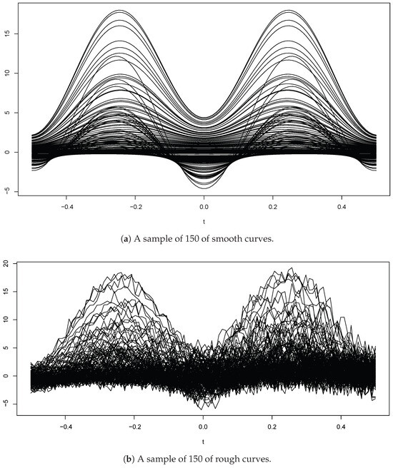
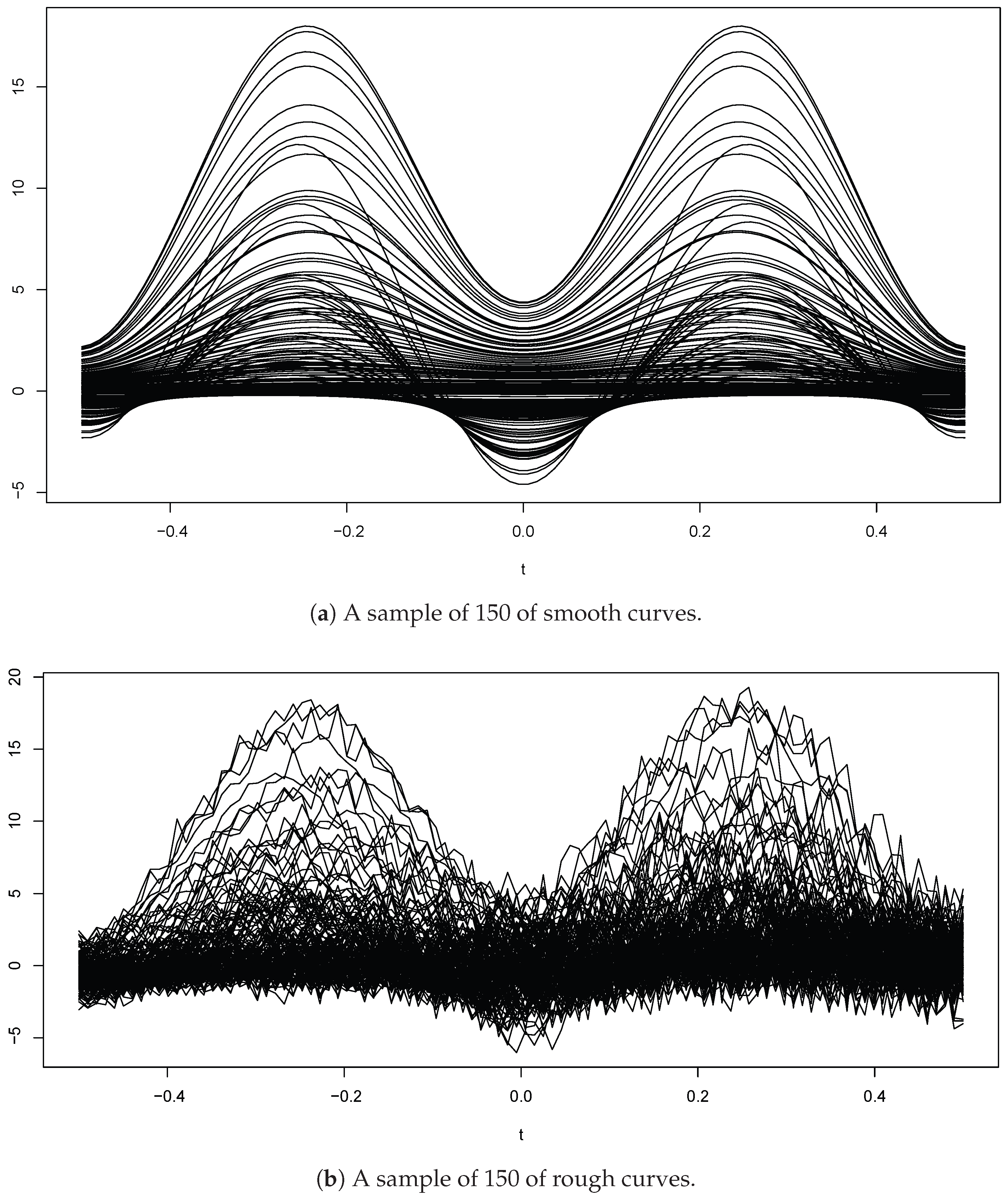
where $b_i$ is generated from $N(0,1)$ distribution and ${\eta }_i\left(t\right)$ is drown from $N(t,1+t)$ distribution. The curves are then discretized over a grid of points given by 100 equispaced measurements in $(0,1)$. A visual comparison of the two functional samples is provided in Figure 1.

Figure 1. A sample of 150 curves: smooth and roughy curves.

We model the scalar response S using the following non-parametric regression

$$S_i=3{\int }_{-0.5}^{0.5}{\displaystyle \frac{dt}{1+T_i^2\left(t\right)}}+{ϵ}_i\mathrm{for}i=1,\dots ,n,$$

(6)

where the errors $\left({ϵ}_i\right)$ are assumed to be independent of $\left(T_i\right)$. For the simulation study, we consider four error types of white noise generated from a normal mixture distribution, as follows:

$$\left\{\begin{array}{cc}\mathrm{S}\mathrm{t}\mathrm{a}\mathrm{n}\mathrm{d}\mathrm{a}\mathrm{r}\mathrm{d} \mathrm{n}\mathrm{o}\mathrm{r}\mathrm{m}\mathrm{a}\mathrm{l} \mathrm{d}\mathrm{i}\mathrm{s}\mathrm{t}\mathrm{r}\mathrm{i}\mathrm{b}\mathrm{u}\mathrm{t}\mathrm{i}\mathrm{o}\mathrm{n} (\mathrm{S}.\mathrm{N}.\mathrm{D}.)& N(0,1)\\ \mathrm{S}\mathrm{k}\mathrm{e}\mathrm{w}\mathrm{e}\mathrm{d} \mathrm{u}\mathrm{n}\mathrm{i}\mathrm{m}\mathrm{o}\mathrm{d}\mathrm{a}\mathrm{l} \mathrm{d}\mathrm{i}\mathrm{s}\mathrm{t}\mathrm{r}\mathrm{i}\mathrm{b}\mathrm{u}\mathrm{t}\mathrm{i}\mathrm{o}\mathrm{n} (\mathrm{S}.\mathrm{U}.\mathrm{D}.)& {\displaystyle \frac{1}{5}}N(0,1)+{\displaystyle \frac{1}{5}}N({\displaystyle \frac{1}{2}},{\displaystyle \frac{4}{9}})+{\displaystyle \frac{3}{5}}N({\displaystyle \frac{13}{12}},{\displaystyle \frac{25}{81}})\\ \mathrm{S}\mathrm{k}\mathrm{e}\mathrm{w}\mathrm{e}\mathrm{d} \mathrm{b}\mathrm{i}\mathrm{m}\mathrm{o}\mathrm{d}\mathrm{a}\mathrm{l} \mathrm{d}\mathrm{i}\mathrm{s}\mathrm{t}\mathrm{r}\mathrm{i}\mathrm{b}\mathrm{u}\mathrm{t}\mathrm{i}\mathrm{o}\mathrm{n} (\mathrm{C}.\mathrm{B}.\mathrm{D}.)& {\displaystyle \frac{3}{4}}N(0,1)+{\displaystyle \frac{1}{4}}N({\displaystyle \frac{3}{2}},{\displaystyle \frac{1}{9}})\\ \mathrm{C}\mathrm{l}\mathrm{a}\mathrm{w} \mathrm{d}\mathrm{i}\mathrm{s}\mathrm{t}\mathrm{r}\mathrm{i}\mathrm{b}\mathrm{u}\mathrm{t}\mathrm{i}\mathrm{o}\mathrm{n} (\mathrm{C}.\mathrm{D}.)& {\displaystyle \frac{1}{2}}N(0,1)+\sum _{i=1}^4{\displaystyle \frac{1}{10}}N({\displaystyle \frac{i}{2}}-1,{\displaystyle \frac{1}{100}})\end{array}\right.$$

(7)

Further details on normal mixture distributions can be found in [20]. Now, in order to compare the LOOCV to the Bootstrap selector, we optimize both rules over $\mathcal{M}$; the set of m ensures that the ball, centered at $\mathcal{T}$ with radius m, contains exactly k neighbors of $\mathcal{T}$. Specifically, the number k is selected from the subset $\{5,15,25,\dots ,75\}$. Observe that the Bootstrap selector requires a pilot bandwidth $m_0$ which is chosen using the R- routine h.default from the R-package 4.3 fda.usc. The two selection procedures performance are tested by comparing their averaged absolute errors ASE, where

$${\displaystyle \mathrm{ASE}=\frac{1}{150}\sum _{i=1}^{150}\left|S_i-\widehat{RER}\left(T_i\right)\right|.}$$

The model performance also depends critically on using a metric N. To highlight the easy of implementation of the RMT-based metric discussed in Section 4.3, we illustrate the impact of metric choice on accuracy by comparing the efficiency of the RMT-based metric against standard alternatives, such as the spline-based metric and the PCA metric. The first one is used for the smooth curves and is defined by derivatives,

$$N(\mathcal{T},{\mathcal{T}}^{\prime })={\left({\int }_0^1{({\mathcal{T}}^{\left(i\right)}\left(t\right)-{\mathcal{T}}^{\prime \left(i\right)}\left(t\right))}^{2}dt\right)}^{1/2},$$

where ${\mathcal{T}}^{\left(i\right)}$ denotes the ith derivative of the curve $\mathcal{T}$. Meanwhile, for the rough curves we compare the PCA semi-metric associated with the q-greatest eigenvalues. Although it is evident that LARE regression offers clear advantages over traditional LAD regression by measuring deviations relative to the magnitude of the response variable, we also illustrate this advantage by quantifying these gains through our empirical analysis. While the simulation study investigated numerous values of i, q, and n, we report here only the results for $i=2$, $q=1$, and $n=150,300$, for brevity. A quadratic kernel on $(0,1)$ was used for this empirical analysis. Table 1 and Table 2 summarize the obtained ASE results for different scenarios.

Table 1. ASE results for $n=150$. Comparison of smooth and rough curves under different regressions, metrics, distributions, and selector methods (LOOCV and Bootstrap).

Curves	Regression	Metric	Distribution	LOOCV	Bootstrap
Smooth curves	LARE regression	spline metric	S.N.D.	0.83	0.97
			S.U.D.	0.98	1.23
			S.B.D.	1.12	1.37
			C.D.	1.18	1.23
		RMT metric	S.N.D.	0.71	0.83
			S.U.D.	0.84	1.07
			S.B.D.	1.04	1.13
			C.D.	1.09	1.11
	LAD regression	spline metric	S.N.D.	1.12	1.33
			S.U.D.	1.21	1.44
			S.B.D.	1.49	1.52
			C.D.	1.73	1.91
		RMT metric	S.N.D.	0.93	1.17
			S.U.D.	1.12	1.21
			S.B.D.	1.36	1.41
			C.D.	1.61	1.76
Rough curves	LARE regression	PCA metric	S.N.D.	1.17	1.84
			S.U.D.	1.26	1.74
			S.B.D.	1.29	2.18
			C.D.	1.52	1.57
		RMT metric	S.N.D.	1.02	1.71
			S.U.D.	1.18	1.49
			S.B.D.	1.17	1.95
			C.D.	1.41	1.42
	LAD regression	PCA metric	S.N.D.	1.37	1.96
			S.U.D.	1.49	2.09
			S.B.D.	1.89	2.29
			C.D.	1.88	1.90
		RMT metric	S.N.D.	1.25	1.84
			S.U.D.	1.31	1.81
			S.B.D.	1.72	2.02
			C.D.	1.72	1.85

Table 2. ASE results for $n=300$. Comparison of smooth and rough curves under different regressions, metrics, distributions, and selector methods (LOOCV and Bootstrap).

Curves	Regression	Metric	Distribution	LOOCV	Bootstrap
Smooth curves	LARE regression	spline metric	S.N.D.	0.81	0.94
			S.U.D.	0.95	1.22
			S.B.D.	1.08	1.31
			C.D.	1.14	1.19
		RMT metric	S.N.D.	0.68	0.78
			S.U.D.	0.80	1.02
			S.B.D.	0.95	1.09
			C.D.	1.02	1.07
	LAD regression	spline metric	S.N.D.	1.10	1.31
			S.U.D.	1.16	1.40
			S.B.D.	1.46	1.48
			C.D.	1.67	1.86
		RMT metric	S.N.D.	0.91	1.14
			S.U.D.	1.06	1.18
			S.B.D.	1.31	1.38
			C.D.	1.58	1.74
Rough curves	LARE regression	PCA metric	S.N.D.	1.15	1.81
			S.U.D.	1.22	1.71
			S.B.D.	1.21	2.11
			C.D.	1.42	1.49
		RMT metric	S.N.D.	0.97	1.68
			S.U.D.	1.12	1.43
			S.B.D.	1.13	1.85
			C.D.	1.39	1.33
	LAD regression	PCA metric	S.N.D.	1.28	1.83
			S.U.D.	1.36	1.95
			S.B.D.	1.75	2.17
			C.D.	1.73	1.83
		RMT metric	S.N.D.	1.14	1.71
			S.U.D.	1.19	1.79
			S.B.D.	1.64	1.93
			C.D.	1.63	1.72

We observe that the LOOCV strategy yields superior results compared to the Bootstrap method. This advantage is pronounced in the case of Skewed Bimodal Distributions (S.B.D.), whereas, for Contaminated Distributions (C.D.), the two methods perform nearly equivalently. Furthermore, both bandwidth selectors demonstrate relatively strong efficiency across the tested scenarios. Although estimation accuracy generally improves as the sample size n increases, the choice of metric has a substantial impact on estimation quality. Unsurprisingly, the RMT metric consistently outperforms the standard metric. Moreover, the superiority of LARE regression over LAD regression is also evident. This advantage arises from the proportional treatment of deviations in LARE regression, which allows both small and large responses to be appropriately weighted. In contrast, LAD regression assigns equal weight to all deviations, a property that may lead to biased estimates when the response variable exhibits considerable variation in scale.

In the second part of this illustration, we examine the robustness of the proposed estimator by comparing it to the LSER regression defined by

$$\widetilde{RER}={\displaystyle \frac{{\sum }_{i=1}^n{S}_i^{-1}M\left(m^{-1}N(\mathcal{T},T_i)\right)|}{{\sum }_{i=1}^{n}M\left(m^{-1}N(\mathcal{T},T_i)\right)S_i^{-2}}}.$$

It is important to note that robustness can be assessed through various metrics, including the influence function, gross-error sensitivity, breakdown point, local shift sensitivity or bias/variance under contamination, among others (see [21,22,23] for a comprehensive overview). While some of these metrics are challenging to apply in the context of functional statistics, they all share the common goal of evaluating the stability of a statistical method and quantifying its sensitivity to deviations from model assumptions. In this experiment, we assess robustness by analyzing the variance under the contaminated data-generating process. Specifically, we construct a contamination model by taking it as a white noise, where

$${\epsilon }_i=t{\epsilon }_{1_i}+(1-t){\epsilon }_{2_i},t\in (0,1),i=1,2,$$

where ${\epsilon }_{1_i}$ is generated from S.N.D and ${\epsilon }_{2_i}$ is drown from C.D. Under this contamination, the empirical variance is defined by

$$V\left(t\right)=Var{(\widehat{RER}\left(T_i\right))}_{i=1}^n.$$

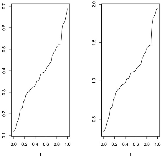
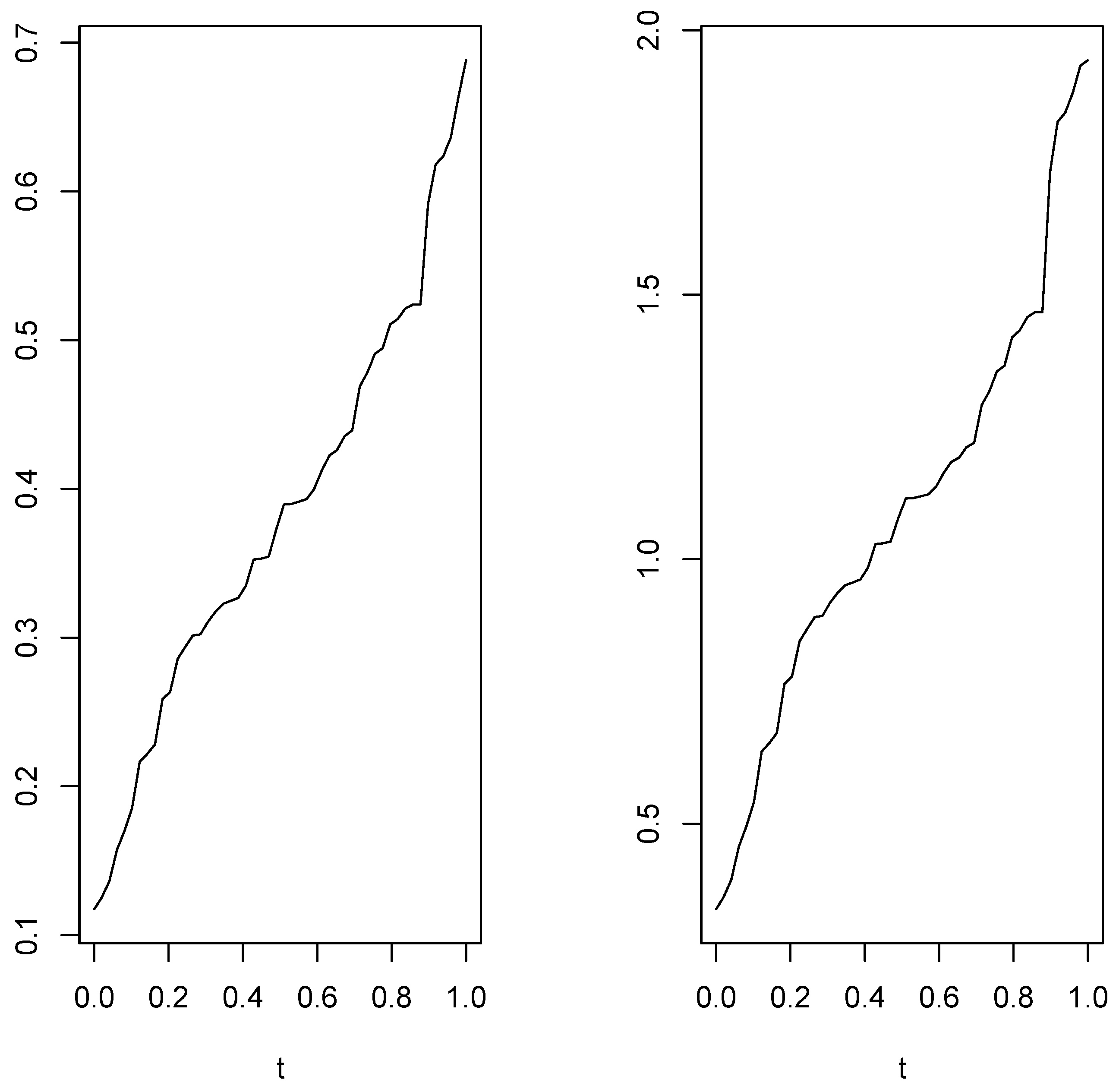
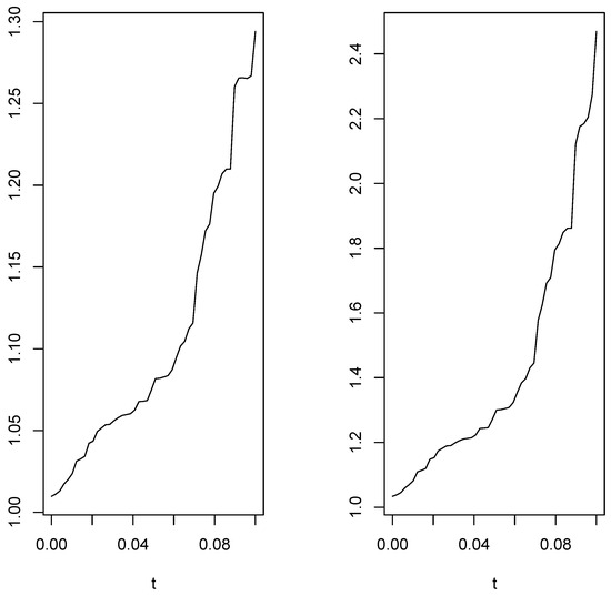
In Figure 2 and Figure 3, we plot the function $V\left(t\right)$ for both estimators using both cases (smooth and rough case).

Figure 2. The variability of the function $V\left(t\right)$ over 50 points in $(0,1)$ in the smooth case: (Left) LARE regression; (Right) LSRE regression.

Figure 3. The variability of the function $V\left(t\right)$ over 50 points in $(0,1)$ in the rough case. (Left) LARE regression, (Right) LSRE regression.

It is not surprising that Figure 2 and Figure 3 confirm the robustness of $\widehat{RER}$ compared to $\widetilde{RER}$. It shows that the function $V\left(t\right)$ of $\widehat{RER}$ has a small variation compared to the variation in $\widetilde{RER}$. This conclusion is confirmed by computing the range of $V\left(t\right)$, defined as

$$RG=maxV\left(t\right)-minV\left(t\right),$$

which serves as a measure of the function’s variability. This benchmark is computed over 50 discretized points in the interval (0, 1). Specifically, in the smooth case, we obtained $0.6$ for the LARE regression compared to $1.9$ for the LSRE regression. The same statement for the rough case was observed, and RG = 0.3 for the LARE regressions against $RG=1.45$ for the LSRE regression case.

5.2. Real Data Application

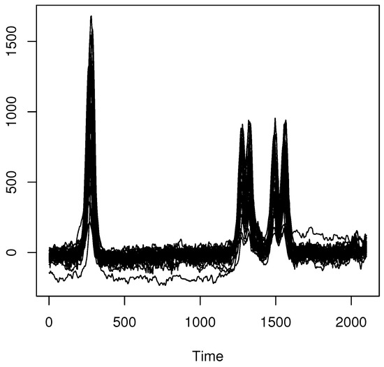
This section presents a predictive analysis using the LARE model. Specifically, we conduct a comparative study of several regression predictors. More precisely, we focus in this empirical analysis on the prediction of the sulfone content in onion diets using near-infrared (NIR) spectral curves. Sulfones are organic compounds highly beneficial to human health. Their biomedical significance is well documented in the literature, with studies indicating efficacy in treating conditions such as mucous-membrane inflammation and gastrointestinal disorders. Furthermore, research has highlighted their potential to suppress tumor initiation (see [24]). Our objective is to use the NIR spectrometry to quantify the relationship between onion consumption in a rodent model and subsequent sulfone levels in urine. The functional NIR data utilized in this analysis are available on the website http://www.models.life.ku.dk (accessed on 20 October 2025). It is well known that the nonparametric functional statistics provide a powerful framework for analyzing near-infrared (NIR) spectroscopy data. Typically, treating NIR spectra as functional observations allows for exploration of the smooth variations across wavelengths, and improvements in the accuracy of prediction. Thus, the functional treatment of the NIR data is a more robust tool for extracting meaningful information. The sample preparation involved a two-step chemical process: initial spectrometry processing followed by spectral acquisition in the wavelength region from 9.6 to 0.3 ppm. The resulting dataset comprises 32 observations, which were recolored with sufficient replication. The spectral curves for these observations are plotted in Figure 4. Further details on this dataset are available in [24].

Figure 4. The spectral curves of the NIR data comprising 32 observations.

For the prediction task, we compare the performance of three regression estimators:

$$\begin{array}{cc}\hfill {\displaystyle \widehat{RER}\left(\mathcal{T}\right)=arg\underset{s}{min}\frac{{\sum }_{i=1}^{n}M\left(m^{-1}N(\mathcal{T},T_i)\right)\left|\frac{S_i-s}{S_i}\right|}{{\sum }_{i=1}^{n}M\left(m^{-1}N(\mathcal{T},T_i)\right)}}& (\mathrm{LARE}\mathrm{Regression}),\hfill \\ \hfill \widetilde{RER}\left(\mathcal{T}\right)={\displaystyle \frac{{\sum }_{i=1}^n{S}_i^{-1}M\left(m^{-1}N(\mathcal{T},T_i)\right)|}{{\sum }_{i=1}^{n}M\left(m^{-1}N(\mathcal{T},T_i)\right)S_i^{-2}}}& (\mathrm{LSRE}\mathrm{Regression}),\hfill \\ \hfill \overline{RE}\left(\mathcal{T}\right)={\displaystyle \frac{{\sum }_{i=1}^n{S}_{i}M\left(m^{-1}N(\mathcal{T},T_i)\right)|}{{\sum }_{i=1}^{n}M\left(m^{-1}N(\mathcal{T},T_i)\right)}}& (\mathrm{NW}\mathrm{Regression}).\hfill \end{array}$$

To ensure a fair comparison, common computational strategies were employed for the three estimators. This includes the use of the RMT metric, an identical kernel function M and the application of the rule specified in Equation (5) for selecting the bandwidth parameter for the three methods.

To evaluate the robustness of these estimators, we introduced a contamination by multiplying a subset of observations by a factor of 10. The impact of this contamination was assessed by controlling the variation in the Mean Absolute Error (MAE). Specifically, for a given contamination proportion $t\in [0,1]$, we multiplied $\left[tn\right]$ observations (where $[.]$ denotes the integer part) and computed the variability of the prediction error function using

$$\mathrm{AME}\left(t\right)={\displaystyle \frac{1}{35}}\sum _{k=1}^{35}(S_k-\dot{Pred}\left(T_k\right)),$$

where $\dot{Pred}$ denotes one of the three compared estimators. The resulting prediction errors are displayed in Figure 5.

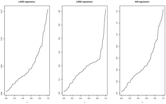
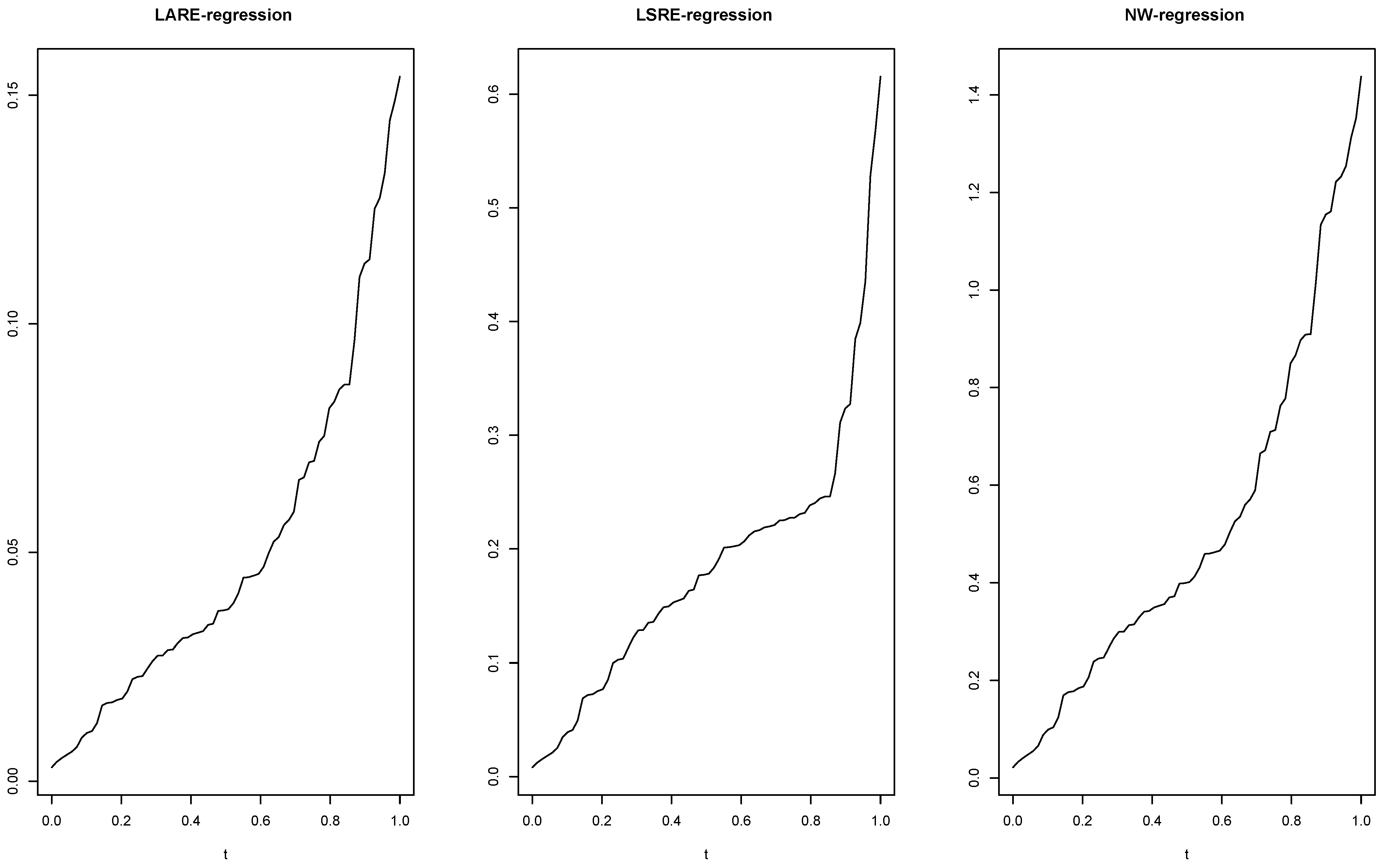
Figure 5. Comparison of prediction errors across the three regression estimators under increasing data contamination.

The results indicate that, while all three predictors have satisfactory performance under uncontaminated conditions ($t=0$), the LARE approaches demonstrate a significant advantage. This advantage is particularly evident in the stability of the LARE estimator ($\widehat{RER}$), which exhibits lower variability in its MAE under contamination. The superior stability of the LARE method is quantitatively confirmed by examining the range of its error function. The range of the LARE regression was observed to be between $0.02$ and $0.15$, compared to a range of $[0.02,0.6]$ for the LSRE regression and $[0.05,1.4]$ for the standard nonparametric regression. This empirical finding aligns with the theoretical expectation that estimators based on the absolute relative error (LARE) are more robust than those based on the squared error (LSRE), due to the reduced influence of large residuals. It should be noted that the accuracy of the estimator is affected by the sample size of the data. However, since our main purpose is to investigate the robustness of the proposed estimator, the effect of the sample size is omitted. One reason is that the robustness is assessed in terms of stability rather than accuracy. The robustness property is highlighted by the variability of the estimation error, which shows that the LARE estimator is more stable and less sensitive to added outliers.

6. Conclusions and Prospects

This work introduces a robust framework for functional regression estimation by employing the least absolute relative error loss function. We construct a novel estimator and establish its asymptotic properties, specifically, proving its complete consistency. The functional structure is modeled using the small ball probability function that relates the topological structure of the probability measure of the functional explanatory variable. Furthermore, the employment of the LARE rule significantly increases the robustness of the model. The derived asymptotic results are obtained under general assumptions, ensuring their applicability to a broad class of functional data and continuous-time processes. Empirical analyses illustrate the straightforward implementation of our estimator. We have shown that the estimator can be applied easily, and various technical approaches are available to select the principal parameters involved. Moreover, the computational results highlight the superiority of the LSRE regression in terms of both robustness and predictive accuracy compared with alternative methods. This contribution opens several promising questions for future research. A natural extension would be to develop a local linear version of this robust modal regression estimator. It is well-known that the local linear modeling can improve the asymptotic convergence rate by reducing boundary bias. Establishing the asymptotic normality of the proposed robust estimator is another critical open question, as it is a prerequisite for constructing confidence intervals and conducting hypothesis tests. Other important directions include exploring linear or partially linear formulations of this regression. A particularly challenging but impactful extension would be to adapt these methods to more complex data structures, such as censored data or functional time series. Addressing such complexities will require the development of new mathematical tools and theoretical advances that go beyond the scope of the present study.

References

- Ferraty, F.; Vieu, P. The functional nonparametric model and application to spectrometric data. Comput. Stat. 2002, 17, 545–564. [Google Scholar] [CrossRef] [Scilit]
- Dabo-Niang, S.; Rhomari, N. Estimation non paramétrique de la régression avec variable explicative dans un espace métrique. Comptes Rendus MathéMatique 2003, 336, 75–80. [Google Scholar] [CrossRef] [Scilit]
- Delsol, L. Régression non-paramétrique fonctionnelle: Expressions asymptotiques des moments. In Annales de l’ISUP; LSTA: Paris, France, 2007; Volume 51, pp. 43–67. [Google Scholar]
- Masry, E. Nonparametric regression estimation for dependent functional data: Asymptotic normality. Stoch. Process. Their Appl. 2005, 115, 155–177. [Google Scholar] [CrossRef] [Scilit]
- Barrientos-Marin, J.; Ferraty, F.; Vieu, P. Locally modelled regression and functional data. J. Nonparametr. Stat. 2010, 22, 617–632. [Google Scholar] [CrossRef] [Scilit]
- Narula, S.C.; Wellington, J.F. Prediction, linear regression and the minimum sum of relative errors. Technometrics 1977, 19, 185–190. [Google Scholar] [CrossRef]
- Chatfield, C. The joys of consulting. Significance 2007, 4, 33–36. [Google Scholar] [CrossRef] [Scilit]
- Chen, K.; Guo, S.; Lin, Y.; Ying, Z. Least absolute relative error estimation. J. Am. Stat. Assoc. 2010, 105, 1104–1112. [Google Scholar] [CrossRef] [Scilit] [PubMed]
- Yang, Y.; Ye, F. General relative error criterion and M-estimation. Front. Math. China 2013, 8, 695–715. [Google Scholar] [CrossRef] [Scilit]
- Jones, M.C.; Park, H.; Shin, K.I.; Vines, S.K.; Jeong, S.O. Relative error prediction via kernel regression smoothers. J. Stat. Plan. Inference 2008, 138, 2887–2898. [Google Scholar] [CrossRef] [Scilit]
- Attouch, M.; Laksaci, A.; Messabihi, N. Nonparametric relative error regression for spatial random variables. Stat. Pap. 2017, 58, 987–1008. [Google Scholar] [CrossRef] [Scilit]
- Demongeot, J.; Hamie, A.; Laksaci, A.; Rachdi, M. Relative-error prediction in nonparametric functional statistics: Theory and practice. J. Multivar. Anal. 2016, 146, 261–268. [Google Scholar] [CrossRef] [Scilit]
- Altendji, B.; Demongeot, J.; Laksaci, A.; Rachdi, M. Functional data analysis: Estimation of the relative error in functional regression under random left-truncation model. J. Nonparametr. Stat. 2018, 30, 472–490. [Google Scholar] [CrossRef] [Scilit]
- Benzamouche, S.; Ould Saïd, E.; Sadki, O. Nonparametric estimation of the relative error regression for twice censored and dependent data. Commun. Stat.-Theory Methods 2025, 54, 1492–1525. [Google Scholar] [CrossRef] [Scilit]
- Xia, X.; Ming, H.; Li, J. Relative error model average for multiplicative models. Stat. Comput. 2026, 36, 18. [Google Scholar] [CrossRef] [Scilit]
- Wang, J.L.; Chiou, J.M.; Müller, H.G. Functional data analysis. Annu. Rev. Stat. Its Appl. 2016, 3, 257–295. [Google Scholar] [CrossRef] [Scilit]
- Aneiros, G.; Bongiorno, E.G.; Goia, A.; Hušková, M. (Eds.) New Trends in Functional Statistics and Related Fields; Springer Nature: New York, NY, USA, 2025. [Google Scholar]
- Ndiaye, M.; Dabo-Niang, S.; Ngom, P.; Thiam, N.; Brehmer, P.; El Vally, Y. Nonparametric prediction and supervised classification for spatial dependent functional data under fixed sampling design. In Nonlinear Analysis, Geometry and Applications: Proceedings of the Third NLAGA-BIRS Symposium, AIMS-Mbour, Senegal, 21–27 August 2023; Springer Nature: Cham, Switzerland, 2024; pp. 69–100. [Google Scholar]
- Ferraty, F.; Vieu, P. Nonparametric Functional Data Analysis: Theory and Practice; Springer: New York, NY, USA, 2006. [Google Scholar]
- Benaglia, T.; Chauveau, D.; Hunter, D.R.; Young, D.S. Mixtools: An R package for analyzing mixture models. J. Stat. Softw. 2010, 32, 1–29. [Google Scholar]
- Huber, P.J.; Ronchetti, E.M. Robust Statistics, 2nd ed.; John Wiley & Sons: Hoboken, NJ, USA, 2009. [Google Scholar]
- Hampel, F.R. A general qualitative definition of robustness. Ann. Math. Stat. 1971, 42, 1887–1896. [Google Scholar] [CrossRef] [Scilit]
- Maronna, R.A.; Martin, R.D.; Yohai, V.J.; Salibian-Barrera, M. Robust Statistics: Theory and Methods (with R); John Wiley & Sons: Hoboken, NJ, USA, 2019. [Google Scholar]
- Winning, H.; Roldán-Marín, E.; Dragsted, L.O.; Viereck, N.; Poulsen, M.; Sánchez-Moreno, C.; Cano, M.P.; Engelsen, S.B. An exploratory NMR nutri-metabonomic investigation reveals dimethyl sulfone as a dietary biomarker for onion intake. Analyst 2009, 134, 2344–2351. [Google Scholar] [CrossRef] [Scilit] [PubMed]
- Koenker, R.; Zhao, Q. Conditional quantile estimation and inference for ARCH models. Econom. Theory 1996, 12, 793–813. [Google Scholar] [CrossRef] [Scilit]
Disclaimer/Publisher’s Note: The statements, opinions and data contained in all publications are solely those of the individual author(s) and contributor(s) and not of MDPI and/or the editor(s). MDPI and/or the editor(s) disclaim responsibility for any injury to people or property resulting from any ideas, methods, instructions or products referred to in the content. |
© 2026 by the authors. Licensee MDPI, Basel, Switzerland. This article is an open access article distributed under the terms and conditions of the Creative Commons Attribution (CC BY) license.