Optimal Feedback Policy for the Tracking Control of Markovian Jump Boolean Control Networks over a Finite Horizon

Abstract

This paper aims to find optimal feedback policies for the tracking control of Markovian jump Boolean control networks (MJBCNs) over a finite horizon. The tracking objective is a predetermined time-varying trajectory with a finite length. To minimize the expected total tracking error between the output trajectory of MJBCN and the reference trajectory, an algorithm is proposed to determine the optimal policy for the system. Furthermore, considering the penalty for control input changes, a new objective function is obtained by weighted summing the total tracking error with the total variation of control input. Certain optimal policies sre designed using an algorithm to minimize the expectation of the new objective function. Finally, the methodology is applied to two simplified biological models to demonstrate its effectiveness.

1. Introduction

Boolean networks (BNs) were first put forward by Kauffman as a kind of model for genetic regulatory networks (GRNs) [1]. When simulating a GRN with a BN, each node of the BN represents a gene, whose state is quantified as 1 or 0, and the genes’ mutual regulatory interactions are characterized by logical functions. Moreover, sometimes, there are external drug interventions in GRNs, which can be interpreted as control inputs in BNs. BNs with control input nodes are termed Boolean control networks (BCNs). There was no unified tool for studying BNs until semi-tensor product (STP) was proposed [2], which has greatly facilitated research on many related problems regarding BNs, including stability and stabilization [3,4,5], controllability and observability [6,7,8], state estimation [9,10,11,12], state compression [13], and the output tracking control (OTC) problem [14,15,16,17]. In addition, STP has also been widely adopted in other areas like nonlinear shift registers [18] and fuzzy relational inequalities [19].

As we know, there is usually randomness in gene expression. Consequently, Shmulevich et al. proposed probabilistic Boolean networks (PBNs) to characterize the uncertainty in GRNs [20,21]. A PBN has several realizations, and each realization is selected according to a probability distribution for each time. Similarly, probabilistic Boolean control networks (PBCNs) are derived from PBNs by incorporating control inputs into networks. In addition, a Markov chain was shown to emulate the dynamic of a small GRN well [22]. Furthermore, Markovian jump Boolean control networks (MJBCNs) form another category of stochastic extensions to BNs. As stated in [23], PBCNs can be regarded as a special kind of MJBCNs. In an MJBCN, mode transitions are governed by a Markov chain. Recently, some results on MJBCNs have been obtained, such as controllability [23] and stabilization [24,25].

The significance of OTC lies in its ability to design the control so that the system output closely follows a desired reference trajectory. This is valuable in various practical applications such as robotic manipulator control [26] and flight control [27]. By solving the OTC problem, systems can operate stably in dynamic environments, reduce errors, improve performance, and lower costs and energy consumption. In fields like disease treatment, it can also help precisely control drug concentrations and treatment processes, enhancing effectiveness and safety. The finite-time OTC of BCNs was first investigated by Li et al. [14,15]. Moreover, the finite-time OTC of PBCNs has been studied in [28]. In addition, the asymptotic OTC of PBCNs has been addressed by Chen et al. [29]. In these studies, the tracking objective is a constant state or a reference system.

As stated in [30], a useful method to improve the efficiency of bioreactors is forcing the states of microalgas to follow a predetermined reference trajectory. Motivated by this, Zhang et al. [16] investigated the optimal (i.e., minimum error) OTC of BCNs over a finite time horizon, where the tracking objective is a predefined finite-length trajectory. Moreover, in practice, it is difficult to make substantial changes to the control inputs in a short period, or it may require increased costs. For example, in disease treatment, the concentration of a drug in the body typically decreases gradually rather than instantaneously. Thus, the penalty for the control input changes was taken into account in [16]. After that, the OTC problems of PBCNs and MJBCNs with respect to a predefined reference trajectory were studied in [31,32,33], respectively. However, there was no feedback policy provided for all of the initial states in [33]; moreover, a penalty for control input changes was not considered in [31,32,33].

In this article, we study the finite horizon OTC of MJBCNs with respect to a predefined reference trajectory with a finite length.

• The OTC problem is reformulated as an optimal control problem, and then an optimal policy is obtained to minimize the expected total tracking error.
• A new objective function is constructed by performing a weighted sum of the total tracking error and the total variation of the control input. An optimal policy is given to minimize the expected objective function value.
• The optimal feedback policies obtained in this paper apply to all initial states. As shown in the examples, the design of policies is based on the specific weightings given to the two objectives (i.e., reducing tracking errors and decreasing input variations).

The rest of the paper is organized as follows. Section 2 introduces some preliminaries. In Section 3, the main results on the optimal finite horizon OTC of MJBCNs are obtained. Two examples are given in Section 4 to demonstrate the results. Finally, concluding remarks are provided in Section 5.

2. Preliminaries

The basic symbols are given in Table 1. Due to STP being a generalization of ordinary matrix multiplication [2], in the sequel, we omit symbol ⋉ as long as there is no ambiguity.

Table 1. Notations.

Notations	Definitions
$\mathbb{N}$	Set of natural numbers
$\mathcal{D}$, ${\mathcal{D}}^n$	$\{0,1\}$, $\underset{\underset{n}{︸}}{\mathcal{D}\times \mathcal{D}\times \cdots \times \mathcal{D}}$
$I_n$	n-dimensional identity matrix
${\delta }_n^i$	i-th column of $I_n$
${\mathsf{\Delta }}_n$	Set of columns of $I_n$; $\mathsf{\Delta }:={\mathsf{\Delta }}_2$
$\mathbf{v}\left(X\right)$	Vector form of $X\in \mathcal{D}$, i.e., $\mathbf{v}\left(X\right)={\delta }_2^{2-X}\in \mathsf{\Delta }$
${\left[A\right]}_{ij}$	$(i,j)$-th entry of the matrix A
${\mathrm{Col}}_i\left(A\right)$	i-th column of the matrix A
${\left[v\right]}_i$	i-th entry of the vector v
$[n:m]$	Set of integers $\{n,n+1,\dots ,m\}$
${\delta }_n[i_1{i}_2\cdots i_m]$	The logical matrix of which k-column is ${\delta }_n^{i_k}$
${\mathbb{R}}_{n\times m}$	Set of $n\times m$ real matrices
${\mathcal{L}}_{n\times m}$	Set of $n\times m$ logical matrices
⊗	Kronecker product
⋉	Semi-tensor product [2]
*	Khatri-Rao product [34]
${⋉}_{i=1}^n{x}_i$	Short for $x_1⋉x_2⋉\cdots ⋉x_n$
${\mathbf{1}}_n$, ${\mathbf{0}}_n$, ${\mathbf{\infty }}_n$	${\left[\underset{\underset{n}{︸}}{11\cdots 1}\right]}^{⊺}$,  ${\left[\underset{\underset{n}{︸}}{00\cdots 0}\right]}^{⊺}$ ${\left[\underset{\underset{n}{︸}}{\infty \infty \cdots \infty }\right]}^{⊺}$

MJBCN is presented as follows:

$$\left\{\begin{array}{c}{X}_i(t+1)=f_i^{\sigma \left(t\right)}(X\left(t\right),U\left(t\right)),i=1,\dots ,n,\hfill \\ Y_j\left(t\right)=h_j\left(X\left(t\right)\right),j=1,\dots ,q,\hfill \end{array}\right.$$

(1)

where $X\left(t\right)=(X_1\left(t\right),X_2\left(t\right),\dots ,X_n\left(t\right))\in {\mathcal{D}}^n$ is the state vector, $U\left(t\right)=(U_1\left(t\right),U_2\left(t\right),\dots ,$$U_m\left(t\right))\in {\mathcal{D}}^m$ is the control input vector, $Y\left(t\right)=(Y_1\left(t\right),Y_2\left(t\right),\dots ,Y_q\left(t\right))\in {\mathcal{D}}^q$ is the output vector, and $\sigma \left(t\right)\in [1:s]$ is a Markov switching signal with a transition probability matrix (TPM) $P={\left(p_{ij}\right)}_{s\times s}$, that is, $\mathbf{Pr}\{\sigma (t+1)=j\mid \sigma \left(t\right)=i\}=p_{ij},\forall i,j\in [1:s]$. In addition, all $f_i^k,k\in [1:s],i\in [1:n]$ and $h_j,j\in [1:q]$ are logical mappings.

Let $x\left(t\right)={⋉}_{i=1}^n\mathbf{v}\left(X_i\left(t\right)\right)\in {\mathsf{\Delta }}_{2^n}$, $y\left(t\right)={⋉}_{j=1}^q\mathbf{v}\left(Y_j\left(t\right)\right)\in {\mathsf{\Delta }}_{2^q}$ and $u\left(t\right)={⋉}_{k=1}^m\mathbf{v}\left(U_k\left(t\right)\right)\in {\mathsf{\Delta }}_{2^m}$. Then MJBCN (1) can be converted into [24]:

$$\left\{\begin{array}{c}x(t+1)=F_{\sigma \left(t\right)}u\left(t\right)x\left(t\right),\hfill \\ y\left(t\right)=Hx\left(t\right),\hfill \end{array}\right.$$

(2)

where $F_i\in {\mathcal{L}}_{2^n\times 2^{n+m}}$, $i\in [1:s]$ and $H\in {\mathcal{L}}_{2^q\times 2^n}$.

Assumption 1

([35]). $x(t+1)$ and $\sigma (t+1)$ are conditionally independent of $x\left(t\right),\sigma \left(t\right),u\left(t\right)$ for all $t>0$.

Let $N=s{2}^n$, $M=2^m$, and $\tilde{F}=[F_1{F}_2\cdots F_s]\in {\mathcal{L}}_{2^n\times NM}$. Introduce instrumental variables $\omega \left(t\right)={\delta }_s^{\sigma \left(t\right)}\in {\mathsf{\Delta }}_s$ and $z\left(t\right)=\omega \left(t\right)x\left(t\right)\in {\mathsf{\Delta }}_N$. Define a matrix

$$\widehat{F}=\left({\mathbf{1}}_M^{⊺}\otimes P^{⊺}\otimes {\mathbf{1}}_{2^n}^{⊺}\right)\ast \left(\tilde{F}{W}_{[M,s]}\right).$$

(3)

where $W_{[M,s]}=[I_s\otimes {\delta }_M^1{I}_s\otimes {\delta }_M^2\cdots I_s\otimes {\delta }_M^M]$ is called the swap matrix [2]. Split matrix $\widehat{F}$ into M blocks of the same size: $\widehat{F}=\left[{\overline{F}}_1{\overline{F}}_2\cdots {\overline{F}}_{2^m}\right]$.

Proposition 1.

For any ${\delta }_N^i,{\delta }_N^j\in {\mathsf{\Delta }}_N$ and ${\delta }_M^k\in {\mathsf{\Delta }}_M$,

$$\mathbf{Pr}\{z(t+1)={\delta }_N^i\mid z\left(t\right)={\delta }_N^j,u\left(t\right)={\delta }_M^k\}={\left[{\overline{F}}_k\right]}_{ij}.$$

Proof. 

Suppose ${\delta }_N^i={\delta }_s^{{\gamma }_i}{\delta }_{2^n}^{{\xi }_i}$ and ${\delta }_N^j={\delta }_s^{{\gamma }_j}{\delta }_{2^n}^{{\xi }_j}$. Note that $x(t+1)=\tilde{F}\omega \left(t\right)u\left(t\right)x\left(t\right)=\tilde{F}{W}_{[M,s]}u\left(t\right)z\left(t\right)$, so

$$\mathbf{Pr}\{x(t+1)={\delta }_{2^n}^{{\xi }_i}\mid z\left(t\right)={\delta }_N^j,u\left(t\right)={\delta }_M^k\}={\left[\tilde{F}{W}_{[M,s]}{\delta }_M^k\right]}_{{\xi }_{i}j}.$$

Moreover, note that $\mathbf{Pr}\{\sigma (t+1)={\gamma }_i\mid \sigma \left(t\right)={\gamma }_j\}={\left[P^{⊺}\right]}_{{\gamma }_i{\gamma }_j}$, so

$$\mathbf{Pr}\{\sigma (t+1)={\gamma }_i\mid z\left(t\right)={\delta }_N^j,u\left(t\right)={\delta }_M^k\}={\left[P^{⊺}\right]}_{{\gamma }_i{\gamma }_j}={[P^{⊺}\otimes {\mathbf{1}}_{2^n}^{⊺}]}_{{\gamma }_{i}j}.$$

Therefore, under Assumption 1,

$$\begin{array}{cc}\hfill & \mathbf{Pr}\{z(t+1)={\delta }_N^i\mid z\left(t\right)={\delta }_N^j,u\left(t\right)={\delta }_M^k\}\hfill \\ \hfill =& \mathbf{Pr}\{\sigma (t+1)={\gamma }_i,x(t+1)={\delta }_{2^n}^{{\xi }_i}\mid z\left(t\right)={\delta }_N^j,u\left(t\right)={\delta }_M^k\}\hfill \\ \hfill =& \mathbf{Pr}\{\sigma (t+1)={\gamma }_i\mid \sigma \left(t\right)={\gamma }_j,x\left(t\right)={\delta }_{2^n}^{{\xi }_j},u\left(t\right)={\delta }_M^k\}\hfill \\ \hfill & \times \mathbf{Pr}\{x(t+1)={\delta }_{2^n}^{{\xi }_i}\mid z\left(t\right)={\delta }_N^j,u\left(t\right)={\delta }_M^k\}\hfill \\ \hfill =& {[P^{⊺}\otimes {\mathbf{1}}_{2^n}^{⊺}]}_{{\gamma }_{i}j}\times {\left[\tilde{F}{W}_{[M,s]}{\delta }_M^k\right]}_{{\xi }_{i}j}={\left[{\overline{F}}_k\right]}_{ij},\hfill \end{array}$$

That is, $\mathbf{Pr}\{z(t+1)={\delta }_N^i\mid z\left(t\right)={\delta }_N^j,u\left(t\right)={\delta }_M^k\}={\left[{\overline{F}}_k\right]}_{ij}$.    □

3. Main Results

3.1. Finite Horizon OTC of MJBCNs

A reference trajectory of length $T\in \mathbb{N}$ is given as follows:

$$y^r\left(1\right)={\delta }_{2^q}^{r_1},y^r\left(2\right)={\delta }_{2^q}^{r_2},\dots ,y^r\left(T\right)={\delta }_{2^q}^{r_T},$$

(4)

where $r_t\in [1:2^q]$, $t=1,\dots ,T$.

A policy is a sequence of mappings in the form of $\pi =\{{\varphi }_0,{\varphi }_1,\dots ,{\varphi }_{T-1}\}$, where ${\varphi }_t:{\mathsf{\Delta }}_N\to {\mathsf{\Delta }}_M$$\forall t\in [0:T-1]$. There is a $K_{{\varphi }_t}\in {\mathcal{L}}_{M\times N}$ for each ${\varphi }_t$ such that ${\varphi }_t\left(z\left(t\right)\right)=K_{{\varphi }_t}z\left(t\right)$. If policy $\pi$ is determined, we stipulate

$$u\left(t\right)=K_{{\varphi }_t}z\left(t\right),t\in [0:T-1].$$

(5)

Conversely, if the feedback control (5) is given, policy $\pi$ is also determined. $\mathsf{\Pi }$ represents the set of all policies.

Definition 1.

The reference trajectory (4) is considered exactly tracked by MJBCN (2) via policy π under the initial condition $z\left(0\right)=z_0\in {\mathsf{\Delta }}_N$ if

$$\mathbf{Pr}\{y\left(t\right)=y^r\left(t\right)\mid z\left(0\right)=z_0,\pi \}=1,\forall t\in [1:T].$$

If the reference output trajectory (4) can not be exactly tracked, we attempt to find a policy $\pi \in \mathsf{\Pi }$ that can minimize the expected total tracking error between the output trajectory of MJBCN (2) and the reference trajectory (4) from $t=1$ to $t=T$.

Given two output state vectors $Y^{\prime }=(Y_1^{\prime },Y_2^{\prime },\dots ,Y_q^{\prime })\in {\mathcal{D}}^q$ and $Y^{″}=(Y_1^{″},Y_2^{″},\dots ,Y_q^{″})\in {\mathcal{D}}^q$, let $y_1={⋉}_{i=1}^q\mathbf{v}\left(Y_i^{\prime }\right)\in {\mathsf{\Delta }}_{2^q}$ and $y_2={⋉}_{i=1}^q\mathbf{v}\left(Y_i^{″}\right)\in {\mathsf{\Delta }}_{2^q}$. The distance between $y_1$ and $y_2$ (or between $Y^{\prime }$ and $Y^{″}$) is given as follows [16]:

$$d(y_1,y_2)=\sum _{i=1}^q|Y_i^{\prime }-Y_i^{″}|.$$

(6)

For example, suppose $Y^{\prime }=(1,1,1)$ and $Y^{″}=(0,1,1)$. We can calculate $y_1={\delta }_8^1$ and $y_2={\delta }_8^5$. By (6), $d(y_1,y_2)=1$. Although $Y^{\prime }$ and $y_1$ (likewise $Y^{″}$ and $y_2$) uniquely determine each other, $d(y_1,y_2)$ cannot be intuitively observed from $y_1={\delta }_8^1$ and $y_2={\delta }_8^5$. In fact, the Euclidean distance $\parallel y_1-y_2\parallel$ of $y_1$ and $y_2$ is either 0 or $\sqrt{2}$, which cannot reflect the degree of difference between $Y^{\prime }$ and $Y^{″}$. The distance formula (6) represents the number of different components of $Y^{\prime }$ and $Y^{″}$. In comparison, the distance formula (6) is more in line with our requirements than the Euclidean distance.

The total tracking error between the output trajectory of MJBCN (2) and the reference trajectory (4) is expressed as

$$\begin{array}{c}\hfill e(z\left(0\right),y,y^r)=\sum _{t=1}^{T}d(y\left(t\right),y^r\left(t\right)).\end{array}$$

(7)

As the output state vectors of system (2) are finite in number, $\mathbb{E}\left\{e(z\left(0\right),y,y^r)\right\}=0$ means that MJBCN (2) exactly tracks the reference trajectory (4). We intend to find a policy to minimize $\mathbb{E}\left\{e(z\left(0\right),y,y^r)\right\}$ for all $z\left(0\right)\in {\mathsf{\Delta }}_N$.

Define weight factor vectors:

$$\begin{array}{cc}\hfill & C\left(T\right)=[d({\delta }_{2^q}^1,{\delta }_{2^q}^{r_T})d({\delta }_{2^q}^2,{\delta }_{2^q}^{r_T})\cdots d({\delta }_{2^q}^{2^q},{\delta }_{2^q}^{r_T})],\hfill \\ \hfill & C\left(t\right)={\mathbf{1}}_M^{⊺}\otimes [d({\delta }_{2^q}^1,{\delta }_{2^q}^{r_t})d({\delta }_{2^q}^2,{\delta }_{2^q}^{r_t})\cdots d({\delta }_{2^q}^{2^q},{\delta }_{2^q}^{r_t})],t\in [1:T-1].\hfill \end{array}$$

(8)

Then $d(y\left(t\right),y^r\left(t\right))=C\left(t\right)u\left(t\right)y\left(t\right)$, $t\in [1:T-1]$ and $d(y\left(T\right),y^r\left(T\right))=C\left(T\right)y\left(T\right)$. Consequently,

$$\begin{array}{cc}\hfill e(z\left(0\right),y,y^r)=& C\left(T\right)y\left(T\right)+\sum _{t=1}^{T-1}C\left(t\right)u\left(t\right)y\left(t\right)\hfill \\ \hfill =& C\left(T\right)H\left({\mathbf{1}}_s^{⊺}\omega \left(T\right)\right)x\left(T\right)+\sum _{t=1}^{T-1}C\left(t\right)u\left(t\right)H\left({\mathbf{1}}_s^{⊺}\omega \left(t\right)\right)x\left(t\right)\hfill \\ \hfill =& C\left(T\right)H{\mathbf{1}}_s^{⊺}z\left(T\right)+\sum _{t=1}^{T-1}C\left(t\right)(I_M\otimes \left(H{\mathbf{1}}_s^{⊺}\right))u\left(t\right)z\left(t\right).\hfill \end{array}$$

When the dimensions of the matrices do not match, we default to using STP.

Update the weight factor vectors:

$$\left\{\begin{array}{c}\tilde{C}\left(0\right)={\mathbf{0}}_{NM}^{⊺},\hfill \\ \tilde{C}\left(t\right)=C\left(t\right)(I_M\otimes \left(H{\mathbf{1}}_s^{⊺}\right)),t\in [1:T-1],\hfill \\ \tilde{C}\left(T\right)=C\left(T\right)H{\mathbf{1}}_s^{⊺}.\hfill \end{array}\right.$$

(9)

Then we have

$$e(z\left(0\right),y,y^r)=\tilde{C}\left(T\right)z\left(T\right)+\sum _{t=0}^{T-1}\tilde{C}\left(t\right)u\left(t\right)z\left(t\right).$$

(10)

Minimizing $\mathbb{E}\left\{e(z\left(0\right),y,y^r))\right\}$ by a policy can be formulated as addressing an optimization problem as follows:

$$\begin{array}{cc}\hfill \underset{\pi \in \mathsf{\Pi }}{min}J(z\left(0\right),\pi )& =\underset{\pi \in \mathsf{\Pi }}{min}\mathbb{E}\left\{e(z\left(0\right),y,y^r))\right\},\hfill \\ \hfill {\pi }^{\ast }& =\underset{\pi \in \mathsf{\Pi }}{argmin}J(z\left(0\right),\pi ).\hfill \end{array}$$

(11)

${\pi }^{\ast }$ is called an optimal policy if (11) holds for all $z\left(0\right)\in {\mathsf{\Delta }}_N$.

The sub-policies of $\pi =\{{\varphi }_0,{\varphi }_1,\dots ,{\varphi }_{T-1}\}$ are denoted by ${\pi }_k=\{{\varphi }_k,{\varphi }_{k+1},\dots ,{\varphi }_{T-1}\}$, $k\in [1:T-1]$. The set of all possible ${\pi }_k$ is represented by ${\mathsf{\Pi }}_k$. Next, define the optimal values of the optimization problem (11) and its sub-problems as follows:

$$\left\{\begin{array}{c}{J}_0^{\ast }\left(z\left(0\right)\right)=\underset{\pi \in \mathsf{\Pi }}{min}J(z\left(0\right),\pi ),\hfill \\ J_k^{\ast }\left(z\left(k\right)\right)=\underset{{\pi }_k\in {\mathsf{\Pi }}_k}{min}\mathbb{E}\left\{\tilde{C}\left(T\right)z\left(T\right)+\sum _{t=k}^{T-1}\tilde{C}\left(t\right)u\left(t\right)z\left(t\right)\right\},k\in [1:T-1],\hfill \\ J_T^{\ast }\left(z\left(T\right)\right)=\tilde{C}\left(T\right)z\left(T\right).\hfill \end{array}\right.$$

(12)

The expectation in (12) is actually the conditional expectation given $z\left(k\right)\in {\mathsf{\Delta }}_N$ and ${\pi }_k\in {\mathsf{\Pi }}_k$. The following lemma, based on dynamic programming, is given to calculate $J_0^{\ast }\left(z\left(0\right)\right)$ through an iterative process for all $z\left(0\right)\in {\mathsf{\Delta }}_N$. We omit the detailed proof for brevity, which is similar to the Lemma 2 of [36] and the Theorem 4.1 of [37].

Lemma 1.

For any given $z\left(t\right)\in {\mathsf{\Delta }}_N$,

$$J_t^{\ast }\left(z\left(t\right)\right)=\underset{u\left(t\right)\in {\mathsf{\Delta }}_M}{min}\mathbb{E}\left\{\tilde{C}\left(t\right)u\left(t\right)z\left(t\right)+J_{t+1}^{\ast }\left(z(t+1)\right)\right\},t\in [0:T-1].$$

(13)

Moreover, if $u\left(t\right)=K_{{\varphi }_t^{\ast }}z\left(t\right)$ minimizes the expectation in (13) for all $z\left(t\right)\in {\mathsf{\Delta }}_N$ and all $t\in [0:T-1]$, then ${\pi }^{\ast }=\{{\varphi }_0^{\ast },{\varphi }_1^{\ast },\dots ,{\varphi }_{T-1}^{\ast }\}$ is an optimal solution of (11).

Specifically, given $z\left(t\right)={\delta }_N^j$ in (13), by Proposition 1,

$$J_t^{\ast }\left({\delta }_N^j\right)=\underset{k\in [1:M]}{min}\left\{\tilde{C}\left(t\right){\delta }_M^k{\delta }_N^j+\sum _{i=1}^N{\left[{\overline{F}}_k\right]}_{ij}{J}_{t+1}^{\ast }\left({\delta }_N^i\right)\right\},t\in [0:T-1].$$

(14)

Furthermore, define the optimal value vectors:

$${\mathit{J}}_t^{\ast }=[J_t^{\ast }\left({\delta }_N^1\right)J_t^{\ast }\left({\delta }_N^2\right)\cdots J_t^{\ast }\left({\delta }_N^N\right)],t\in [0:T].$$

Then, Equation (14) is equivalent to

$$\begin{array}{c}\hfill J_t^{\ast }\left({\delta }_N^j\right)=\underset{k\in [1:M]}{min}{[\tilde{C}\left(t\right)+{\mathit{J}}_{t+1}^{\ast }\widehat{F}]}_{(k-1)N+j},t\in [0:T-1],\end{array}$$

where ${[\tilde{C}\left(t\right)+{\mathit{J}}_{t+1}^{\ast }\widehat{F}]}_{(k-1)N+j}$ represents the $(k-1)N+j$-th entry of $\tilde{C}\left(t\right)+{\mathit{J}}_{t+1}^{\ast }\widehat{F}$.

Theorem 1.

The policy ${\pi }^{\ast }$ obtained by Algorithm 1 can minimize the expected total tracking error between the output trajectory of MJBCN (2) and the reference trajectory (4) for all of the initial states.

Proof. 

It easy to find that the policy ${\pi }^{\ast }=\{{\varphi }_0^{\ast },{\varphi }_1^{\ast },\dots ,{\varphi }_{T-1}^{\ast }\}$ obtained by Algorithm 1 satisfies ${\mu }_j\left(t\right)={argmin}_{k\in [1:M]}{[\tilde{C}\left(t\right)+{\mathit{J}}_{t+1}^{\ast }\widehat{F}]}_{(k-1)N+j}$ for all ${\delta }_N^j\in {\mathsf{\Delta }}_N$ and all $t\in [0:T-1]$, where $K_{{\varphi }_t^{\ast }}:={\delta }_{2^m}[{\mu }_1\left(t\right){\mu }_2\left(t\right)\cdots {\mu }_N\left(t\right)]$. That is, $u\left(t\right)=K_{{\varphi }_t^{\ast }}z\left(t\right)$ can minimize the expectation in (13) for all $z\left(t\right)\in {\mathsf{\Delta }}_N,t\in [0:T-1]$. Therefore, by Lemma 1, ${\pi }^{\ast }=\{{\varphi }_0^{\ast },{\varphi }_1^{\ast },\dots ,{\varphi }_{T-1}^{\ast }\}$ is an optimal solution of (11). In other words, ${\pi }^{\ast }$ can minimize the expected total tracking error for all of the initial states.    □

Remark 1.

Algorithm 1 calculates ${\mathit{J}}_t^{\ast }$, $t=T-1,\dots ,0$ recursively and elementwise. The calculation of ${\mathit{J}}_{t+1}^{\ast }\widehat{F}$ takes a time complexity of $O\left(N^{2}M\right)$, while lines $4-11$ require $O\left(NM\right)$ time complexity, which is negligible compared with $O\left(N^{2}M\right)$. Therefore, Algorithm 1 takes, at most, $O\left(T{N}^{2}M\right)$ time complexity.

Algorithm 1: Find an optimal solution for (11).

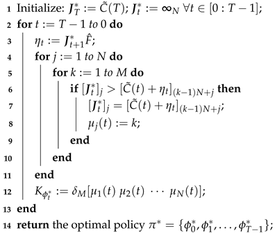3.2. Finite Horizon OTC of MJBCNs with a Penalty for Control Input Changes

Given two control input vectors $U^{\prime }=(U_1^{\prime },U_2^{\prime },\dots ,U_m^{\prime }),U^{″}=(U_1^{″},U_2^{″},\dots ,U_m^{″})\in {\mathcal{D}}^m$, let $u_1={⋉}_{i=1}^m\mathbf{v}\left(U_i^{\prime }\right)\in {\mathsf{\Delta }}_M$ and $u_2={⋉}_{i=1}^m\mathbf{v}\left(U_i^{″}\right)\in {\mathsf{\Delta }}_M$. Similar to the distance formula (6), the distance between $u_1$ and $u_2$ (or between $U^{\prime }$ and $U^{″}$) is given by

$$d_{in}(u_1,u_2)=\sum _{i=1}^m|U_i^{\prime }-U_i^{″}|.$$

Then, the total variation of the control input of MJBCN (2) within the time period of $[0:T-1]$ is expressed as

$$\begin{array}{c}\hfill \tilde{e}(z\left(0\right),\nabla u)=\sum _{t=1}^{T-1}{d}_{in}(u\left(t\right),u(t-1)).\end{array}$$

(15)

Define a penalty factor vector:

$$\tilde{D}=[d_{in}({\delta }_M^1,{\delta }_M^1)d_{in}({\delta }_M^1,{\delta }_M^2)\cdots d_{in}({\delta }_M^1,{\delta }_M^M)d_{in}({\delta }_M^2,{\delta }_M^1)\cdots d_{in}({\delta }_M^M,{\delta }_M^M)],$$

(16)

which satisfies $d_{in}(u_1,u_2)=\tilde{D}⋉u_1⋉u_2,\forall u_1,u_2\in {\mathsf{\Delta }}_M$. Then

$$\tilde{e}(z\left(0\right),\nabla u)=\sum _{t=1}^{T-1}\tilde{D}u\left(t\right)u(t-1).$$

(17)

By performing a weighted sum of (10) and (17), a new objective function denoted by $\widehat{e}(z\left(0\right),y,y^r,\nabla u)$ is obtained as follows:

$$\begin{array}{cc}\hfill \widehat{e}(z\left(0\right),y,y^r,\nabla u)=& \alpha ·e(z\left(0\right),y,y^r)+(1-\alpha )·\tilde{e}(z\left(0\right),\nabla u),\hfill \\ \hfill =& \alpha \left\{\tilde{C}\left(T\right)z\left(T\right)+\sum _{t=1}^{T-1}\tilde{C}\left(t\right)u\left(t\right)z\left(t\right)\right\}+(1-\alpha )\sum _{t=1}^{T-1}\tilde{D}u\left(t\right)u(t-1),\hfill \end{array}$$

(18)

where $0\le \alpha \le 1$. We aim to minimize $\mathbb{E}\left\{\widehat{e}(z\left(0\right),y,y^r,\nabla u)\right\}$ for all $z\left(0\right)\in {\mathsf{\Delta }}_N$. When we are more concerned with the tracking error, we can set $\alpha$ to a larger value. Conversely, if we want to reduce the variation of the control input, we can set $\alpha$ to a smaller value.

Based on the Kronecker product and STP, we can derive

$$\left\{\begin{array}{c}\tilde{C}\left(T\right)z\left(T\right)=\left(\tilde{C}\left(T\right)\otimes {\mathbf{1}}_M^{⊺}\right)z\left(T\right)u(T-1),\hfill \\ \tilde{C}\left(t\right)u\left(t\right)z\left(t\right)=\left(\tilde{C}\left(t\right)\otimes {\mathbf{1}}_M^{⊺}\right)u\left(t\right)z\left(t\right)u(t-1),\hfill \\ \tilde{D}u\left(t\right)u(t-1)=\tilde{D}\left(I_M\otimes {\mathbf{1}}_N^{⊺}\right)u\left(t\right)z\left(t\right)u(t-1).\hfill \end{array}\right.$$

Introduce another instrumental variable $\widehat{z}\left(t\right)$ as follows:

$$\left\{\begin{array}{cc}\hfill \widehat{z}\left(0\right)& =z\left(0\right)\in {\mathsf{\Delta }}_N,\hfill \\ \hfill \widehat{z}\left(t\right)& =z\left(t\right)u(t-1)\in {\mathsf{\Delta }}_{NM},t=1,2,\dots .\hfill \end{array}\right.$$

Define weight factor vectors:

$$\left\{\begin{array}{c}\widehat{C}\left(0\right)={\mathbf{0}}_{NM}^{⊺},\hfill \\ \widehat{C}\left(t\right)=\alpha \left(\tilde{C}\left(t\right)\otimes {\mathbf{1}}_M^{⊺}\right)+(1-\alpha )\tilde{D}(I_M\otimes {\mathbf{1}}_N^{⊺}),t\in [1:T-1],\hfill \\ \widehat{C}\left(T\right)=\alpha \left(\tilde{C}\left(T\right)\otimes {\mathbf{1}}_M^{⊺}\right).\hfill \end{array}\right.$$

(19)

Then we have

$$\widehat{e}(z\left(0\right),y,y^r,\nabla u)=\widehat{C}\left(T\right)\widehat{z}\left(T\right)+\sum _{t=0}^{T-1}\widehat{C}\left(t\right)u\left(t\right)\widehat{z}\left(t\right).$$

(20)

Define two matrices as follows:

$$\left\{\begin{array}{cc}\hfill R& =\widehat{F}\ast \left(I_M\otimes {\mathbf{1}}_N^{⊺}\right),\hfill \\ \hfill L& =\left(\widehat{F}\otimes {\mathbf{1}}_M^{⊺}\right)\ast \left(I_M\otimes {\mathbf{1}}_{NM}^{⊺}\right).\hfill \end{array}\right.$$

(21)

Split R and L into M blocks of the same size: $R=\left[{\overline{R}}_1{\overline{R}}_2\cdots {\overline{R}}_M\right]$ and $L=\left[{\overline{L}}_1{\overline{L}}_2\cdots {\overline{L}}_M\right]$.

Proposition 2.

For any ${\delta }_{NM}^i,{\delta }_N^j\in {\mathsf{\Delta }}_N$ and ${\delta }_M^k\in {\mathsf{\Delta }}_M$,

$$\mathbf{Pr}\{\widehat{z}\left(1\right)={\delta }_{NM}^i\mid \widehat{z}\left(0\right)={\delta }_N^j,u\left(0\right)={\delta }_M^k\}={\left[{\overline{R}}_k\right]}_{ij};$$

for any ${\delta }_{NM}^i,{\delta }_{NM}^j\in {\mathsf{\Delta }}_{NM}$ and ${\delta }_M^k\in {\mathsf{\Delta }}_M$,

$$\mathbf{Pr}\{\widehat{z}(t+1)={\delta }_{NM}^i\mid \widehat{z}\left(t\right)={\delta }_{NM}^j,u\left(t\right)={\delta }_M^k\}={\left[{\overline{L}}_k\right]}_{ij}.$$

Proof. 

The proof is similar to Proposition 1.    □

Next, a policy is in the form of $\widehat{\pi }=\{{\psi }_0,{\psi }_1,\dots ,{\psi }_{T-1}\}$, where ${\psi }_0:{\mathsf{\Delta }}_N\to {\mathsf{\Delta }}_M$ and ${\psi }_t:{\mathsf{\Delta }}_{NM}\to {\mathsf{\Delta }}_M$$\forall t\in [1:T-1]$. There is a $K_{{\psi }_0}\in {\mathcal{L}}_{M\times N}$ such that ${\psi }_0\left(\widehat{z}\left(0\right)\right)=K_{{\psi }_0}\widehat{z}\left(0\right)$, and for each ${\psi }_t$ with $t\ge 1$, there is a $G_{{\psi }_t}\in {\mathcal{L}}_{M\times NM}$ such that ${\psi }_t\left(\widehat{z}\left(t\right)\right)=G_{{\psi }_t}\widehat{z}\left(t\right)$. Once a policy $\widehat{\pi }$ is given, a feedback control is determined as follows:

$$\left\{\begin{array}{c}u\left(0\right)=K_{{\psi }_0}\widehat{z}\left(0\right),\hfill \\ u\left(t\right)=G_{{\psi }_t}\widehat{z}\left(t\right),t\in [1:T-1].\hfill \end{array}\right.$$

(22)

The set of all possible $\widehat{\pi }$ is represented by $\widehat{\mathsf{\Pi }}$.

Minimizing the expected value of (20) by a policy is equivalent to solving an optimization problem as follows:

$$\begin{array}{cc}\hfill \underset{\widehat{\pi }\in \widehat{\mathsf{\Pi }}}{min}\widehat{J}(z\left(0\right),\widehat{\pi })& =\underset{\widehat{\pi }\in \widehat{\mathsf{\Pi }}}{min}\mathbb{E}\left\{\widehat{e}(z\left(0\right),y,y^r,u)\right\},\hfill \\ \hfill {\widehat{\pi }}^{\ast }& =\underset{\widehat{\pi }\in \widehat{\mathsf{\Pi }}}{argmin}\widehat{J}(z\left(0\right),\widehat{\pi }).\hfill \end{array}$$

(23)

${\widehat{\pi }}^{\ast }$ is called an optimal policy if (23) holds for all $z\left(0\right)\in {\mathsf{\Delta }}_N$.

The sub-policies of $\widehat{\pi }=\{{\psi }_0,{\psi }_1,\dots ,{\psi }_{T-1}\}$ are denoted by ${\widehat{\pi }}_k=\{{\psi }_k,{\psi }_{k+1},\dots ,{\psi }_{T-1}\}$, $k\in [1:T-1]$. Denote by ${\widehat{\mathsf{\Pi }}}_k$ the set of all possible ${\widehat{\pi }}_k$. Define the optimal values of the optimization problem (23) and its sub-problems as follows:

$$\left\{\begin{array}{c}{\widehat{J}}_0^{\ast }\left(z\left(0\right)\right)=\underset{\widehat{\pi }\in \widehat{\mathsf{\Pi }}}{min}\widehat{J}(z\left(0\right),\widehat{\pi }),\hfill \\ {\widehat{J}}_k^{\ast }\left(\widehat{z}\left(k\right)\right)=\underset{{\widehat{\pi }}_k\in {\widehat{\mathsf{\Pi }}}_k}{min}\mathbb{E}\left\{\widehat{C}\left(T\right)\widehat{z}\left(T\right)+\sum _{t=k}^{T-1}\widehat{C}\left(t\right)u\left(t\right)\widehat{z}\left(t\right)\right\},k\in [1:T-1],\hfill \\ {\widehat{J}}_T^{\ast }\left(\widehat{z}\left(T\right)\right)=\widehat{C}\left(T\right)\widehat{z}\left(T\right).\hfill \end{array}\right.$$

Similar to Lemma 1, the following lemma is given to determine ${\widehat{J}}_0^{\ast }\left(z\left(0\right)\right)$ through an iterative process for all $z\left(0\right)\in {\mathsf{\Delta }}_N$.

Lemma 2.

For any given $\widehat{z}\left(0\right)\in {\mathsf{\Delta }}_N$,

$${\widehat{J}}_0^{\ast }\left(\widehat{z}\left(0\right)\right)=\underset{u\left(0\right)\in {\mathsf{\Delta }}_M}{min}\mathbb{E}\left\{\widehat{C}\left(0\right)u\left(0\right)\widehat{z}\left(0\right)+{\widehat{J}}_1^{\ast }\left(\widehat{z}\left(1\right)\right)\right\},$$

(24)

and for any given $\widehat{z}\left(t\right)\in {\mathsf{\Delta }}_{NM}$,

$${\widehat{J}}_t^{\ast }\left(\widehat{z}\left(t\right)\right)=\underset{u\left(t\right)\in {\mathsf{\Delta }}_M}{min}\mathbb{E}\left\{\widehat{C}\left(t\right)u\left(t\right)\widehat{z}\left(t\right)+{\widehat{J}}_{t+1}^{\ast }\left(\widehat{z}(t+1)\right)\right\},t\in [1:T-1].$$

(25)

Moreover, if $u\left(0\right)=K_{{\psi }_0}\widehat{z}\left(0\right)$ minimizes the expectation in (24) for all $\widehat{z}\left(0\right)\in {\mathsf{\Delta }}_N$, and $u\left(t\right)=G_{{\varphi }_t^{\ast }}\widehat{z}\left(t\right)$ minimizes the expectation in (25) for all $\widehat{z}\left(t\right)\in {\mathsf{\Delta }}_{NM},t\in [1:T-1]$, then ${\widehat{\pi }}^{\ast }=\{{\psi }_0^{\ast },{\psi }_1^{\ast },\dots ,{\psi }_{T-1}^{\ast }\}$ is an optimal solution of (23).

Define the optimal value vectors:

$$\begin{array}{cc}\hfill {\widehat{\mathit{J}}}_0^{\ast }& =[{\widehat{J}}_0^{\ast }\left({\delta }_N^1\right){\widehat{J}}_0^{\ast }\left({\delta }_N^2\right)\cdots {\widehat{J}}_0^{\ast }\left({\delta }_N^N\right)],\hfill \\ \hfill {\widehat{\mathit{J}}}_t^{\ast }& =[{\widehat{J}}_t^{\ast }\left({\delta }_{NM}^1\right){\widehat{J}}_t^{\ast }\left({\delta }_{NM}^2\right)\cdots {\widehat{J}}_t^{\ast }\left({\delta }_{NM}^{NM}\right)],t\in [1:T].\hfill \end{array}$$

Similarly, given $\widehat{z}\left(0\right)={\delta }_N^i$ in (24) and $\widehat{z}\left(t\right)={\delta }_{NM}^j$ in (25), by Proposition 2,

$$\left\{\begin{array}{c}{\widehat{J}}_0^{\ast }\left({\delta }_N^i\right)=\underset{k\in [1:M]}{min}{\left[{\widehat{\mathit{J}}}_1^{\ast }R\right]}_{(k-1)N+i},\hfill \\ {\widehat{J}}_t^{\ast }\left({\delta }_{NM}^j\right)=\underset{k\in [1:M]}{min}{[\widehat{C}\left(t\right)+{\widehat{\mathit{J}}}_{t+1}^{\ast }L]}_{(k-1)NM+j},t\in [1:T-1].\hfill \end{array}\right.$$

Theorem 2.

The policy ${\widehat{\pi }}^{\ast }$ obtained by Algorithm 2 can minimize the expectation of the objective function (20) for all initial states.

Proof. 

Based on Lemma 2, the proof is similar to Theorem 1.    □

Remark 2.

Algorithm 2 calculates ${\widehat{\mathit{J}}}_t^{\ast }$, $t=T-1,\dots ,0$ recursively and elementwise. The calculation of ${\widehat{\mathit{J}}}_{t+1}^{\ast }L$ takes a time complexity of $O\left(N^2{M}^3\right)$, while lines $4-11$ operate in $O\left(N{M}^2\right)$ time. Thus, lines $2-13$ require $O\left(T{N}^2{M}^3\right)$. The time complexity of the rest is obviously less than $O\left(T{N}^2{M}^3\right)$. Therefore, Algorithm 2 takes at most $O\left(T{N}^2{M}^3\right)$ time complexity. Comparing Algorithm 1 with Algorithm 2, we observe that Algorithm 1 has a lower time complexity. Therefore, if the penalty for control input changes is not considered in the OTC problem, we prioritize using Algorithm 1 to design an optimal strategy ${\pi }^{\ast }$ for MJBCN (2). However, when such a penalty is incorporated, it becomes necessary to employ Algorithm 2 to develop an optimal strategy ${\widehat{\pi }}^{\ast }$.

Algorithm 2: Calculate an optimal solution for (23).

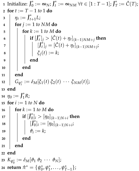Remark 3.

Generally, $u\left(t\right)$ is given from $t=0$. In [16], the virtual variable $u(-1)$ needs to be used. Although time-invariant BCNs were considered, the optimal finite horizon OTC problem with a penalty for control input changes has not been completely addressed. In this paper, we define $\widehat{z}\left(t\right)$ in segmented form, which can effectively solve this problem.

4. Illustrative Examples

Example 1.

Consider an MJBCN model of the form (1) with 3 internal nodes, 1 input node, 2 output nodes and 2 realizations [38], where $f_1^1=X_1$, $f_2^1=\neg X_1\wedge X_3$, $f_3^1=X_2\vee U_1$, $f_1^2=(\neg X_1\wedge X_2)\vee U_1$, $f_2^2=X_1\wedge X_2$, $f_3^2=X_1\wedge X_2$, $h_1=X_1$, $h_2=X_2$. The TPM of $\left\{\sigma \right(t),t\in \mathbb{N}\}$ is assumed to be $P=\left(\begin{array}{cc}0\hfill & 1\hfill \\ 0.6\hfill & 0.4\hfill \end{array}\right)$.

Let $x\left(t\right)={⋉}_{i=1}^3\mathbf{v}\left(X_i\left(t\right)\right)$, $u\left(t\right)=\mathbf{v}\left(U_1\left(t\right)\right)$, $y\left(t\right)=\mathbf{v}\left(Y_1\left(t\right)\right)⋉\mathbf{v}\left(Y_2\left(t\right)\right)$, $\omega \left(t\right)={\delta }_2^{\sigma \left(t\right)}$ and $z\left(t\right)=\omega \left(t\right)x\left(t\right)$. Then, this system can be converted into the form (2) with $F_1={\delta }_8\left[3333575733445768\right]$, $F_2={\delta }_8\left[1144444455884488\right]$ and $H={\delta }_4\left[11223344\right]$. The calculation results of $\widehat{F}$, R, and L are omitted.

A reference trajectory is given in Table 2. By (8), we can obtain

$$\begin{array}{cc}\hfill & C\left(4\right)=\left[2110\right],\hfill \\ \hfill & C\left(1\right)=\left[12011201\right],\hfill \\ \hfill & C\left(2\right)=\left[10211021\right],\hfill \\ \hfill & C\left(3\right)=\left[01120112\right].\hfill \end{array}$$

Next, by (9), we can calculate

$$\begin{array}{cc}\hfill & \tilde{C}\left(4\right)=\left[2211110022111100\right],\hfill \\ \hfill & \tilde{C}\left(1\right)=\left[11220011112200111122001111220011\right],\hfill \\ \hfill & \tilde{C}\left(2\right)=\left[11002211110022111100221111002211\right],\hfill \\ \hfill & \tilde{C}\left(3\right)=\left[00111122001111220011112200111122\right].\hfill \end{array}$$

By Algorithm 1, we can successively obtain

$$\begin{array}{c}{\mathit{J}}_4^{\ast }=\left[2211110022111100\right],\hfill \\ {\mathit{J}}_3^{\ast }=\left[1122213211112222\right],\hfill \\ {\mathit{J}}_2^{\ast }=\left[22114433221.61.63.63.62.62.6\right],\hfill \\ {\mathit{J}}_1^{\ast }=\left[2.62.63.63.63.62.64.63.6333.243.241.241.242.242.24\right],\hfill \\ {\mathit{J}}_0^{\ast }=\left[3.243.243.243.241.242.241.242.242.6562.6563.0563.0563.4563.4563.0563.056\right],\hfill \end{array}$$

and an optimal policy ${\pi }^{\ast }=\{{\varphi }_0^{\ast },{\varphi }_1^{\ast },{\varphi }_2^{\ast },{\varphi }_3^{\ast }\}$ with feedback matrices

$$\begin{array}{c}\hfill K_{{\varphi }_0^{\ast }}={\delta }_2\left[1111111122221122\right],\\ \hfill K_{{\varphi }_1^{\ast }}={\delta }_2\left[1111111111111111\right],\\ \hfill K_{{\varphi }_2^{\ast }}={\delta }_2\left[1111111111111111\right],\\ \hfill K_{{\varphi }_3^{\ast }}={\delta }_2\left[1111111122221122\right].\end{array}$$

Table 2. Reference trajectory 1.

t	1	2	3	4
$Y_1^r$	0	1	1	0
$Y_2^r$	1	0	1	0
$y^r$	${\delta }_4^3$	${\delta }_4^2$	${\delta }_4^1$	${\delta }_4^4$

Next, take the penalty for the control input changes into account. Let $\alpha =0.7$. By (16) and (19), we can obtain $\tilde{D}=\left[0110\right]$ and

$$\begin{array}{c}\widehat{C}\left(4\right)=[1.41.41.41.40.70.70.70.70.70.70.70.70000\hfill \\ \hspace{1em}\hspace{1em}\hspace{1em}1.41.41.41.40.70.70.70.70.70.70.70.70000],\hfill \\ \widehat{C}\left(1\right)=[0.710.711.41.71.41.700.300.30.710.71\hfill \\ \hspace{1em}\hspace{1em}\hspace{1em}0.710.711.41.71.41.700.300.30.710.71\hfill \\ \hspace{1em}\hspace{1em}\hspace{1em}\hspace{1em}10.710.71.71.41.71.40.300.3010.710.7\hfill \\ \hspace{1em}\hspace{1em}\hspace{1em}\hspace{1em}\hspace{1em}10.710.71.71.41.71.40.300.3010.710.7],\hfill \\ \widehat{C}\left(2\right)=[0.710.7100.300.31.41.71.41.70.710.71\hfill \\ \hspace{1em}\hspace{1em}\hspace{1em}0.710.7100.300.31.41.71.41.70.710.71\hfill \\ \hspace{1em}\hspace{1em}\hspace{1em}\hspace{1em}10.710.70.300.301.71.41.71.410.710.7\hfill \\ \hspace{1em}\hspace{1em}\hspace{1em}\hspace{1em}\hspace{1em}10.710.70.300.301.71.41.71.410.710.7],\hfill \\ \widehat{C}\left(3\right)=[00.300.30.710.710.710.711.41.71.41.7\hfill \\ \hspace{1em}\hspace{1em}\hspace{1em}00.300.30.710.710.710.711.41.71.41.7\hfill \\ \hspace{1em}\hspace{1em}\hspace{1em}\hspace{1em}0.300.3010.710.710.710.71.71.41.71.4\hfill \\ \hspace{1em}\hspace{1em}\hspace{1em}\hspace{1em}\hspace{1em}0.300.3010.710.710.710.71.71.41.71.4].\hfill \end{array}$$

By Algorithm 2, we can successively get

$$\begin{array}{cc}\hfill {\widehat{\mathit{J}}}_4^{\ast }=& [1.41.41.41.40.70.70.70.70.70.70.70.70000\hfill \\ & 1.41.41.41.40.70.70.70.70.70.70.70.70000],\hfill \\ \hfill {\widehat{\mathit{J}}}_3^{\ast }=& [0.70.70.70.71.41.41.41.41.41.40.70.72.12.11.41.4\hfill \\ & 10.710.710.710.71.41.41.41.41.71.41.71.4],\hfill \\ \hfill {\widehat{\mathit{J}}}_2^{\ast }=& [1.71.41.71.410.710.72.82.83.12.82.12.12.42.1\hfill \\ & 1.521.821.521.821.241.41.241.42.642.522.642.521.942.11.942.1],\hfill \\ \hfill {\widehat{\mathit{J}}}_1^{\ast }=& [1.942.11.942.12.642.82.642.82.642.521.942.13.343.222.642.8\hfill \\ & 2.3282.6282.3282.6282.4962.7962.4962.7961.0960.981.0960.981.7962.0961.7962.096],\hfill \\ \hfill {\widehat{\mathit{J}}}_0^{\ast }=& [2.4962.4962.4962.4960.981.7960.981.796\hfill \\ & 1.9041.9042.51842.51842.58242.58242.51842.5184],\hfill \end{array}$$

and an optimal policy ${\widehat{\pi }}^{\ast }=\{{\psi }_0^{\ast },{\psi }_1^{\ast },{\psi }_2^{\ast },{\psi }_3^{\ast }\}$ with feedback matrices

$$\begin{array}{cc}\hfill K_{{\psi }_0^{\ast }}={\delta }_2[& 1111212122221122],\hfill \\ \hfill G_{{\psi }_1^{\ast }}={\delta }_2[& 12121212121212121111111112121111],\hfill \\ \hfill G_{{\psi }_2^{\ast }}={\delta }_2[& 12121212121212121111121212121212],\hfill \\ \hfill G_{{\psi }_3^{\ast }}={\delta }_2[& 12121212121212122222222212122222].\hfill \end{array}$$

For each given parameter α, we can always obtain the optimal value of $\mathbb{E}\left\{\widehat{e}(z\left(0\right),y,y^r,u)\right\}$ and an optimal policy by Algorithm 2. However, these optimal values are not directly comparable across different α settings. Therefore, to evaluate the relative merits of different α values, we compare the performance of $\mathbb{E}\left\{e(z\left(0\right),y,y^r)\right\}$ and $\mathbb{E}\left\{\tilde{e}(z\left(0\right),\nabla u)\right\}$ under their respective optimal policies generated by varying α. This approach allows us to select a preferable α value.

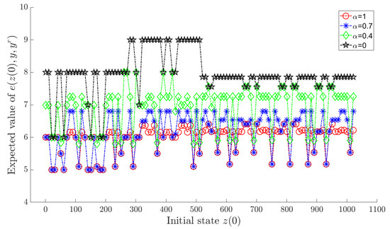
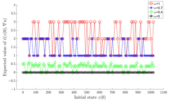
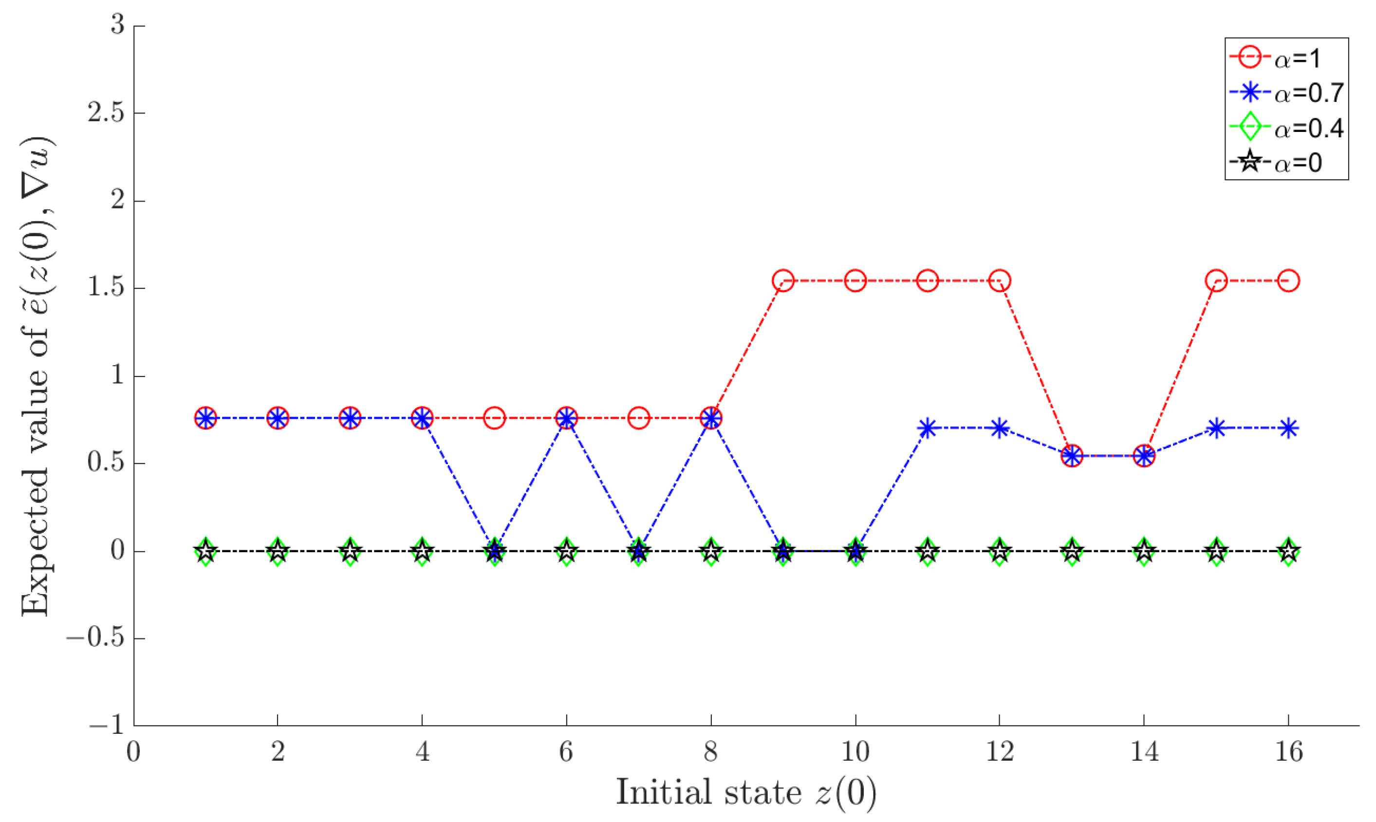
Let α in the objective function (18) take $1,0.7,0.4,0$ sequentially, and an optimal policy can be determined by Algorithm 2 for each value of α. Under each corresponding optimal policy, $\mathbb{E}\left\{e(z\left(0\right),y,y^r)\right\}$ and $\mathbb{E}\left\{\tilde{e}(z\left(0\right),\nabla u)\right\}$ for each $z\left(0\right)\in {\mathsf{\Delta }}_{16}$ are shown in Figure 1 and Figure 2, respectively, where a horizontal axis value of i actually means $z\left(0\right)={\delta }_{16}^i$, $i\in [1:16]$.

Figure 1. $\mathbb{E}\left\{e(z\left(0\right),y,y^r)\right\}$ for each $z\left(0\right)\in {\mathsf{\Delta }}_{16}$ under the optimal policy.

Figure 2. $\mathbb{E}\left\{\tilde{e}(z\left(0\right),\nabla u)\right\}$ for each $z\left(0\right)\in {\mathsf{\Delta }}_{16}$ under the optimal policy.

As shown in the figures, increasing α results in a smaller tracking error, whereas reducing α leads to diminished variation in the control input. This aligns with the design intent of the objective function (18). In comparison, we observe that when $\alpha =0.7$, both the tracking error and variation of control input are effectively maintained at satisfactory levels.

Example 2.

Consider an MJBCN model of the form (1) with 9 internal nodes, 2 input nodes, 3 output nodes, and 2 realizations [39], where

$$\begin{array}{cc}\hfill & f_1^1=f_1^2=\neg X_7\wedge X_3;f_2^1=f_2^2=X_1;f_3^1=f_3^2=\neg U_1;\hfill \\ & f_4^1=f_4^2=X_5\wedge X_6;f_5^1=X_5,f_5^2=X_5\wedge U_2;\hfill \\ & f_6^1=f_6^2=X_1;f_7^1=f_7^2=\neg X_4\wedge \neg X_8;\hfill \\ & f_8^1=f_8^2=X_4\vee X_5\vee X_9;f_9^1=\neg U_1\wedge X_9,f_9^2=X_9;\hfill \\ \hfill & h_1=\neg X_1\wedge X_3;h_2=X_6\vee X_9;h_3=X_2\wedge \neg X_8.\hfill \end{array}$$

The TPM of $\left\{\sigma \right(t),t\in \mathbb{N}\}$ is assumed to be $P=\left(\begin{array}{cc}0.5\hfill & 0.5\hfill \\ 0.3\hfill & 0.7\hfill \end{array}\right)$. Let $x\left(t\right)={⋉}_{i=1}^9\mathbf{v}\left(X_i\left(t\right)\right)$, $u\left(t\right)=\mathbf{v}\left(U_1\left(t\right)\right)⋉\mathbf{v}\left(U_1\left(t\right)\right)$, $y\left(t\right)={⋉}_{j=1}^3\mathbf{v}\left(Y_j\left(t\right)\right)$, $\omega \left(t\right)={\delta }_2^{\sigma \left(t\right)}$ and $z\left(t\right)=\omega \left(t\right)x\left(t\right)$. The transition matrices of this MJBCN are not presented here due to the large dimensionality.

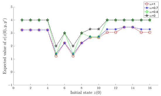
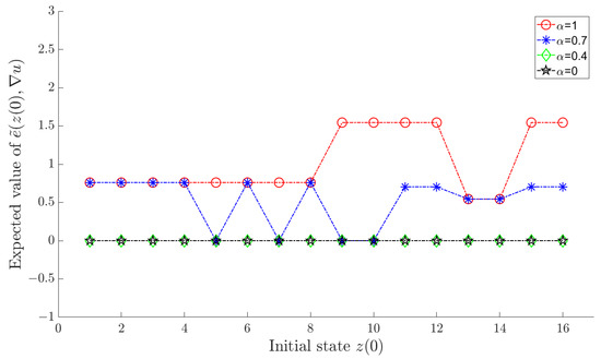
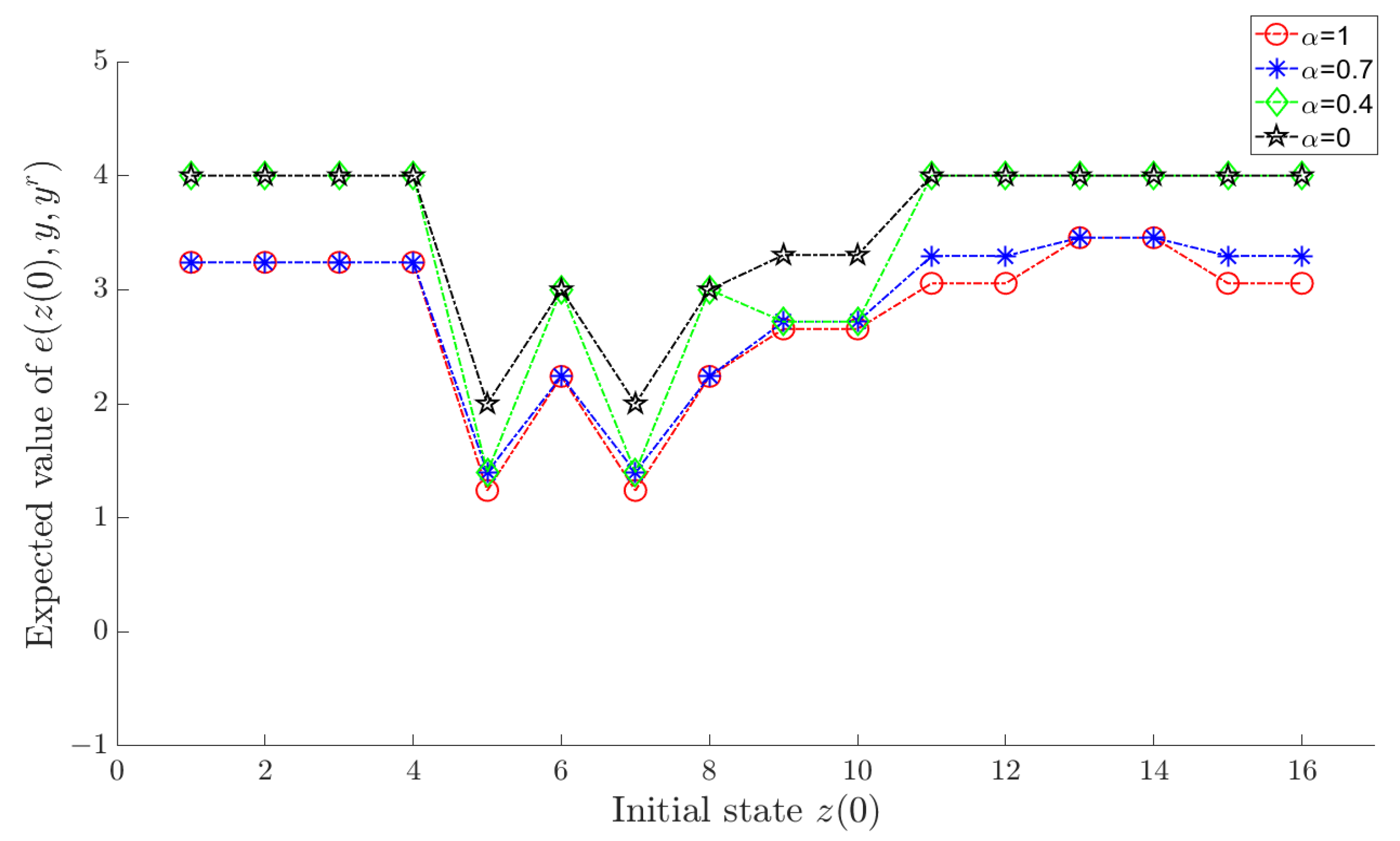
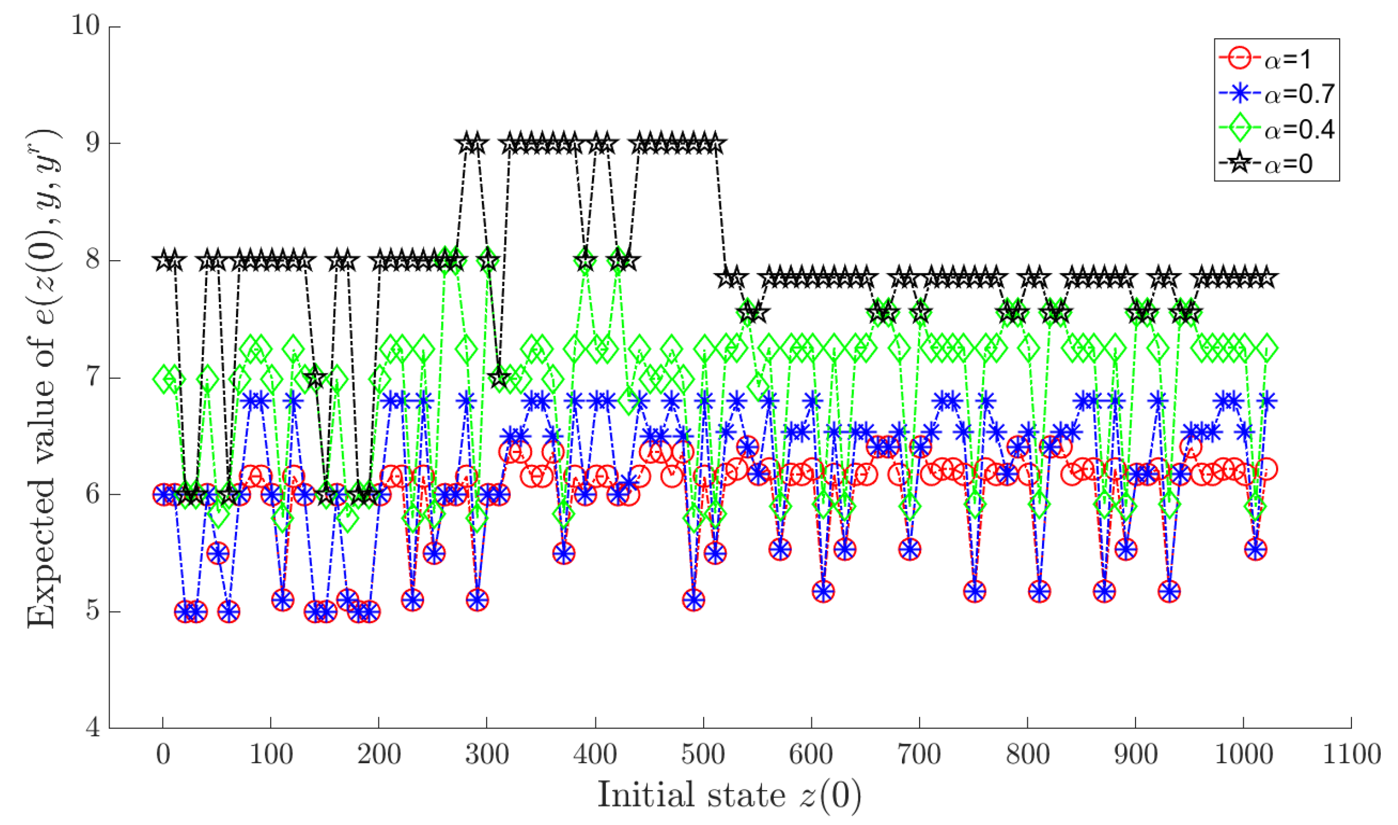
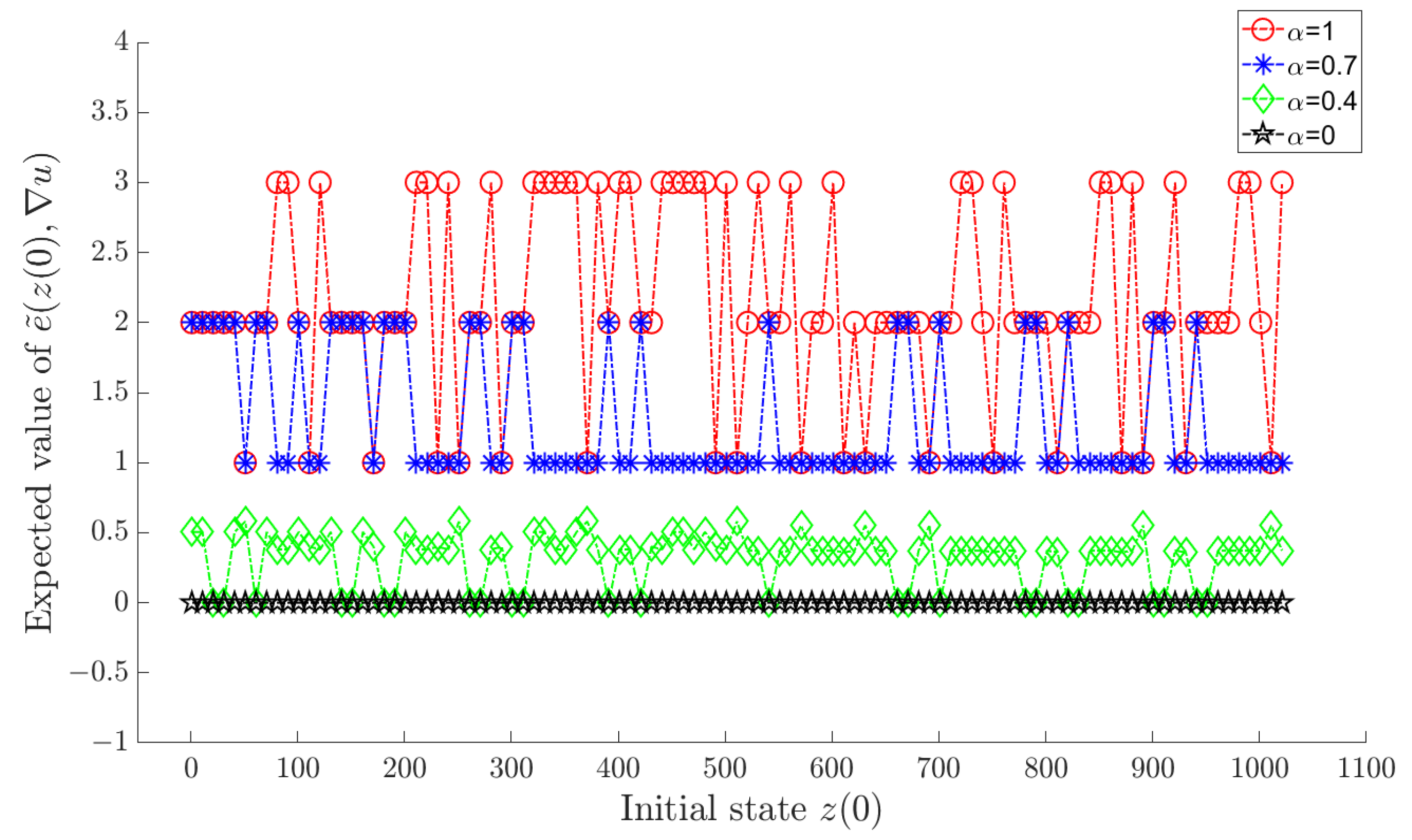
A reference trajectory is given in Table 3. Letting α take $1,0.7,0.4,0$ in (18) sequentially, we can obtain an optimal policy by Algorithm 2 for each value of α. Under each corresponding optimal policy, $\mathbb{E}\left\{e(z\left(0\right),y,y^r)\right\}$ and $\mathbb{E}\left\{\tilde{e}(z\left(0\right),\nabla u)\right\}$ for each $z\left(0\right)\in {\mathsf{\Delta }}_{1024}$ are shown in the Figure 3 and Figure 4, respectively, where a horizontal axis value of i actually means $z\left(0\right)={\delta }_{1024}^i$, $i\in [1:1024]$. To avoid visual clutter, the figures selectively display sparsely sampled data points on the horizontal axis.

Table 3. Reference trajectory 2.

t	1	2	3	4	5	6
$Y_1^r$	1	1	1	0	0	0
$Y_2^r$	1	1	0	1	0	0
$Y_3^r$	0	1	1	0	1	0
$y^r$	${\delta }_8^2$	${\delta }_8^1$	${\delta }_8^3$	${\delta }_8^6$	${\delta }_8^7$	${\delta }_8^8$

Figure 3. $\mathbb{E}\left\{e(z\left(0\right),y,y^r)\right\}$ for each $z\left(0\right)\in {\mathsf{\Delta }}_{1024}$ under the optimal policy.

Figure 4. $\mathbb{E}\left\{\tilde{e}(z\left(0\right),\nabla u)\right\}$ for each $z\left(0\right)\in {\mathsf{\Delta }}_{1024}$ under the optimal policy.

5. Conclusions

This paper studied the minimum error OTC of an MJBCN with respect to a predefined trajectory with a finite length, which was transformed into a dynamic optimization problem in terms of the instrumental variable $z\left(t\right)$. An optimal policy was designed using an algorithm to minimize the expected total tracking error.

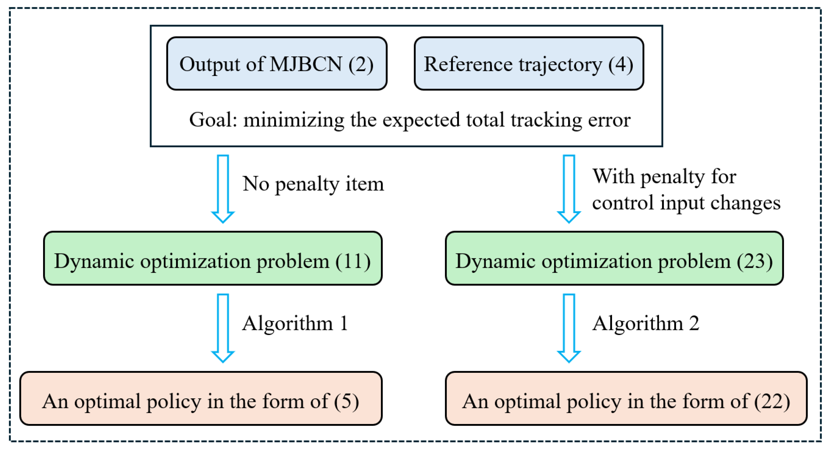
Next, the penalty for control input changes was taken into account. Through the weighted summation of the total tracking error and the total variation of the control input, a new objective function was constructed. The optimal expected value of the objective function and the optimal policy were determined through the dynamic programming of the instrumental variable $\widehat{z}\left(t\right)$. A methodology framework diagram of this paper is provided in Figure 5.

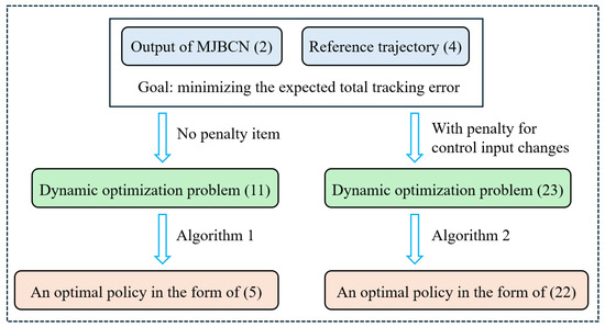
Figure 5. Methodology framework diagram.

Finally, the main results were applied to two simplified biological models. As shown in the examples, the parameter $\alpha$ can be adjusted according to different requirements, and different values of $\alpha$ lead to optimal policies with varying emphasis on the tracking error and the variation of the control input.

References

- Kauffman, S.A. Metabolic stability and epigenesis in randomly constructed genetic nets. J. Theor. Biol. 1969, 22, 437–467. [Google Scholar] [CrossRef] [PubMed]
- Cheng, D.; Qi, H.; Li, Z. Analysis and Control of Boolean Networks: A Semi-Tensor Product Approach; Springer: London, UK, 2011. [Google Scholar]
- Liu, W.; Fu, S.; Zhao, J. Set stability and set stabilization of Boolean control networks avoiding undesirable set. Mathematics 2021, 9, 2864. [Google Scholar] [CrossRef]
- Sun, Q.; Li, H. Robust stabilization of impulsive Boolean control networks with function perturbation. Mathematics 2022, 10, 4029. [Google Scholar] [CrossRef]
- Deng, L.; Cao, X.; Zhao, J. One-bit function perturbation impact on robust set stability of Boolean networks with disturbances. Mathematics 2024, 12, 2258. [Google Scholar] [CrossRef]
- Tang, T.; Ding, X.; Lu, J.; Liu, Y. Improved criteria for controllability of Markovian jump Boolean control networks with time-varying state delays. IEEE Trans. Autom. Control 2024, 69, 7028–7035. [Google Scholar] [CrossRef]
- Li, Y.; Feng, J.-E.; Wang, B. Observability of singular Boolean control networks with state delays. J. Franklin Inst. 2022, 359, 331–351. [Google Scholar] [CrossRef]
- Li, Y.; Li, H. Relation coarsest partition method to observability of probabilistic Boolean networks. Inf. Sci. 2024, 681, 121221. [Google Scholar] [CrossRef]
- Chen, H.; Wang, Z.; Liang, J.; Li, M. State estimation for stochastic time-varying Boolean networks. IEEE Trans. Autom. Control 2020, 65, 5480–5487. [Google Scholar] [CrossRef]
- Chen, H.; Wang, Z.; Shen, B.; Liang, J. Model evaluation of the stochastic Boolean control networks. IEEE Trans. Autom. Control 2022, 67, 4146–4153. [Google Scholar] [CrossRef]
- Li, Y.; Li, H.; Xiao, G. Luenberger-like observer design and optimal state estimation of logical control networks with stochastic disturbances. IEEE Trans. Autom. Control 2023, 68, 8193–8200. [Google Scholar] [CrossRef]
- Li, B.; Pan, Q.; Zhong, J.; Xu, W. Long-run behavior estimation of temporal Boolean networks with multiple data losses. IEEE Trans. Neural Netw. Learn. Syst. 2024, 35, 15004–15011. [Google Scholar] [CrossRef]
- Li, B.; Lu, J.; Xu, W.; Zhong, J. Lossless state compression of Boolean control networks. IEEE Trans. Autom. Control 2024, 69, 4166–4173. [Google Scholar] [CrossRef]
- Li, H.; Wang, Y.; Xie, L. Output tracking control of Boolean control networks via state feedback: Constant reference signal case. Automatica 2015, 59, 54–59. [Google Scholar] [CrossRef]
- Li, H.; Xie, L.; Wang, Y. Output regulation of Boolean control networks. IEEE Trans. Autom. Control 2017, 62, 2993–2998. [Google Scholar] [CrossRef]
- Zhang, Z.; Leifeld, T.; Zhang, P. Finite horizon tracking control of Boolean control networks. IEEE Trans. Autom. Control 2018, 63, 1798–1805. [Google Scholar] [CrossRef]
- Zhao, Y.; Zhao, X.; Fu, S.; Xia, J. Robust output tracking of Boolean control networks over finite time. Mathematics 2022, 10, 4078. [Google Scholar] [CrossRef]
- Gao, Z.; Feng, J.-E. Research status of nonlinear feedback shift register based on semi-tensor product. Mathematics 2022, 10, 3538. [Google Scholar] [CrossRef]
- Wang, S.; Li, H. Resolution of fuzzy relational inequalities with Boolean semi-tensor product composition. Mathematics 2021, 9, 937. [Google Scholar] [CrossRef]
- Shmulevich, I.; Dougherty, E.R.; Zhang, W. From Boolean to probabilistic Boolean networks as models of genetic regulatory networks. Proc. IEEE 2002, 90, 1778–1792. [Google Scholar] [CrossRef]
- Shmulevich, I.; Dougherty, E.R.; Kim, S.; Zhang, W. Probabilistic Boolean networks: A rule-based uncertainty model for gene regulatory networks. Bioinformatics 2002, 18, 261–274. [Google Scholar] [CrossRef]
- Kim, S.; Li, H.; Dougherty, E.R.; Cao, N.; Chen, Y.; Bittner, M.; Suh, E.B. Can Markov chain models mimic biological regulation? J. Biol. Syst. 2002, 10, 337–357. [Google Scholar] [CrossRef]
- Meng, M.; Xiao, G.; Zhai, C.; Li, G. Controllability of Markovian jump Boolean control networks. Automatica 2019, 106, 70–76. [Google Scholar] [CrossRef]
- Chen, B.; Cao, J.; Lu, G.; Rutkowski, L. Stabilization of Markovian jump Boolean control networks via sampled-data control. IEEE Trans. Cybern. 2022, 52, 10290–10301. [Google Scholar] [CrossRef]
- Chen, B.; Cao, J.; Lu, G.; Rutkowski, L. Stabilization of Markovian jump Boolean control networks via event-triggered control. IEEE Trans. Autom. Control 2023, 68, 1215–1222. [Google Scholar] [CrossRef]
- Melhem, K.; Wang, W. Global output tracking control of flexible joint robots via factorization of the manipulator mass matrix. IEEE Trans. Robot. 2009, 25, 428–437. [Google Scholar] [CrossRef]
- Al-Hiddabi, S.A.; McClamroch, N.H. Tracking and maneuver regulation control for nonlinear nonminimum phase systems: Application to flight control. IEEE Trans. Control Syst. Technol. 2002, 10, 780–792. [Google Scholar] [CrossRef]
- Li, H.; Wang, Y.; Guo, P. State feedback based output tracking control of probabilistic Boolean networks. Inf. Sci. 2016, 349–350, 1–11. [Google Scholar] [CrossRef]
- Chen, B.; Cao, J.; Luo, Y.; Rutkowski, L. Asymptotic output tracking of probabilistic Boolean control networks. IEEE Trans. Circuits Syst. I. Reg. Papers 2020, 67, 2780–2790. [Google Scholar] [CrossRef]
- Abdollahi, J.; Dubljevic, S. Lipid production optimization and optimal control of heterotrophic microalgae fed-batch bioreactor. Chem. Eng. Sci. 2012, 84, 619–627. [Google Scholar] [CrossRef]
- Zhang, Q.; Feng, J.-E.; Jiao, T. Finite horizon tracking control of probabilistic Boolean control networks. J. Franklin Inst. 2021, 358, 9909–9928. [Google Scholar] [CrossRef]
- Zhang, A.; Li, L.; Li, Y.; Lu, J. Finite-time output tracking of probabilistic Boolean control networks. Appl. Math. Comput. 2021, 411, 126413. [Google Scholar] [CrossRef]
- Li, Y.; Li, H.; Xiao, G. Optimal control for reachability of Markov jump switching Boolean control networks subject to output trackability. Int. J. Control 2025, 98, 200–207. [Google Scholar] [CrossRef]
- Khatri, C.G.; Rao, C.R. Solutions to some functional equations and their applications to characterization of probability distributions. Sankhyā Indian J. Stat. A 1968, 30, 167–180. [Google Scholar]
- Li, C.; Zhang, X.; Feng, J.-E.; Cheng, D. Transition analysis of stochastic logical control networks. IEEE Trans. Autom. Control 2024, 69, 1226–1233. [Google Scholar] [CrossRef]
- Liu, Z.; Wang, Y.; Li, H. Two kinds of optimal controls for probabilistic mix-valued logical dynamic networks. Sci. China Inf. Sci. 2014, 57, 1–10. [Google Scholar] [CrossRef]
- Wu, Y.; Shen, T. An algebraic expression of finite horizon optimal control algorithm for stochastic logical dynamical systems. Syst. Control Lett. 2015, 82, 108–114. [Google Scholar] [CrossRef]
- Meng, M.; Liu, L.; Feng, G. Stability and l1 gain analysis of Boolean networks with Markovian jump parameters. IEEE Trans. Autom. Control 2017, 62, 4222–4228. [Google Scholar] [CrossRef]
- Acernese, A.; Yerudkar, A.; Glielmo, L.; Del Vecchio, C. Reinforcement learning approach to feedback stabilization problem of probabilistic Boolean control networks. IEEE Control Syst. Lett. 2021, 5, 337–342. [Google Scholar] [CrossRef]
Disclaimer/Publisher’s Note: The statements, opinions and data contained in all publications are solely those of the individual author(s) and contributor(s) and not of MDPI and/or the editor(s). MDPI and/or the editor(s) disclaim responsibility for any injury to people or property resulting from any ideas, methods, instructions or products referred to in the content. |
© 2025 by the authors. Licensee MDPI, Basel, Switzerland. This article is an open access article distributed under the terms and conditions of the Creative Commons Attribution (CC BY) license (https://creativecommons.org/licenses/by/4.0/).