Abstract
This study proposes a novel nonlinear adaptive fuzzy hybrid sliding mode (AFHSM) control strategy for the precise trajectory tracking of autonomous mobile robots (AMRs) equipped with four Mecanum wheels. The control design addresses the inherent complexities of such platforms, which include strong system nonlinearities, significant parametric uncertainties, torque saturation effects, and external disturbances that can adversely affect dynamic performance. Unlike conventional approaches that rely on model linearization or dimension reduction, the proposed AFHSM control retains the full nonlinear characteristics of the system to ensure accurate and robust control. The controller is systematically derived from the trajectory-tracking error dynamics between the AMR and the desired trajectory (DT). It integrates higher-order sliding mode (SM) control, fuzzy logic inference, and adaptive learning mechanisms to enable real-time compensation for model uncertainties and external perturbations. In addition, a saturation handling mechanism is incorporated to ensure that the control signals remain within feasible limits, thereby preserving actuator integrity and improving practical applicability. The stability of the closed-loop nonlinear system is rigorously established through the Lyapunov theory, guaranteeing the asymptotic convergence of tracking errors. Comprehensive simulation studies conducted under severe conditions with up to 60 percent model uncertainty confirm the superior performance of the proposed method compared to classical SM control. The AFHSM control consistently achieves lower trajectory and heading errors while generating smoother control signals with reduced torque demand. This improvement enhances tracking precision, suppresses chattering, and significantly increases energy efficiency. These results validate the effectiveness of the AFHSM control approach as a robust and energy-aware control solution for AMRs operating in highly uncertain and dynamically changing environments.
Keywords:
adaptive fuzzy; sliding mode control; trajectory tracking; Lyapunov analysis; energy consumption MSC:
37M05
1. Introduction
In recent decades, autonomous mobile robots (AMRs) have garnered significant attention due to their widespread applications across various domains, including healthcare, agriculture, military, entertainment, household services, commerce, disaster response, and industry. These applications encompass medical assistance robots, agricultural operation robots, surveillance and inspection robots, entertainment companion robots, household cleaning robots, navigation service robots, disaster response robots, and autonomous material handling robots. With the expansion of application scenarios, the ability of AMRs to achieve precise motion control in complex and dynamically changing environments has become increasingly critical. Consequently, the development of high-precision and robust trajectory-tracking control techniques has emerged as a key research challenge in AMR technology. Currently, most AMRs adopt either a four-wheel drive system or a two-wheel drive system with auxiliary omnidirectional wheels to meet the requirements of different operational environments. One of the fundamental challenges in AMR design is ensuring accurate trajectory-tracking control, enabling the robot to follow the desired trajectory (DT) effectively while maintaining stability and precision, even in the presence of system uncertainties or external disturbances. Therefore, designing efficient trajectory-tracking control strategies for AMRs has become a focal point for researchers.
This study reviews and synthesizes the existing literature on AMR trajectory-tracking control, covering various methodologies, including model predictive control (MPC) [1,2], linear quadratic regulator (LQR) control [3,4], neural network control [5,6,7,8], fuzzy control [9,10,11,12,13,14], SM control [15,16,17,18,19,20,21,22], proportional–integral–derivative (PID) control [23,24,25,26,27], backstepping control [28,29,30,31,32], finite-time control [33,34,35], model-free adaptive control [36,37,38], exponential trajectory-tracking control [39], feedback linearization control [40,41,42], and H2 control [43,44,45,46]. These studies primarily focus on trajectory-tracking control design for two-wheel or four-wheel AMRs equipped with either Mecanum wheels or conventional wheels, based on both simulations and experimental validations.
Some studies [3,4,6,8,19,23,25,26,27,29,39,41,43,44] propose trajectory-tracking control methods under the assumption of ideal conditions, where model uncertainties and external disturbances are not considered. However, in real-world applications, parameters such as the mass and moment of inertia of AMRs may vary over time due to changes in payload and energy consumption. If these influencing factors are neglected, the trajectory-tracking performance may deteriorate significantly. For instance, conventional trajectory-tracking methods may struggle to compensate for unknown external disturbances or variations in payload, leading to substantial trajectory errors or even stability issues. Furthermore, studies [43,44] introduce a nonlinear optimal control solution for AMRs based on coordinate transformation, which provides an analytical solution under fixed system parameters. However, solving the nonlinear optimal trajectory-tracking problem for AMRs is highly challenging, particularly in deriving closed-form analytical solutions. The H2 control approach presented in [43,44] suggests that an optimal trajectory-tracking analytical solution can be obtained for AMRs with fixed parameters by appropriately formulating the mathematical model. Nevertheless, fixed-parameter AMRs are exceptional cases, as practical AMRs typically exhibit time-varying system parameters due to payload fluctuations, energy dissipation, and other factors. Consequently, trajectory-tracking solutions derived under fixed-parameter assumptions may not be applicable in real-world scenarios, especially in complex environments with unknown external disturbances.
To address the challenges posed by model uncertainties and external disturbances in AMR trajectory tracking, recent studies [5,7,9,10,11,12,13,14,15,16,18,21,30,31,33,34,36,37,38,45,46] have explored adaptive control strategies to enhance robustness and adaptability. The core concept of adaptive control is to dynamically adjust control strategies based on system parameter variations, thereby maintaining satisfactory tracking performance in uncertain environments. Although adaptive control methods have demonstrated promising capabilities in handling model uncertainties, improper design may lead to increased computational burden, excessive control oscillations, and higher energy consumption. Therefore, designing an AMR trajectory-tracking control method that simultaneously achieves high performance and low computational costs remains a significant research challenge.
Adaptive fuzzy fault-tolerant control (FFTC) has seen significant progress in addressing nonlinear systems affected by actuator faults, unknown control directions, and external disturbances. In [47], an indirect adaptive fuzzy controller incorporating a Nussbaum-type gain effectively managed to control direction uncertainty and actuator failures while avoiding singularities and parameter projection—offering a streamlined yet effective solution for SISO systems. Reference [48] proposes a direct adaptive control strategy with a two-layer architecture, improving robustness against fuzzy approximation errors and exogenous disturbances. Extending to MIMO systems, ref. [49] presents a scalable FFTC framework capable of handling state-dependent actuator faults and unknown control signs by integrating fuzzy logic with Nussbaum-based adaptive techniques. Collectively, these contributions underscore the efficacy of combining fuzzy approximation with adaptive and robust control mechanisms to ensure resilient performance under complex uncertainties.
Recent theoretical developments have focused on improving the stabilization of complex systems under time delay and input constraints. Delay-kernel-dependent methods have been proposed to address the saturated control problem of linear systems with mixed delays, where distributed delay kernels are integrated into Lyapunov–Krasovskii functionals and polytopic representations. These approaches enable less conservative stability criteria and effectively mitigate the dimensionality issues associated with classical delay-dependent formulations [50]. In parallel, distributed-delay-dependent strategies have been applied to interval type-2 fuzzy systems with stochastic network-induced delays and actuator saturation. By modeling delays using probability density functions and incorporating actuator constraints into the polytopic structure, these methods yield more practical stability conditions and broader estimations of the domain of attraction [51]. Together, these advancements provide valuable tools for designing robust controllers in systems affected by uncertainties, delays, and nonlinear input constraints.
Motivated by these considerations, this study proposes an AFHSM control method for four-wheel Mecanum-wheeled mobile robots to improve trajectory-tracking accuracy and control performance under model uncertainties and external disturbances. The AFHSM control method integrates the strong robustness of SM control with the adaptive capability of fuzzy logic, effectively mitigating the adverse effects of system uncertainties while reducing control output oscillations and energy consumption. As a result, this approach enhances AMR motion stability and execution efficiency. To validate the effectiveness of the proposed method, this study conducts simulation-based trajectory-tracking performance evaluations, comparing the AFHSM control method with the SM control method. The results demonstrate that under various uncertainty and disturbance conditions, the AFHSM control method significantly outperforms the SM control method in terms of control response, trajectory-tracking accuracy, adaptability, and energy efficiency.
An AFHSM control strategy is developed to compensate for uncertainties in system parameters by integrating fuzzy logic approximation, adaptive parameter tuning, and hybrid SM control. The fuzzy logic system approximates unknown nonlinearities, enhancing the generalization capability under uncertain conditions. An adaptive learning mechanism continuously updates the control parameters to accommodate time-varying dynamics. Meanwhile, the hybrid SM framework improves robustness and suppresses chattering, ensuring accurate trajectory-tracking and closed-loop stability in dynamic environments.
This study addresses the challenges posed by nonlinear dynamics, time-varying uncertainties, and external disturbances commonly encountered in real-world AMR applications by introducing a novel AFHSM control strategy for Mecanum-wheeled platforms. The proposed method aims to achieve robust and precise trajectory tracking without resorting to system simplifications, while simultaneously improving control adaptability and energy efficiency. By combining fuzzy approximation, SM robustness, and adaptive learning mechanisms, the controller dynamically compensates for modeling inaccuracies and external perturbations, thereby ensuring closed-loop stability and enhanced performance in complex and uncertain operating environments.
The novelty of this study lies in the development of a nonlinear AFHSM control framework tailored for four-wheel Mecanum-wheeled AMRs, which fully preserves system nonlinearities without relying on linearization or model reduction. Unlike existing methods that typically assume fixed parameters or neglect external disturbances, the proposed controller integrates fuzzy approximation and adaptive learning to handle dynamic uncertainties, actuator variations, and environmental disturbances in real time. Furthermore, the design enhances energy efficiency while maintaining high tracking precision, offering a practical and robust solution for real-world AMR applications where model variability and disturbance rejection are critical.
In light of the limitations found in conventional trajectory-tracking approaches—particularly their sensitivity to modeling uncertainties, actuator faults, and external disturbances—this study presents a novel AFHSM control scheme for AMRs with four Mecanum wheels. The originality of this work lies in several key aspects:
First, the proposed AFHSM controller is derived directly from the nonlinear trajectory-tracking error dynamics without resorting to system linearization or dimension reduction, thereby preserving the full nonlinear behavior of the AMR. Second, the control strategy integrates the robustness of the SM control with the adaptivity of fuzzy logic systems, enabling dynamic compensation for system uncertainties and time-varying disturbances. Unlike traditional SM control, the proposed design avoids chattering and singularity problems through a smooth adaptive mechanism. Third, a Lyapunov–Krasovskii-based stability framework is constructed to rigorously verify the asymptotic stability of the closed-loop system while ensuring that all internal signals remain bounded. Finally, comparative simulation studies against conventional SM control demonstrate the superior performance of the proposed AFHSM controller in terms of trajectory accuracy, adaptability, disturbance rejection, and energy efficiency. These contributions offer a robust and energy-conscious trajectory-tracking solution for AMRs operating in uncertain and dynamically changing environments.
To facilitate clarity and consistency throughout the paper, the notation and descriptions of the mathematical symbols employed in the proposed control framework are summarized in Table 1.

Table 1.
Notation and descriptions of mathematical symbols.
The structure of this paper is as follows: Section 1 presents an overview of the background and related works; Section 2 formulates the dynamic equations of the AMR; Section 3 details the design of the nonlinear AFHSM control; Section 4 provides simulation verification and a discussion of the results based on the proposed method; finally, Section 5 concludes the study by highlighting the key findings.
2. Dynamic Equations of the AMR
This section presents the dynamic equations of the AMR and explains the significance of each parameter associated with the four Mecanum wheels equipped on the AMR. Each Mecanum wheel contains a set of passive rollers, which rotate around the hub of the robot at a 45° angle relative to the robot’s central axis. Figure 1 illustrates the kinematic diagram of the AMR equipped with four Mecanum wheels [46]. The relevant parameters and dynamic equations of the AMR will be discussed in detail below.
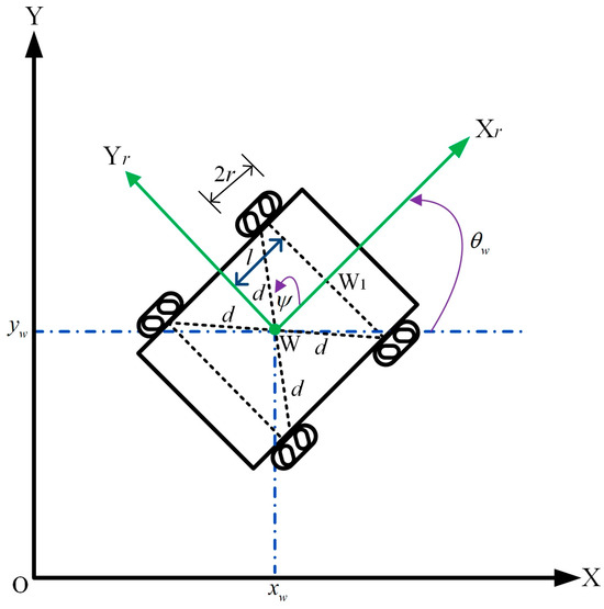
Figure 1.
Kinematic diagram of the AMR equipped with four Mecanum wheels.
Figure 1 presents the kinematic diagram of the AMR equipped with four Mecanum wheels, defining the following parameters: X and Y denote the global coordinate system, while Xr and Yr represent the moving coordinate system centered at point W of the AMR. The parameter specifies the distance between points W and W1, whereas indicates the separation between the central point W and each Mecanum wheel. Additionally, defines the AMR’s rotation angle, and describes the angle between the roller axis and the wheel plane. The AMR’s global position and orientation are compactly described by the state vector , where and denote the Cartesian coordinates of the AMR in the inertial frame, and denotes its global heading angle.
As depicted in Figure 1, the AMR typically moves along the direction of the driving wheel axes. Its dynamic equations and related parameters are described by Equations (1)–(10) [46].
where
In this formulation, denotes the inertia matrix, while represents the Coriolis and centripetal matrix. The generalized velocity and acceleration vectors are denoted by and , respectively. The input transformation matrix is represented by , whereas defines the friction direction matrix. Additionally, corresponds to the wheel’s rotational speed, and characterizes the friction effect matrix. The parameter r indicates the wheel radius, represents the torque of the force vector, and accounts for external disturbances. Moreover, and denote the wheel and platform masses, respectively, while and correspond to the wheel and platform moments of inertia. In this study, the AMR parameters (, , ) are affected by uncertainties arising from model perturbations.
3. Design of Nonlinear Adaptive Fuzzy Hybrid Sliding Mode Control
In this section, a nonlinear AFHSM control method with saturation is designed for the trajectory tracking of AMR. The stability of the nonlinear closed-loop system is rigorously proven through Lyapunov analysis. The following discussion will provide a detailed explanation of the AFHSM-based trajectory-tracking control design.
In this study, the DT is assumed to be a twice continuously differentiable function . Additionally, and represent the velocity and acceleration vector of the trajectory , respectively. Based on these definitions, the trajectory-tracking error between the AMR and the DT can be formulated as the following equation.
where
To develop the proposed trajectory-tracking control method for the AMR, the dynamics of the AMR in Equation (1) can be reformulated into the state-space representation, as expressed in Equations (13) and (14).
where
To simplify the state-space formulation in Equation (14) for the subsequent design of the AFHSM control method, the state-space representation can be reformulated as follows.
where
The first tracking error is defined as the deviation between the navigated position and angle and their desired value . Similarly, the second tracking error represents the difference between the navigated linear and angular velocity and their desired counterpart , as expressed in Equations (21) and (22).
where
Furthermore, the sliding surface is chosen as follows:
The rationale for this structure lies in enhancing robustness and convergence speed. By combining the error and its derivative, the sliding surface not only drives the tracking error to zero but also suppresses oscillations and improves transient performance. Moreover, this structure facilitates the use of higher-order SM control laws, such as the super-twisting algorithm, which reduces chattering and ensures finite-time convergence even under bounded uncertainties and disturbances.
Therefore, the selected structures of and are deliberately designed to enhance the robustness and performance of the control system.
In this study, saturation limits are incorporated into each control law and torque input to constrain the applied force, ensuring that the system operates within a safe range while enhancing its stability and efficiency. The constrained local control law is defined as follows:
Let be defined as the unidentified discrepancy between the control law and the constrained control law . Therefore, the relationship between these two control laws can be further expressed as follows:
where
The term is defined in the following section, while represents a tunable positive parameter that constrains the range of the developed control law .
Additionally, the constrained control law can be decomposed into the control law and the unidentified control discrepancies .
By substituting Equations (28) and (29) into Equation (17), Equation (17) can be reformulated as follows:
where represents the total disturbance of the system.
In order to counteract the total disturbance , a fuzzy-based estimator is formulated as follows:
Here, denotes the parameter matrix, and represents the parameter of the updated law, both of which are defined as follows:
The quantity, N, of the If-Then rules is adjustable. As the number of If-Then rules grows, computational complexities in their implementation also rise.
Moreover, the optimal parameter searched by the update law is defined as follows to govern the update process.
Here, represents the Euclidean norm, while denotes the set of .
Consequently, the optimal estimate can be expressed in terms of the optimal parameter from Equation (38) and the parameter matrix from Equation (33) as follows:
The approximation error between the total disturbance in Equation (31) and the optimal estimation in Equation (39) can be expressed as follows:
Additionally, the approximation error of parameter between the update law parameter in Equation (38) and the optimal update law parameter in Equation (38) can be described as follows:
In order to design the selected control law , the error dynamics are formulated as follows:
Thus, the selected control law can be determined as follows:
Substituting the control law selected in Equation (44), Equations (40) and (41) can be substituted into the error dynamics of Equation (43), as illustrated below:
To examine the convergence behavior of the control law, a Lyapunov candidate function is chosen as follows:
The derivative of the Lyapunov candidate function is expressed as follows:
Referring to the designated sliding surface in Equations (25) and (26), its derivative can be determined as follows.
By incorporating Equations (21), (25) and (45) together with the time derivatives of the sliding surfaces defined in Equations (48) and (49), the time derivative of the proposed Lyapunov candidate function can be systematically derived, and expressed as follows.
According to the trace property, the trace of the matrix is governed by the following equation.
Leveraging the trace property in Equation (51), the time derivative of the Lyapunov candidate in Equation (50) can be further simplified as follows.
Accordingly, the update law for the parameter can be defined as follows.
Substituting the parameter adaptation law into the time derivative of the Lyapunov candidate function given in Equation (52) yields a second simplified expression, as shown in Equation (54).
Supposing that the designable parameter lies beyond the range of the approximation error , the following is calculated:
where the designable variable is determined based on each specific case.
Based on the previous derivation, the derivative of the Lyapunov candidate function in Equation (54) is shown to be negative, as indicated in Equation (56). This result implies that the system’s energy or tracking error gradually decreases over time, leading to system stabilization and ultimately reaching the desired target. Therefore, the designed control law not only guarantees system stability but also ensures convergence, meaning that the system state progressively approaches the equilibrium point or reference trajectory, thereby enhancing the reliability and performance during operation.
The Lyapunov candidate function shown in Equation (46) is carefully constructed to ensure the convergence and stability of the closed-loop system under the designed control law. This functional comprises the quadratic terms of the sliding surfaces and , as well as a trace term involving the parameter estimation error , which collectively captures both the system’s dynamic behavior and adaptation performance.
The inclusion of the trace term is critical in quantifying the parameter estimation error, thereby enabling the formulation of an adaptive control strategy that ensures the boundedness of the estimation process. Moreover, the time derivative of the Lyapunov candidate function in Equation (47) explicitly accounts for the dynamics of the sliding surfaces defined in Equations (48) and (49), resulting in the compact form of Equation (50), which simplifies the stability analysis and ensures asymptotic convergence.
The chosen Lyapunov candidate functional was purposefully constructed to exploit the trace properties of the matrix calculus, as demonstrated in Equation (51), thereby streamlining the stability analysis and effectively addressing parameter uncertainties. This specific structure was selected to rigorously establish closed-loop stability, enhance robustness against modeling inaccuracies, and facilitate the formulation of a smooth adaptive control law.
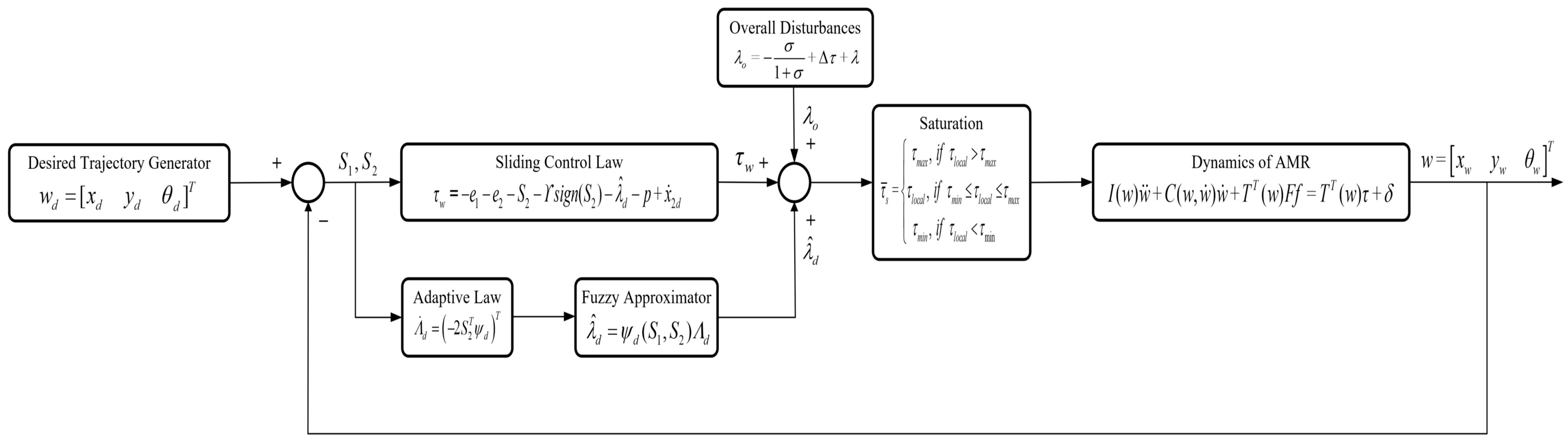
The overall structure of the proposed AFHSM control scheme is illustrated in Figure 2. It summarizes the integration of desired trajectory generation, SM control, adaptive fuzzy estimation, and torque saturation handling within the AMR dynamic model. This architecture highlights how the designed control components collaboratively ensure robust and accurate trajectory tracking under uncertainties and external disturbances.
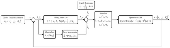
Figure 2.
Control architecture of the proposed nonlinear AFHSM controller for AMR trajectory tracking.
4. Simulation Verification and Results Discussion
In this section, we present the simulation and validation of the trajectory-tracking performance of the SM and AFHSM control methods for triangle-shaped and convex-shaped DTs using MATLAB R2024b software. The following subsections provide a detailed discussion of the parameters for AMR and assumptions on model uncertainties, the design of the membership functions and fuzzy logic system, and the analysis of the simulation results.
4.1. Parameters for AMR and Assumptions on Model Uncertainties
This section presents the configuration parameters of the AMR and the assumed values for model uncertainties. First, the configuration parameters of the controlled AMR, as shown in Figure 1, are listed, with the corresponding parameter values provided in Table 2. Subsequently, we define the assumed parameter values intended to address model uncertainties. These assumptions play a crucial role in ensuring the accuracy and reliability of the results when validating the trajectory-tracking performance of the SM and AFHSM control methods for the desired triangle-shaped and convex-shaped trajectories during the simulation process.
Table 2.
The configuration parameters of the controlled AMR [46].
For the controlled AMR, model uncertainties were assumed to be 60% of the distance from W to each wheel , the AMR platform mass , and the AMR platform inertia , respectively. These assumptions were made to simulate practical scenarios where the AMR carries different loads, reflecting the potential variations and uncertainties that may arise due to load changes or external disturbances during operation. Specifically, these model uncertainties account for parameter fluctuations that may occur under varying operational conditions. By incorporating these assumptions into the simulation, we aimed to validate the robustness and effectiveness of the SM and AFHSM control methods in different scenarios, thereby enhancing the reliability of the model for real-world applications.
4.2. Design of the Membership Functions and Fuzzy Logic System
In this study, Gaussian functions were selected as the membership functions due to their favorable mathematical properties, which effectively handle model uncertainties and nonlinearities in fuzzy logic systems. The advantage of Gaussian functions lies in their smoothness and differentiability, enabling more precise fuzzy inference in control systems, particularly when designing a nonlinear AFHSM system. Gaussian functions can cover the entire domain, ensuring stable performance under various operating conditions. The characteristics of Gaussian functions allow for smooth transitions and reduced transient responses when dealing with the system’s nonlinear dynamics and external disturbances, which is crucial for the tracking and stability analysis of fuzzy logic controllers. The selection of Gaussian membership functions not only enhances the robustness of the control system but also ensures reliable performance in the presence of model uncertainties or external disturbances. Thus, in this study, these Gaussian membership functions were employed in the design of a nonlinear AFHSM control system to address the complex dynamics and uncertainties of the AMR in real-world scenarios. The specific equations for the membership functions are provided below in Equations (57)–(63) [14].
where
Here, i = 1, 2, 3 and j = 1, 2, 3, 4, 5, 6 where , , , , , represent the centers of each membership function that will be utilized for parameter adjustment. Additionally, the fuzzy logic system outputs, , are determined by seven fuzzy rules corresponding to six state variables. The fuzzy rules are explicitly defined by the following statements [14].
: IF is , is and is , then is
: IF is , is and is , then is
: IF is , is and is , then is
: IF is , is and is , then is
: IF is , is and is , then is
: IF is , is and is , then is
: IF is , is and is , then is
for i = 1, 2, 3.
The fuzzy parameter matrix and the adaptive vector are defined as follows.
where
for i = 1, 2, 3.
The adoption of the Gaussian membership functions plays a pivotal role in enhancing the overall performance and robustness of the proposed control system. Owing to their inherent smoothness and differentiability, Gaussian functions enable precise fuzzy inference, which is particularly advantageous when addressing the model uncertainties and nonlinearities inherent in real-world dynamic systems.
The specific structure of the membership functions, as defined in Equations (57)–(63), ensures symmetric coverage across the input domain by systematically varying the center values from to . This configuration provides comprehensive input space partitioning, facilitating a finer resolution in the fuzzification process and allowing the controller to respond more accurately across a wide range of operating conditions. In addition, the smooth transition characteristics of Gaussian functions contribute to reduced chattering and improved transient performance by generating continuous control signals, which are essential for systems subject to external disturbances or rapidly changing dynamics. Furthermore, this selection enhances the stability and adaptability of the nonlinear AFHSM control strategy by enabling consistent and reliable performance even under significant parametric uncertainties.
Therefore, the carefully structured Gaussian membership functions are not merely chosen for mathematical convenience but are strategically designed to optimize the control system’s robustness, stability, and tracking performance under complex and uncertain environments.
The same fuzzy rules and Gaussian functions will be applied to the fuzzy logic system in subsequent simulations.
4.3. Analysis of Simulation Results
A smooth desired trajectory plays a crucial role in the control design of AMRs as it ensures that controlled AMRs can navigate without drastic changes in their direction and posture, which are both impractical and hazardous for the installed actuators. Typically, the cubic spline interpolation method [52] is employed to construct smooth trajectories. In the proposed cubic spline interpolation method, the continuous trajectory points (xd, yd) are represented by two piecewise third-order polynomials, which pass through a set of desired waypoints.
In this study, two distinct simulation scenarios were implemented to evaluate and compare the trajectory-tracking performance of the SM control method and the proposed AFHSM control method. The DTs in these scenarios consisted of a triangle-shaped trajectory and a convex-shaped trajectory, which were selected to assess the robustness and accuracy of both control methods under different conditions. The specific configurations of the DT waypoints and the initial conditions of the AMR for each scenario are provided in detail in the subsequent sections. Additionally, a comprehensive comparison of the simulation results is presented, highlighting the performance differences between the two control methods in terms of their trajectory-tracking accuracy and robustness to disturbances. These results will be analyzed to draw conclusions, demonstrating the effectiveness and advantages of the AFHSM method over the SM control method in handling trajectory-tracking tasks.
4.3.1. Scenario 1 (Triangle-Shaped Trajectory)
In this simulation, a DT was generated using 11 waypoints, as detailed in Table 3. Once the desired trajectory was defined, the controlled AMR utilized both the SM and adaptive AFHSM control methods for trajectory tracking. The DT consists of two straight segments and one smooth turn and is designed to evaluate the performance of the SM and AFHSM control methods in trajectory tracking. The initial conditions of the controlled AMR used in scenario 1 are provided in Table 4.
Table 3.
Predefined waypoints for the DT in scenario 1.
Table 4.
Initial conditions of controlled AMR for scenario 1.
The simulation results, as depicted in Figure 3, Figure 4, Figure 5 and Figure 6, offer a comprehensive evaluation of the trajectory and pose tracking performance of the AMR following a DT in the presence of severe model uncertainties, specifically up to a 60% parametric variation. Two control strategies were examined: classical SM control and proposed AFHSM control. The comparative results clearly demonstrate that while both controllers enable the AMR to follow the desired path, the AFHSM controller significantly outperforms the SM controller in terms of robustness, accuracy, and energy efficiency.
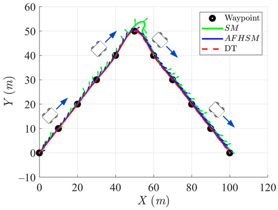
Figure 3.
Trajectory-tracking and heading performance of the controlled AMR using SM and AFHSM control methods in scenario 1.

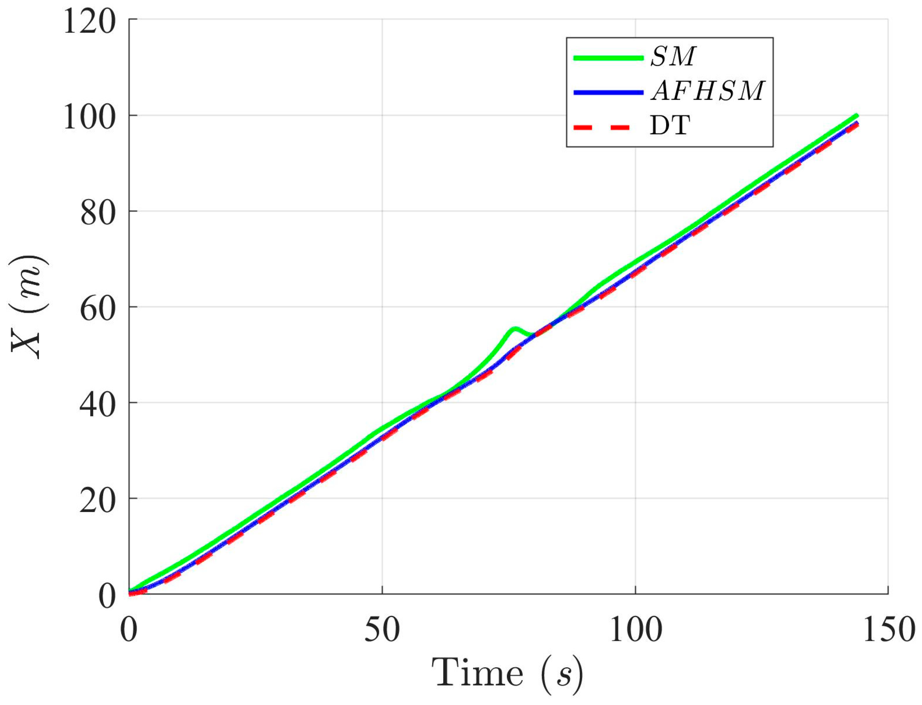
Figure 4.
Trajectory-tracking performance of the DT along the X-axis with SM and AFHSM control methods in scenario 1.
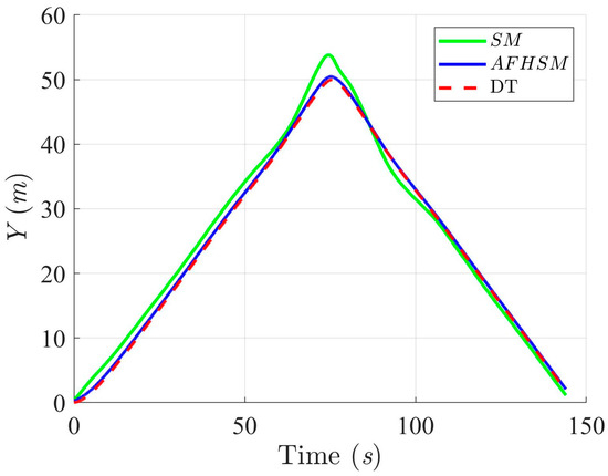
Figure 5.
Trajectory-tracking performance of the DT along the Y-axis with SM and AFHSM control methods in scenario 1.

Figure 6.
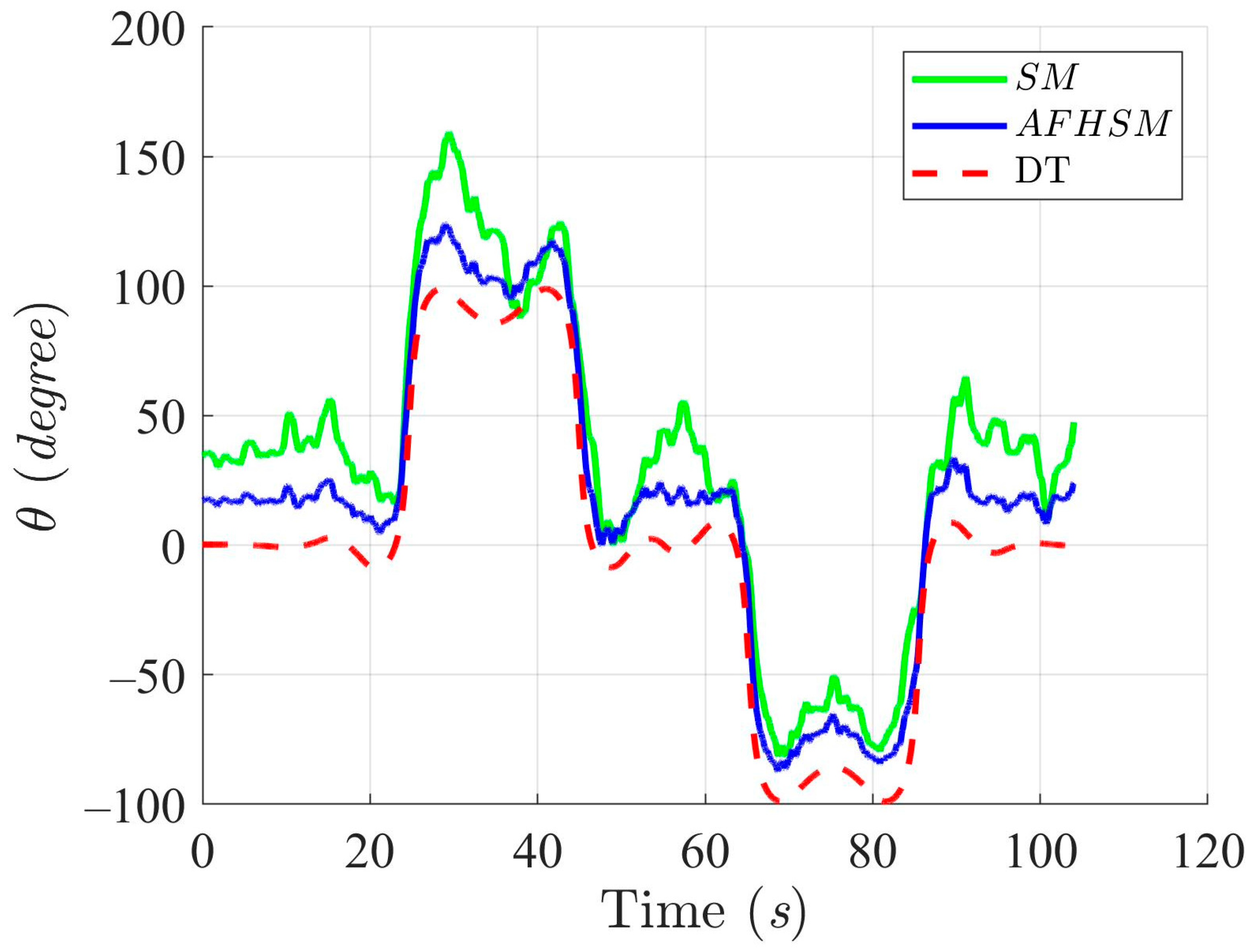
Trajectory-tracking performance of the DT at an angle, , with SM and AFHSM control methods in Scenario 1.
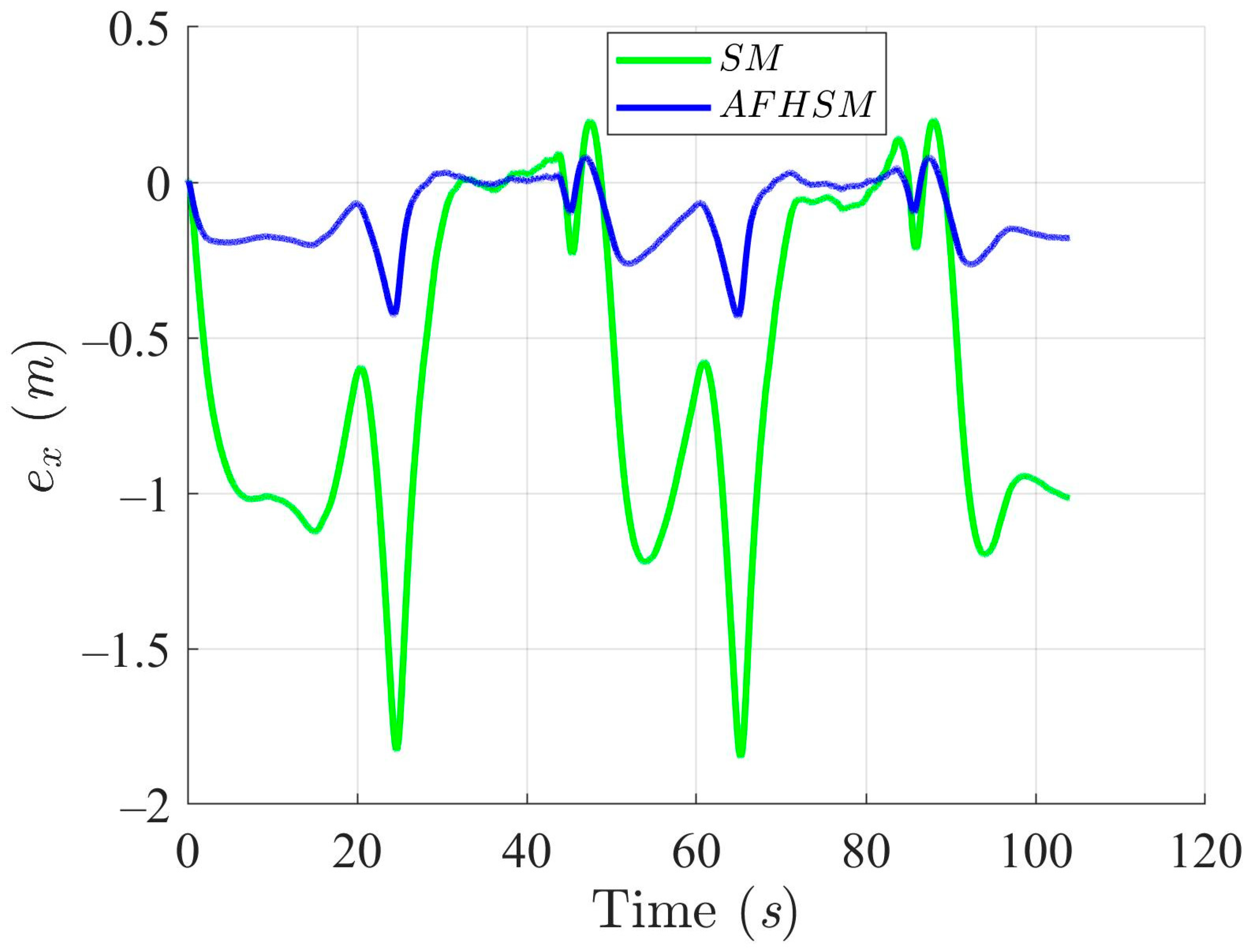
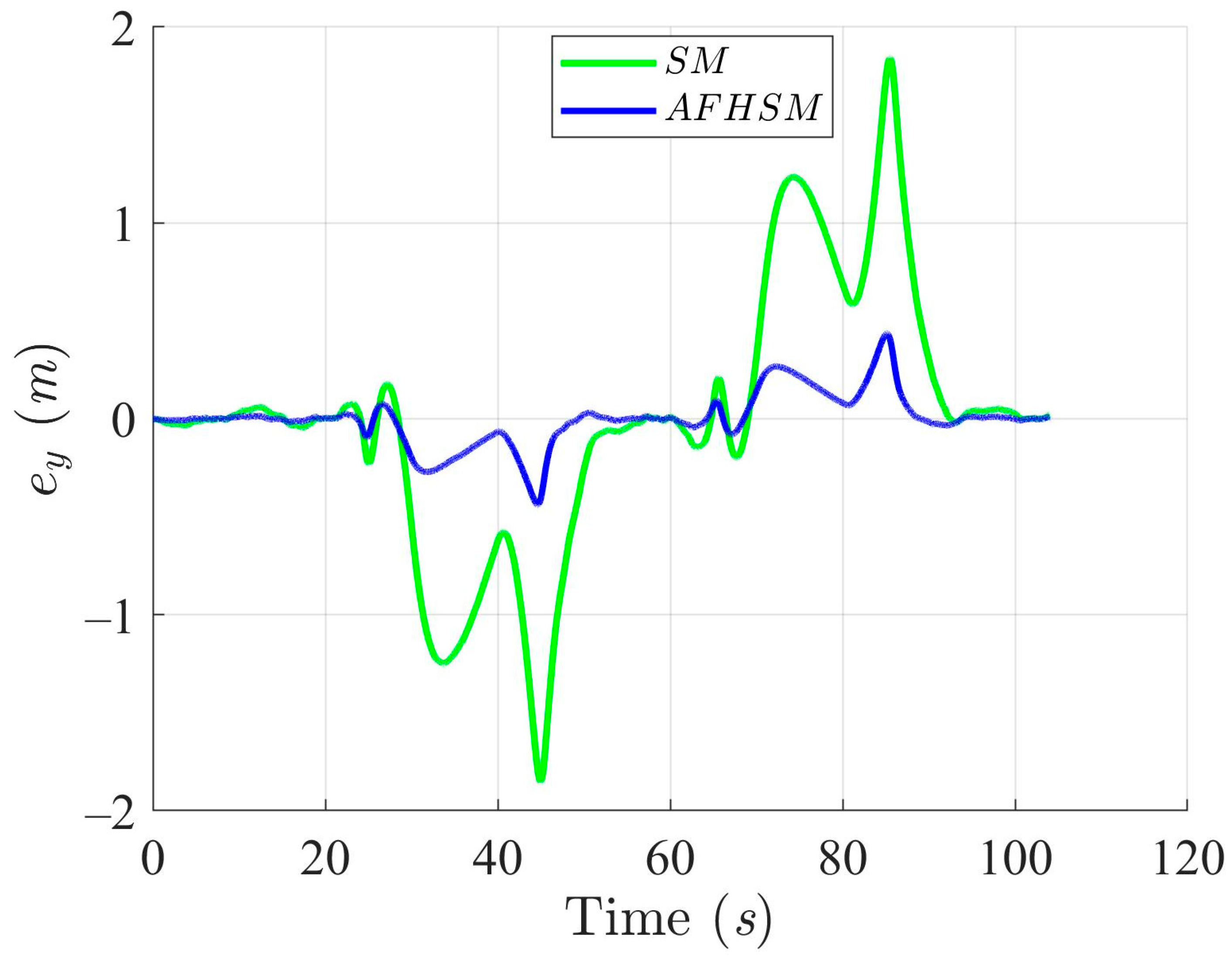
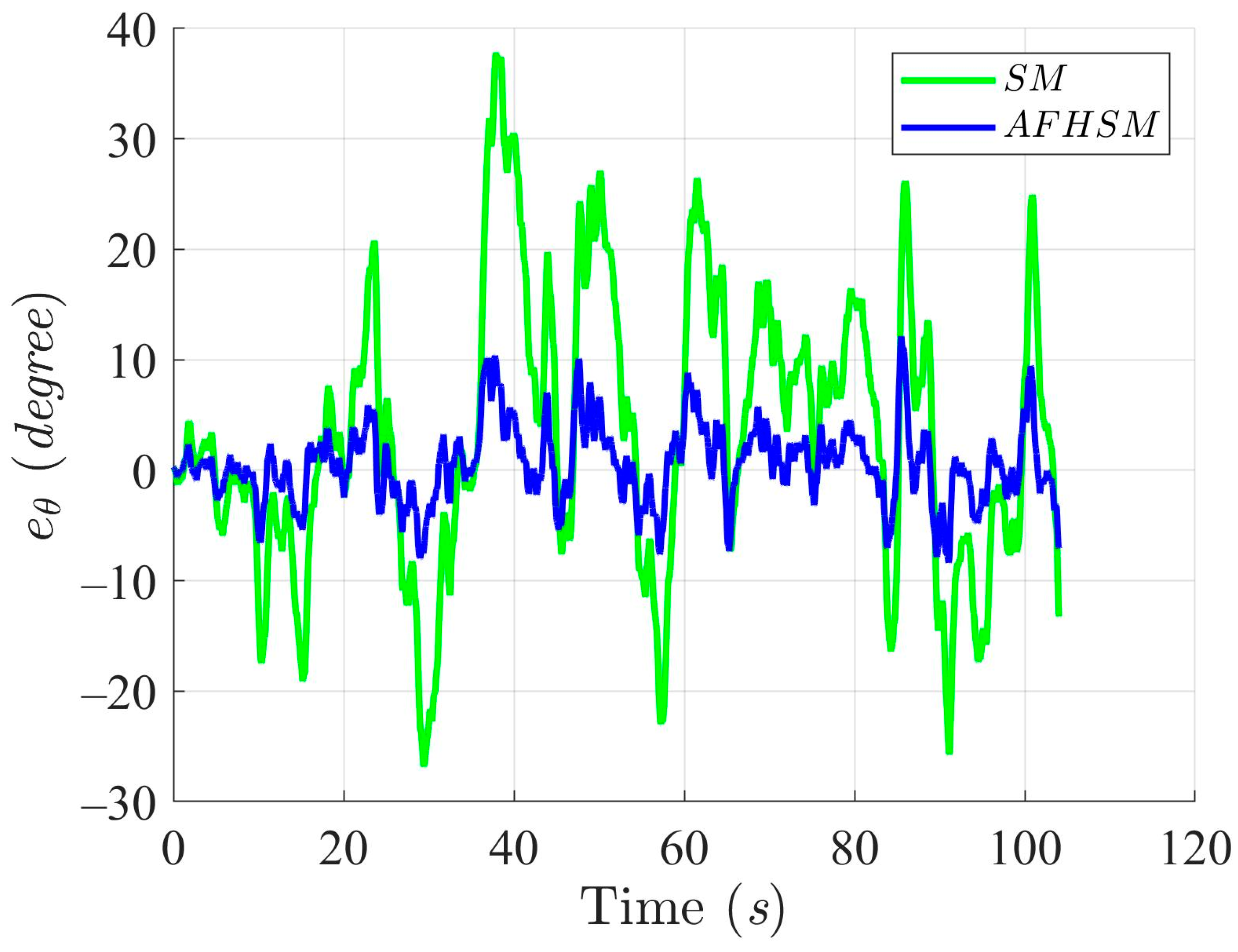
Figure 7, Figure 8 and Figure 9 provide detailed insights into the tracking error in the XY plane and the corresponding heading angle deviation for both methods. Under 60% uncertainty, the SM controller exhibited substantial deviations from the desired path, particularly around turning points, where rapid changes in direction exacerbate heading instability. These fluctuations not only increase trajectory-tracking errors but also reveal a fundamental limitation in the SM controller’s ability to handle nonlinear dynamics under high levels of uncertainty. In stark contrast, the AFHSM controller maintains tracking errors within a narrow bound and ensures stable heading regulation even during aggressive trajectory segments. This performance advantage is attributed to the adaptive fuzzy inference mechanism, which dynamically estimates and compensates for unknown disturbances and model uncertainties in real time.
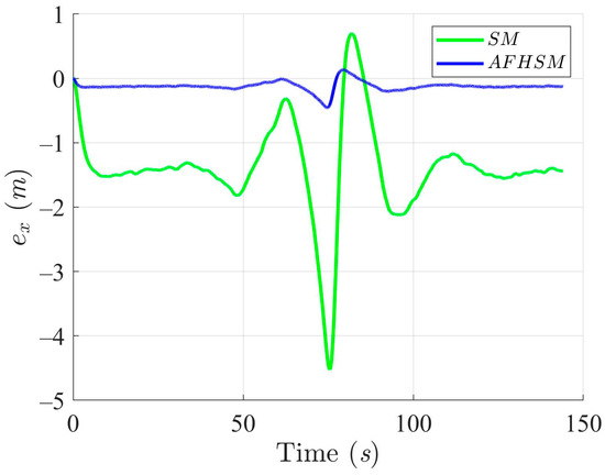
Figure 7.
X-axis trajectory-tracking errors using SM and AFHSM control methods in scenario 1.

Figure 8.
Y-axis trajectory-tracking errors using SM and AFHSM control methods in scenario 1.
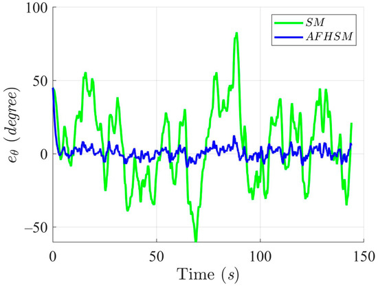
Figure 9.
Heading angle, , trajectory-tracking errors using SM and AFHSM control methods in scenario 1.
A closer inspection of Figure 3, Figure 6 and Figure 9 reveals that the SM-controlled AMR frequently overshoots or oscillates during trajectory correction, especially in segments with a sharp curvature. These behaviors are symptomatic of the limited adaptability and insufficient robustness of the SM control strategy. The AFHSM controller, however, demonstrates smooth trajectory adherence and superior pose convergence due to its hybrid architecture, which synergistically integrates the higher-order SM control with fuzzy logic and adaptive parameter tuning.
Furthermore, the control torques illustrated in Figure 10, Figure 11 and Figure 12 highlight another key benefit of the AFHSM method. Despite achieving higher tracking accuracy, the AFHSM controller consistently requires lower control torque magnitudes compared to the SM method. This observation underscores the energy efficiency of the AFHSM approach, as it reduces unnecessary control efforts while maintaining system stability. Such efficiency is particularly valuable in real-world AMR applications, where power consumption is a critical constraint.

Figure 10.
X-axis trajectory-tracking torques with SM and AFHSM control methods in scenario 1.
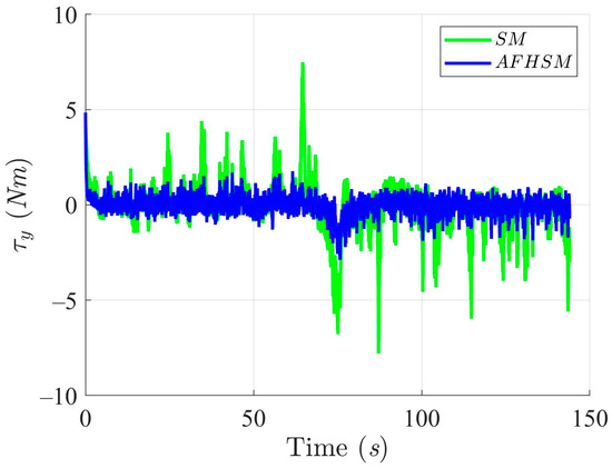
Figure 11.
Y-axis trajectory-tracking torques with SM and AFHSM control methods in scenario 1.

Figure 12.
Heading angle, , trajectory-tracking torques with SM and AFHSM control methods in scenario 1.
In summary, the simulation results for under 60% model uncertainty confirm the superior performance of the AFHSM controller over the conventional SM controller. The AFHSM method effectively minimizes tracking and heading errors, suppresses chattering effects, and delivers smooth control actions with reduced torque demands. These capabilities not only enhance trajectory stability and tracking precision but also contribute to the extended operational lifespan and reliability of autonomous systems. The results strongly support the AFHSM controller as a robust and energy-efficient solution for high-accuracy AMR navigation in uncertain and dynamically changing environments.
4.3.2. Scenario 2 (Convex-Shaped Trajectory)
In simulation scenario 2, a convex-shaped trajectory was generated by defining 21 waypoints, as shown in Table 5, which serves as the DT for this scenario. The design of this convex-shaped trajectory aims to challenge the performance of the control methods, as it combines straight-line motion with sharp directional changes. The trajectory primarily consists of five straight segments and four sharp turns, requiring high precision in trajectory tracking and the effective handling of sudden changes in direction. In particular, the sharp turns present a significant challenge for the control system, as they demand quick adjustments to the AMR’s heading while maintaining smooth and accurate trajectory tracking.
Table 5.
Predefined waypoints for the DT in scenario 2.
After establishing the convex-shaped trajectory, the SM and AFHSM control methods were implemented for trajectory tracking. These control strategies were chosen due to their ability to effectively manage the complexities introduced by sharp turns and the need for precise tracking. The simulation setup aimed to evaluate and compare the effectiveness of both methods in ensuring that the AMR tracks the DT with minimal errors and disturbances. The focus of this comparison is on how each control method manages the transition between straight segments and sharp turns while maintaining stability and minimizing tracking errors. This scenario is designed to highlight the strengths and limitations of both control methods in performing trajectory-tracking tasks under dynamic, realistic conditions, particularly in the presence of model uncertainties and external disturbances. The initial conditions of the controlled AMR used in scenario 2 are provided in Table 6.
Table 6.
Initial conditions of controlled AMR for scenario 2.
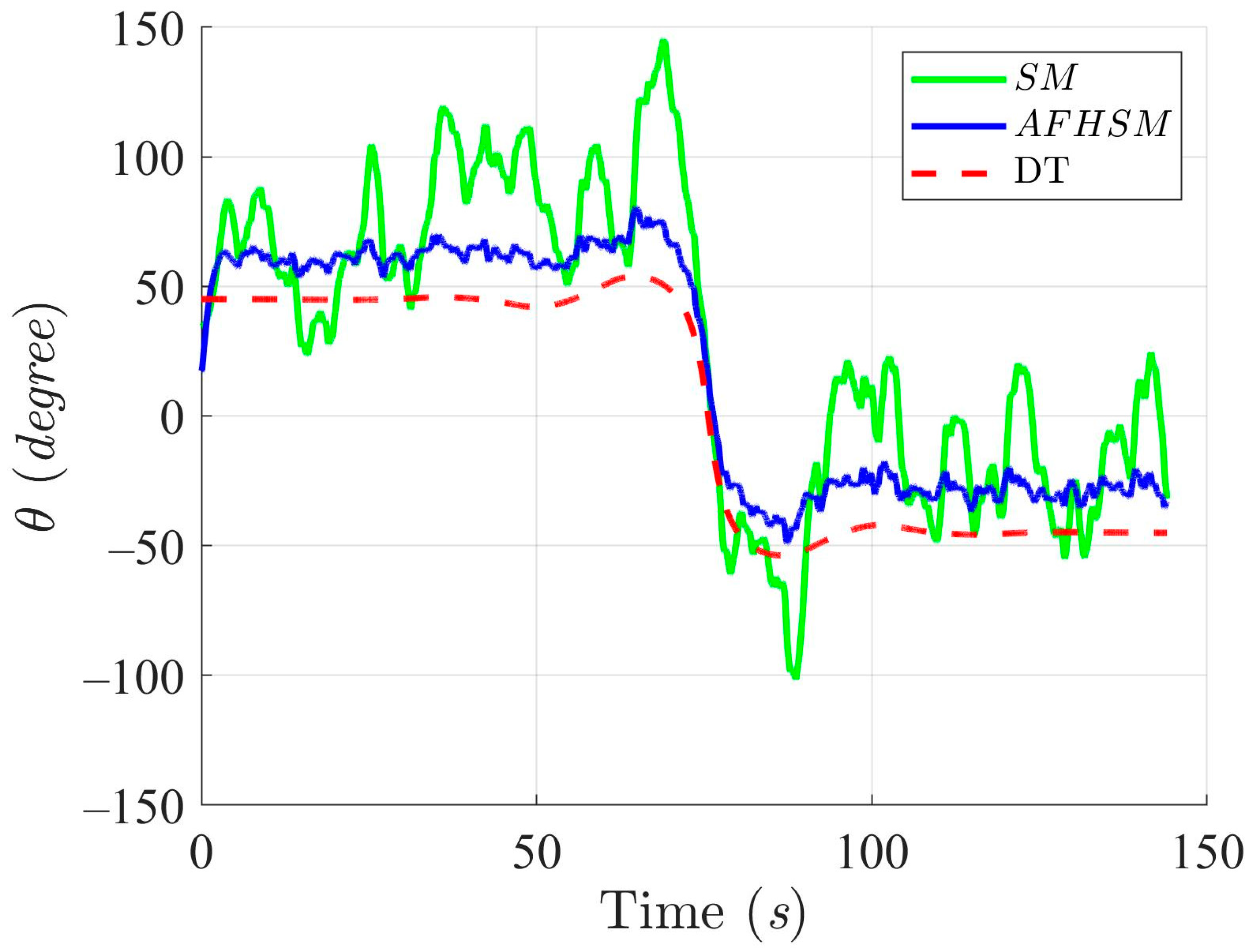
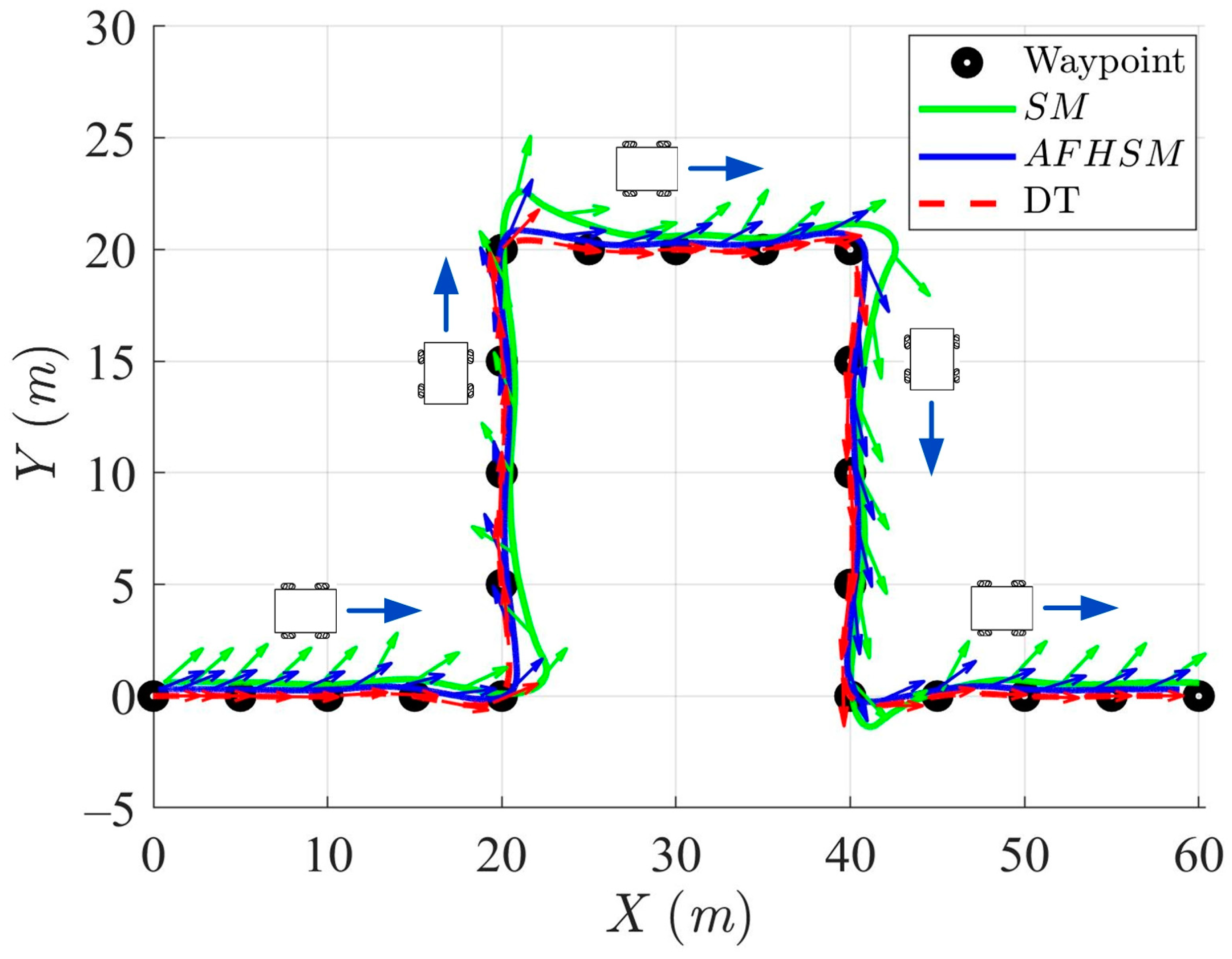
Figure 13, Figure 14, Figure 15 and Figure 16 illustrate the trajectory and pose tracking performance of the AMR as it follows DT under a validation scenario involving up to 60% model uncertainty. This simulation setting is intentionally designed to assess controller robustness under moderate yet significant deviations from the nominal model. The performance of the two control strategies was compared: conventional SM control and proposed AFHSM control.
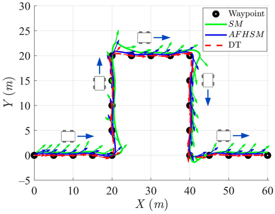
Figure 13.
Trajectory-tracking and heading performance of the controlled AMR using SM and AFHSM control methods in scenario 2.

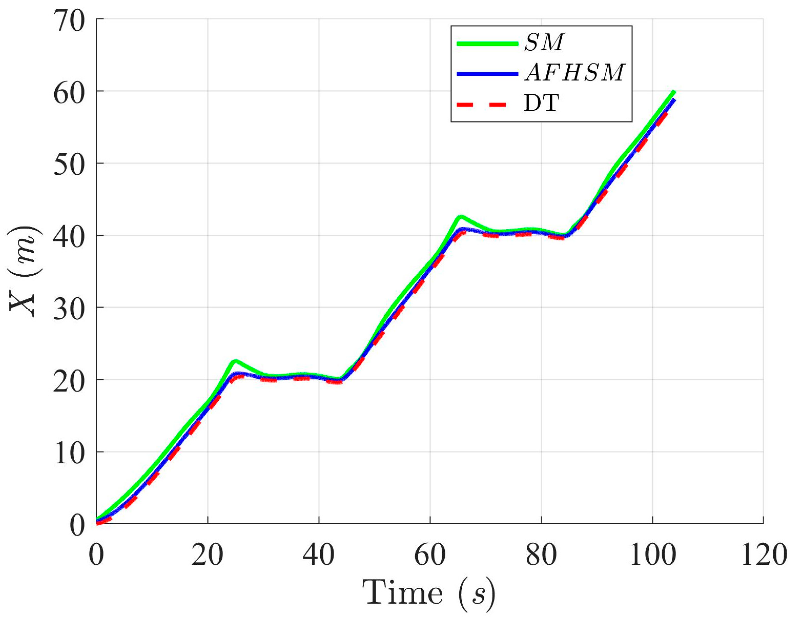
Figure 14.
Trajectory-tracking performance of the DT along the X-axis with SM and AFHSM control methods in scenario 2.

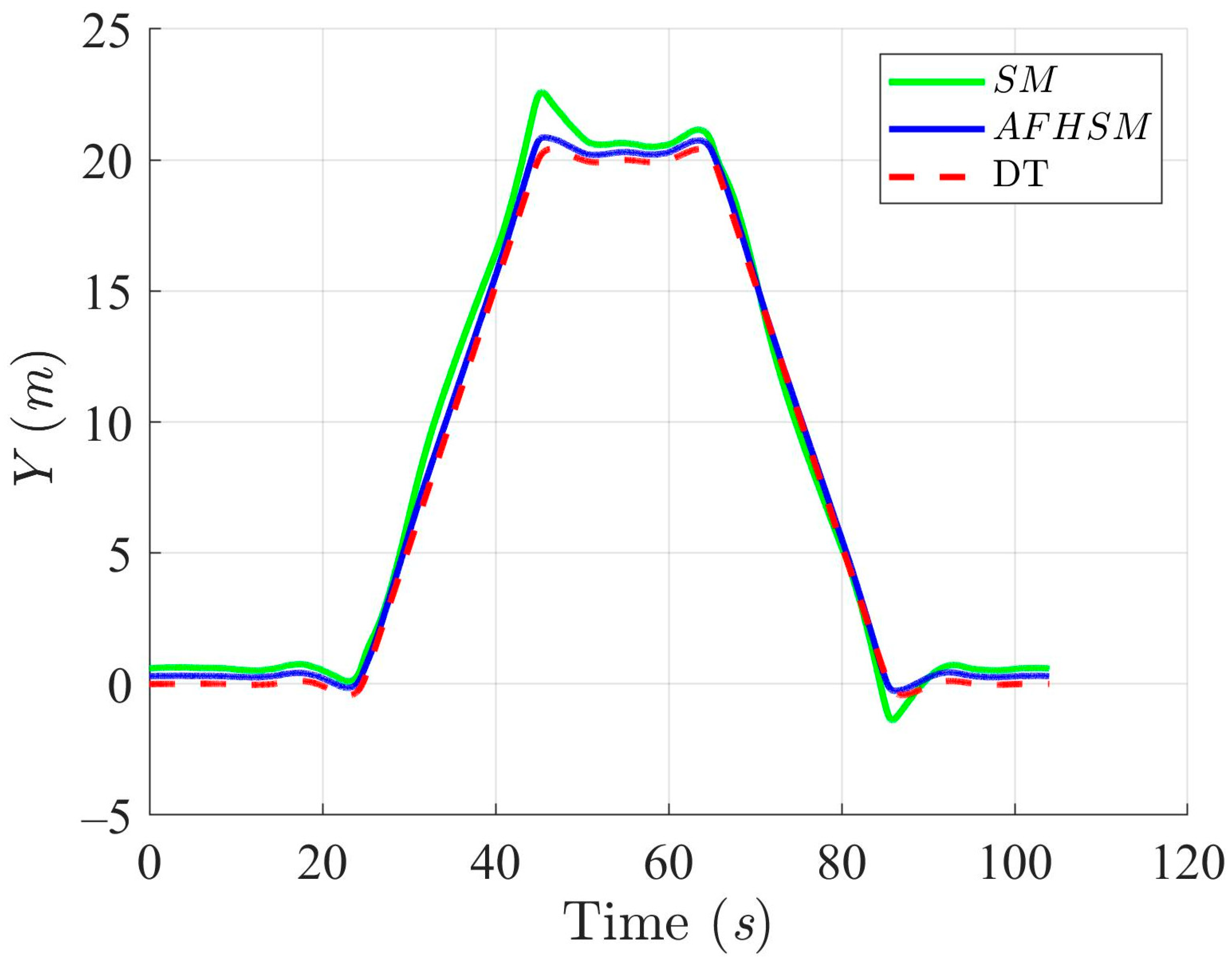
Figure 15.
Trajectory-tracking performance of the DT along the Y-axis with SM and AFHSM control methods in scenario 2.

Figure 16.
Trajectory-tracking performance of the DT at an angle, , with SM and AFHSM control methods in Scenario 2.
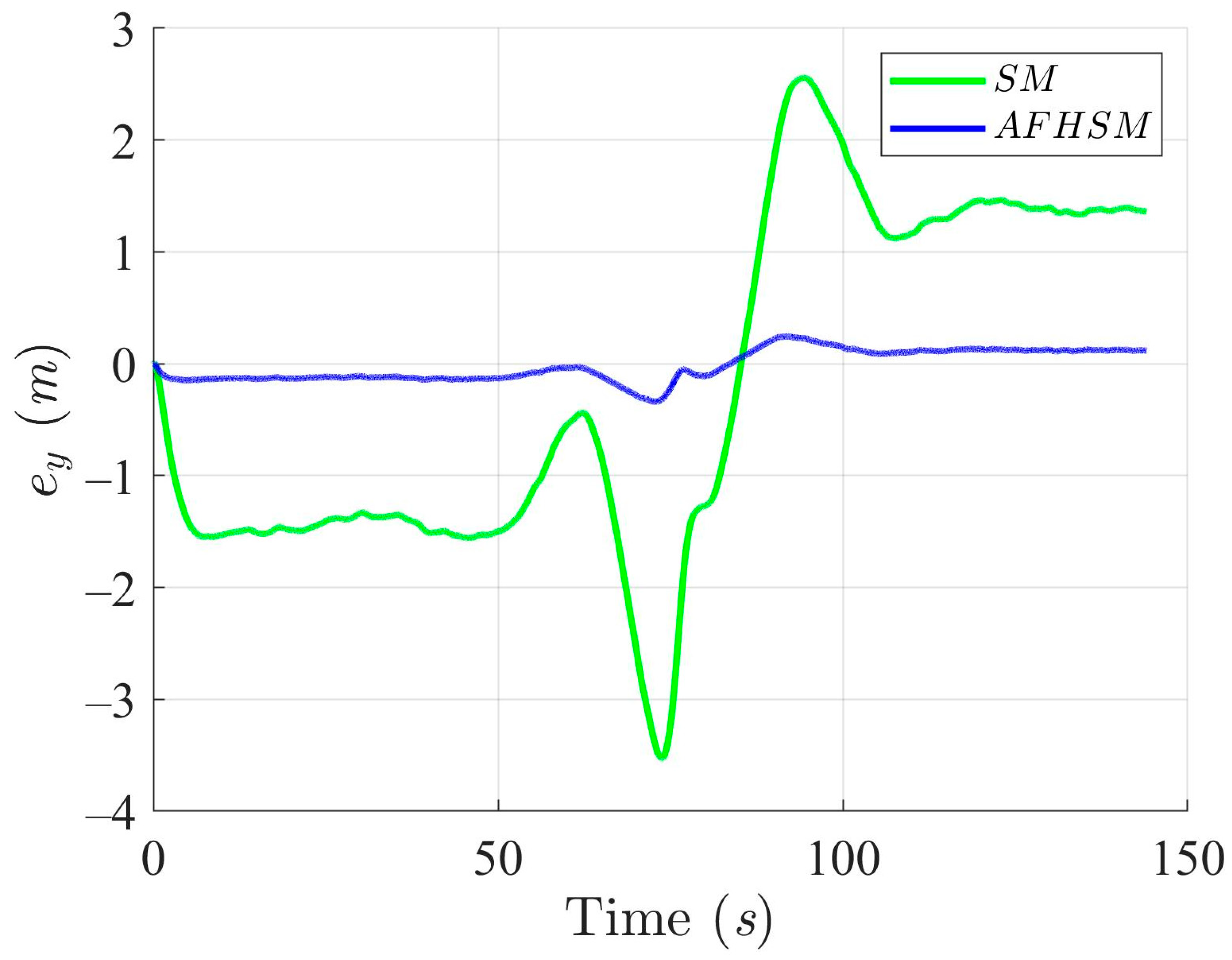
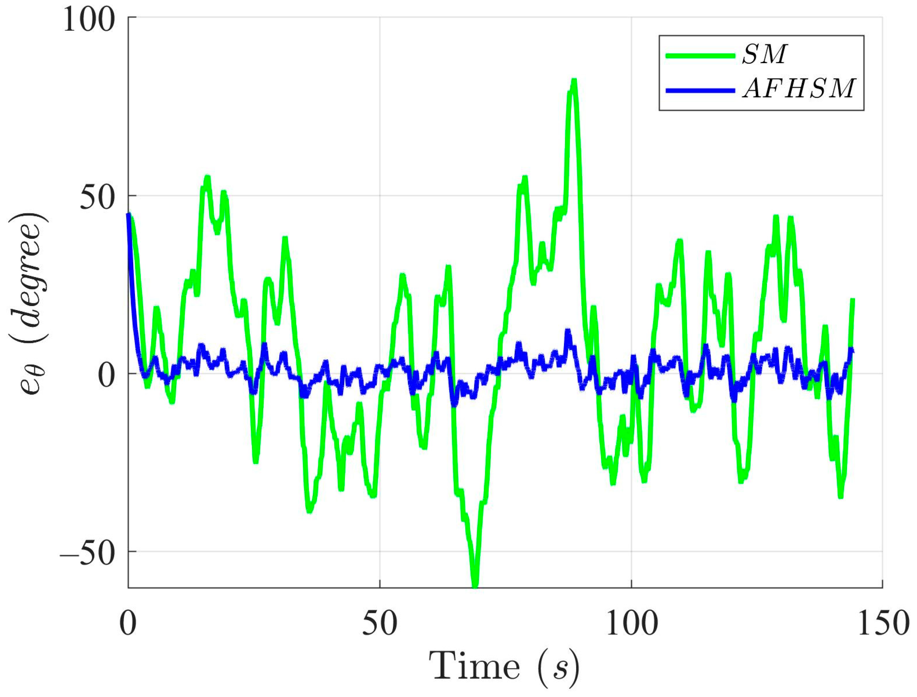
Figure 17, Figure 18 and Figure 19 further depict the tracking errors in the XY plane along with the corresponding heading angle errors. While the level of model uncertainty was relatively moderate compared to more extreme test cases, the SM control method still exhibited noticeable tracking and orientation deviations, particularly at turning points. These errors reflect the limited adaptability of the SM controller in dealing with structural discrepancies in the system dynamics, even when uncertainty is constrained to 60%.

Figure 17.
X-axis trajectory-tracking errors using SM and AFHSM control methods in scenario 2.

Figure 18.
Y-axis trajectory-tracking errors using SM and AFHSM control methods in scenario 2.
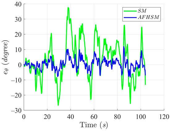
Figure 19.
Heading angle, , trajectory-tracking errors using SM and AFHSM control methods in scenario 2.
In contrast, the AFHSM control method demonstrates superior performance, consistently achieving lower tracking and heading angle errors. This robustness is attributed to the controller’s ability to dynamically compensate for parametric uncertainties through the integration of adaptive fuzzy inference and high-order SM techniques. A detailed inspection of Figure 13, Figure 16 and Figure 19 highlights the AFHSM controller’s effectiveness in maintaining smooth trajectory adherence and heading stability, whereas the SM-controlled AMR experiences transient oscillations during directional transitions.
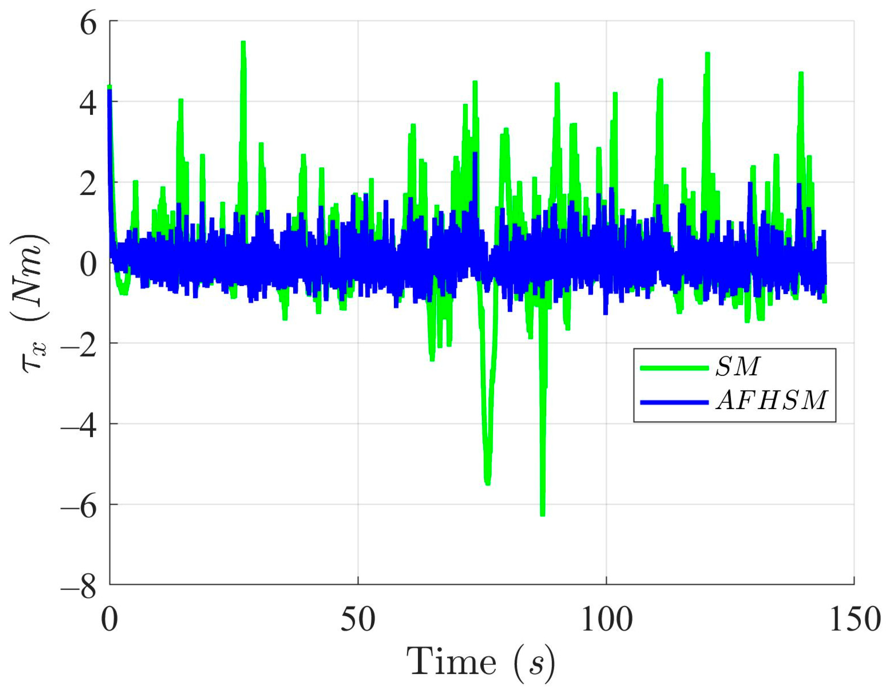
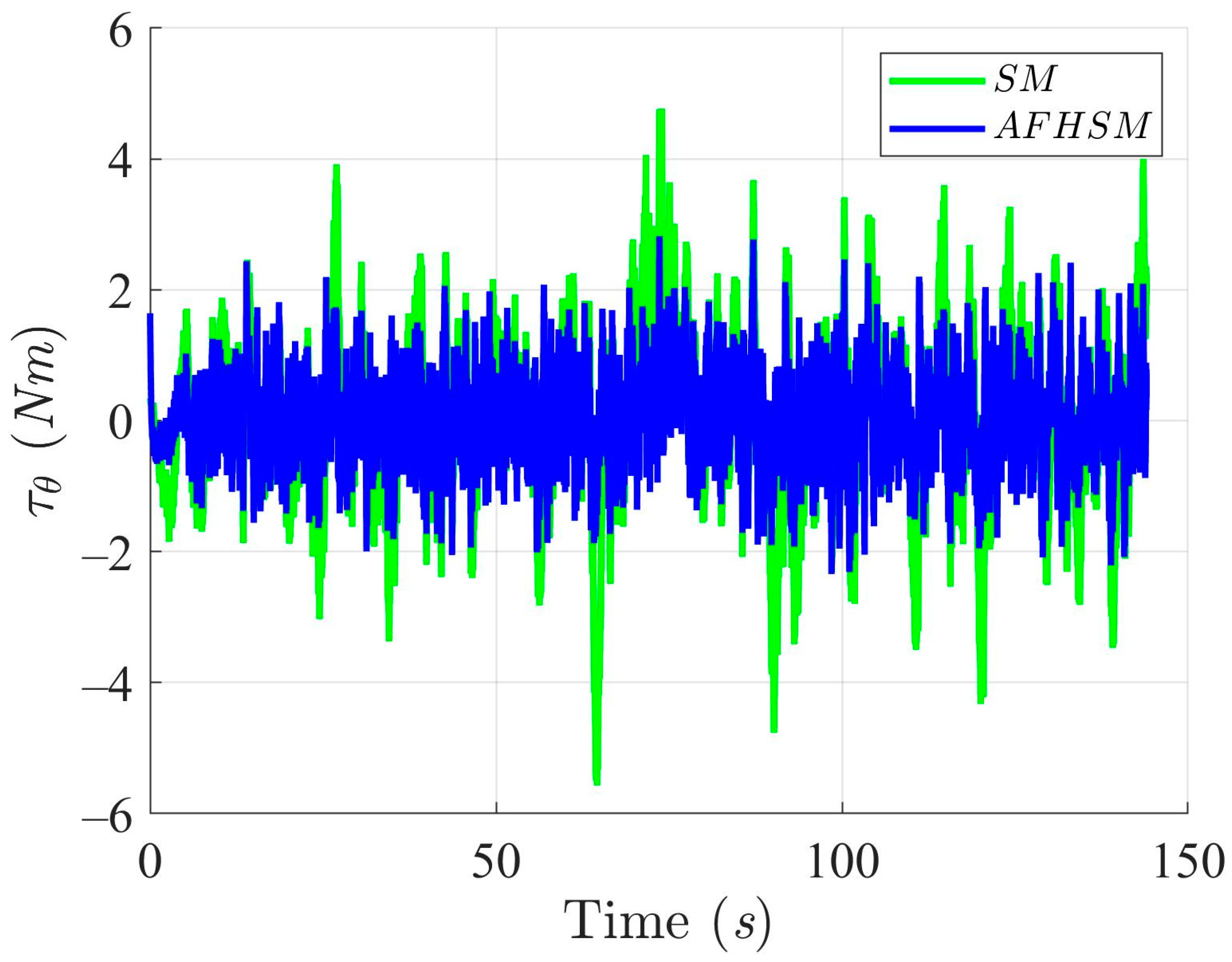
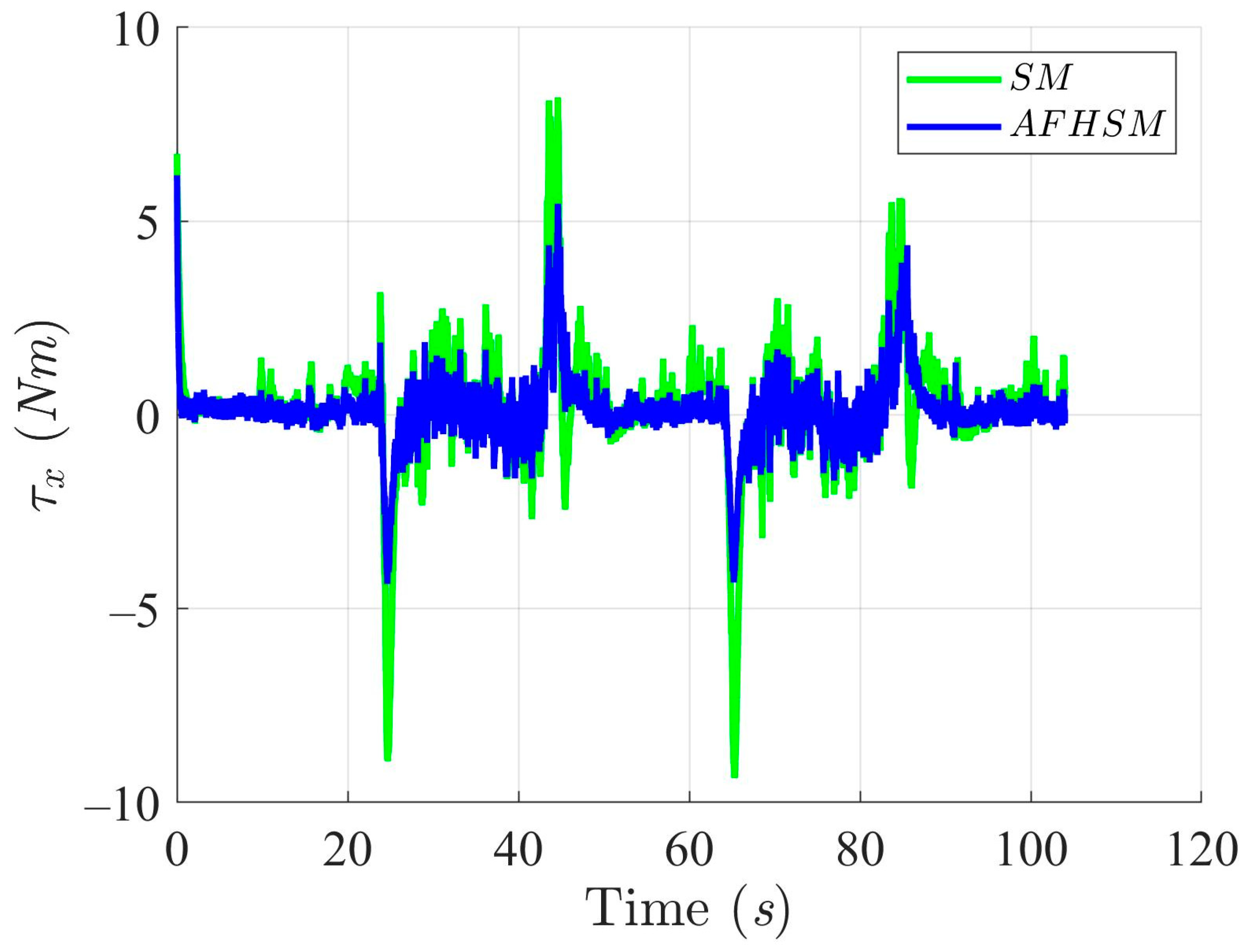
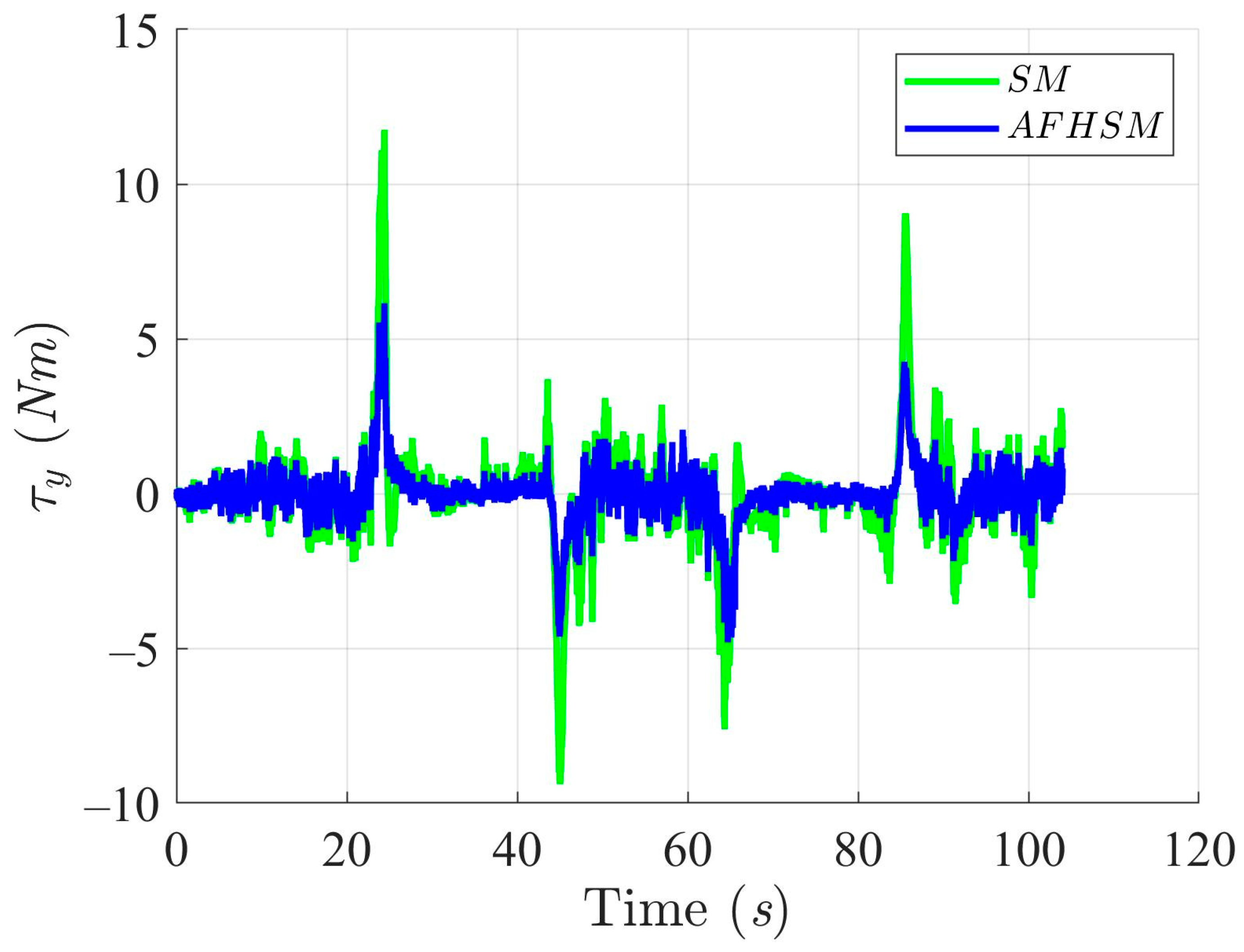
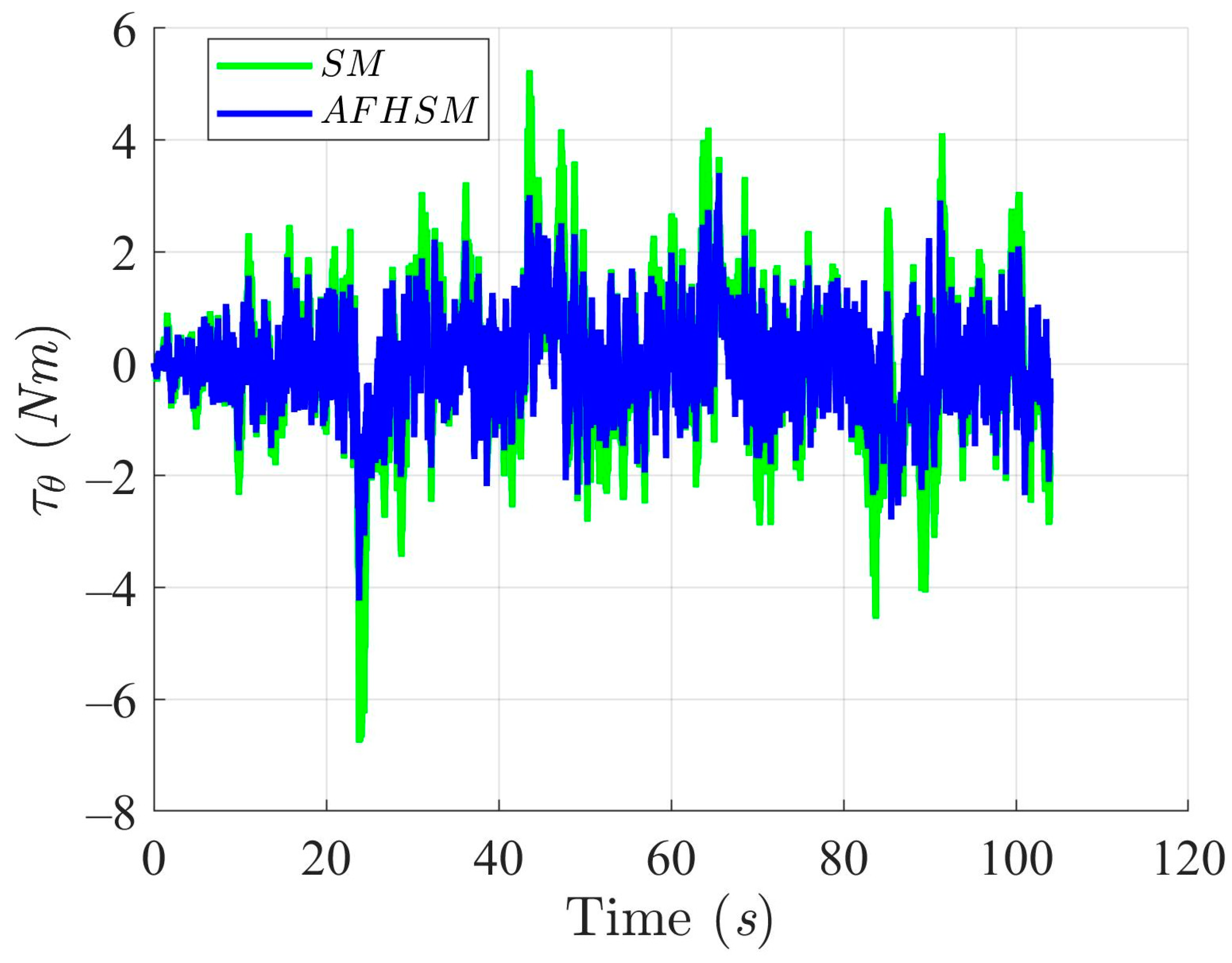
Moreover, Figure 20, Figure 21 and Figure 22 show the control torques applied by both methods. The AFHSM controller produces smoother and more energy-efficient torque profiles, indicating not only improved tracking precision but also a reduced actuator workload. This aspect is critical for AMR platforms where energy efficiency directly influences mission duration and system reliability.

Figure 20.
X-axis trajectory-tracking torques with SM and AFHSM control methods in scenario 2.

Figure 21.
Y-axis trajectory-tracking torques with SM and AFHSM control methods in scenario 2.
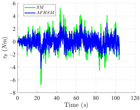
Figure 22.
Heading angle, , trajectory-tracking torques with SM and AFHSM control methods in scenario 2.
In summary, the simulation results conducted under 60% model uncertainty confirm the superior robustness and effectiveness of the AFHSM control method over classical SM control. The AFHSM controller achieves precise trajectory tracking, minimizes heading fluctuations, and optimally regulates control inputs. These capabilities make it a compelling solution for real-world AMR applications where high-accuracy navigation is required under uncertain and dynamically changing conditions.
5. Conclusions
This study presents a nonlinear AFHSM control method specifically designed to address the trajectory-tracking problem of AMRs under model uncertainties and external disturbances. The proposed control method effectively combines the strong robustness of SM control with the high flexibility of adaptive fuzzy logic, significantly improving the tracking accuracy and stability of the AMR system in complex environments. Furthermore, the method demonstrates the robustness of the AMR trajectory-tracking system, ensuring stable operation despite various model uncertainties and external disturbances, highlighting its superior disturbance rejection capabilities. To further validate the performance of the proposed control method, a Lyapunov analysis was conducted, rigorously establishing the stability of the nonlinear closed-loop system. This analysis not only guarantees the mathematical feasibility of the system but also provides a solid theoretical foundation for practical applications. To comprehensively assess the effectiveness of the AFHSM control method, two comparative simulations were performed against the SM control method, using triangle-shaped and convex-shaped trajectories as the DTs for AMR trajectory tracking. The simulation results, with a model uncertainty of 60%, show that the AFHSM control method significantly outperforms the SM control method, exhibiting clear advantages in the control response speed, trajectory-tracking accuracy, and adaptability to model uncertainties and external disturbances.
Although the proposed AFHSM control method demonstrates strong robustness and superior trajectory-tracking performance under uncertainty, several avenues for future research remain. First, experimental validation on a physical AMR platform equipped with Mecanum wheels is essential to further verify the controller’s real-time effectiveness and robustness in dynamic, real-world environments. Second, extending the control strategy to account for time-delay effects, sensor noise, or actuator constraints would enhance its practical applicability. Third, the integration of learning-based techniques, such as reinforcement learning or neural networks, could be explored to further improve adaptation speed and reduce reliance on predefined fuzzy rules. Additionally, future studies may consider multi-robot coordination under the proposed control framework to enable cooperative trajectory tracking in swarm or fleet robotics scenarios. Finally, the optimization of the control law with respect to energy efficiency and computational cost would facilitate deployment on resource-constrained embedded systems.
Funding
This research received no external funding.
Data Availability Statement
All data revealed in this paper were generated during the study.
Conflicts of Interest
The author declares no conflicts of interest.
References
- Xiao, H.; Li, Z.; Yang, C.; Zhang, L.; Yuan, P.; Ding, L.; Wang, T. Robust Stabilization of a Wheeled Mobile Robot Using Model Predictive Control Based on Neuro Dynamics Optimization. IEEE Trans. Ind. Electron. 2017, 64, 505–516. [Google Scholar] [CrossRef]
- Zhang, Y.; Zhao, X.; Tao, B.; Ding, H. Point Stabilization of Nonholonomic Mobile Robot by Bézier Smooth Subline Constraint Nonlinear Model Predictive Control. IEEE/ASME Trans. Mechatron. 2021, 26, 990–1001. [Google Scholar] [CrossRef]
- Abbasi, A.; Moshayedi, A.J. Trajectory Tracking of Two-wheeled Mobile Robots, Using LQR Optimal Control Method, Based on Computational Model of KHEPERA IV. J. Simul. Anal. Novel Technol. Mech. Eng. 2018, 10, 41–50. [Google Scholar]
- Abut, T.; Huseyn, M. Modeling and Optimal Trajectory Tracking Control of Wheeled a Mobile Robot. Cauc. J. Sci. 2019, 6, 137–146. [Google Scholar]
- Rossomando, F.G. Adaptive Neural Dynamic Compensator for Mobile Robots in Trajectory Tracking Control. IEEE Lat. Am. Trans. 2011, 9, 593–602. [Google Scholar] [CrossRef]
- Bamgbose, S.O.; Qian, X.L.L. Trajectory Tracking Control Optimization with Neural Network for Autonomous Vehicles. Adv. Sci. Technol. Eng. Syst. J. 2019, 4, 217–224. [Google Scholar] [CrossRef]
- Najva, H.; Abdul, S. Neural Network Based Adaptive Controller for Trajectory Tracking of Wheeled Mobile Robots. IEEE Access 2022, 10, 13582–13597. [Google Scholar]
- Trinh, T.K.L.; Nguyen, T.T.; Hoang, T.; Thai, N. A Neural Network Controller Design for the Mecanum Wheel Mobile Robot. Eng. Technol. Appl. Sci. Res. 2023, 13, 10541–10547. [Google Scholar]
- Peng, S.; Shi, W. Adaptive Fuzzy Output Feedback Control of a Nonholonomic Wheeled Mobile Robot. IEEE Access 2018, 6, 43414–43424. [Google Scholar] [CrossRef]
- Kong, L.; He, W.; Yang, C.; Li, Z.; Sun, C. Adaptive Fuzzy Control for Coordinated Multiple Robots with Constraint Using Impedance Learning. IEEE Trans. Cybern. 2019, 49, 3052–3063. [Google Scholar] [CrossRef]
- Abougarair, A.J. Model Reference Adaptive Control and Fuzzy Optimal Controller for Mobile Robot. J. Multidiscip. Eng. Sci. Technol. 2019, 6, 9722–9728. [Google Scholar]
- Zhang, P.; Zhang, J.; Zhang, Z. Design of RBFNN-based Adaptive Sliding Mode Control Strategy for Active Rehabilitation Robot. IEEE Access 2020, 8, 155538–155547. [Google Scholar] [CrossRef]
- Shi, H.; Xu, M.; Hwang, K. A Fuzzy Adaptive Approach to Decoupled Visual Servoing for a Wheeled Mobile Robot. IEEE Trans. Fuzzy Syst. 2020, 28, 3229–3243. [Google Scholar] [CrossRef]
- Chen, Y.-H.; Chen, Y.-Y. Nonlinear Adaptive Fuzzy Control Design for Wheeled Mobile Robots Using the Skew Symmetrical Property. Symmetry 2023, 15, 221. [Google Scholar] [CrossRef]
- Zhai, J.-Y.; Song, Z.-B. Adaptive Sliding Mode Trajectory Tracking Control for Wheeled Mobile Robots. Int. J. Control 2019, 92, 2255–2262. [Google Scholar] [CrossRef]
- Wang, G.; Zhou, C.; Yu, Y.; Liu, X. Adaptive Sliding Mode Trajectory Tracking Control for WMR Considering Skidding and Slipping via Extended State Observer. Energies 2019, 12, 3305. [Google Scholar] [CrossRef]
- Mustafa, A.; Dhar, N.K.; Verma, N.K. Event-triggered Sliding Mode Control for Trajectory Tracking of Nonlinear Systems. IEEE/CAA J. Autom. Sin. 2020, 7, 307–314. [Google Scholar] [CrossRef]
- Liu, K.; Gao, H.; Ji, H.; Hao, Z. Adaptive Sliding Mode Based Disturbance Attenuation Tracking Control for Wheeled Mobile Robots. Int. J. Contr. Autom. Syst. 2020, 18, 1288–1298. [Google Scholar] [CrossRef]
- Zhang, H.; Li, B.; Xiao, B.; Yang, Y.; Ling, J. Nonsingular Recursive-structure Sliding Mode Control for High-order Nonlinear Systems and an Application in a Wheeled Mobile Robot. ISA Trans. 2020, 130, 553–564. [Google Scholar] [CrossRef]
- Li, B.; Zhang, H.; Xiao, B.; Wang, C.; Yang, Y. Fixed-time Integral Sliding Mode Control of a High-order Nonlinear System. Nonlinear Dyn. 2022, 107, 909–920. [Google Scholar] [CrossRef]
- Zheng, Y.; Zheng, J.; Shao, K.; Zhao, H.; Xie, H.; Wang, H. Adaptive Trajectory Tracking Control for Nonholonomic Wheeled Mobile Robots: A Barrier Function Sliding Mode Approach. IEEE/CAA J. Autom. Sin. 2024, 11, 1007–1021. [Google Scholar] [CrossRef]
- Abadi, A.; Ayeb, A.; Labbadi, M.; Fofi, D.; Bakir, T.; Mekki, H. Robust Tracking Control of Wheeled Mobile Robot Based on Differential Flatness and Sliding Active Disturbance Rejection Control: Simulations and Experiments. Sensors 2024, 24, 2849. [Google Scholar] [CrossRef] [PubMed]
- Tiep, D.K.; Lee, K.; Im, D.-Y.; Kwak, B.; Ryoo, Y.-J. Design of Fuzzy-PID Controller for Path Tracking of Mobile Robot with Differential Drive. Int. J. Fuzzy Log. Intell. Syst. 2018, 18, 220–228. [Google Scholar] [CrossRef]
- Xiong, R.; Li, L.; Zhang, C.; Ma, K.; Yi, X.; Zeng, H. Path Tracking of a Four-Wheel Independently Driven Skid Steer Robotic Vehicle Through a Cascaded NTSM-PID Control Method. IEEE Trans. Instrum. Meas. 2022, 71, 1–11. [Google Scholar] [CrossRef]
- Khan, H.; Khatoon, S.; Gaur, P.; Abbas, M.; Saleel, C.A.; Khan, S.A. Speed Control of Wheeled Mobile Robot by Nature-Inspired Social Spider Algorithm-Based PID Controller. Processes 2023, 11, 1202. [Google Scholar] [CrossRef]
- Rasha, M.H. Design a New Hybrid Controller Based on an Improvement Version of Grey Wolf Optimization for Trajectory Tracking of Wheeled Mobile Robot. FME. Trans. 2023, 51, 140–148. [Google Scholar]
- Muhamad, A.; Riky, D.P. Mecanum 4 Omni Wheel Directional Robot Design System Using PID Method. J. Fuzzy Syst. Control 2023, 1, 6–13. [Google Scholar]
- Wu, X.; Jin, P.; Zou, T.; Qi, Z.; Xiao, H.; Lou, P. Backstepping Trajectory Tracking Based on Fuzzy Sliding Mode Control for Differential Mobile Robots. J. Intell. Robot. Syst. 2019, 96, 109–121. [Google Scholar] [CrossRef]
- Fadlo, S.; Elmahjoub, A.A.; Rabbah, N. Optimal Trajectory Tracking Control for a Wheeled Mobile Robot Using Backstepping Technique. Int. J. Electr. Comput. Eng. 2022, 12, 5979–5987. [Google Scholar] [CrossRef]
- Jiang, M.; Chen, L.; Wang, Y.; Wu, H. Adaptive Backstepping Control for Mecanum-Wheeled Omnidirectional Vehicle Using Neural Networks. IEEJ Trans. Electr. Electron. Eng. 2022, 17, 378–386. [Google Scholar] [CrossRef]
- He, N.; Yang, Z.; Fan, X.; Wu, J.; Sui, Y.; Zhang, Q. A Self-Adaptive Double Q-Backstepping Trajectory Tracking Control Approach Based on Reinforcement Learning for Mobile Robots. Actuators 2023, 12, 326. [Google Scholar] [CrossRef]
- Chai, B.; Zhang, K.; Tan, M. An Optimal Robust Trajectory Tracking Control Strategy for the Wheeled Mobile Robot. Int. J. Control Autom. Syst. 2024, 22, 1050–1065. [Google Scholar] [CrossRef]
- Xie, H.; Zheng, J.; Sun, Z.; Wang, H.; Chai, R. Finite-time Tracking Control for Nonholonomic Wheeled Mobile Robot Using Adaptive Fast Nonsingular Terminal Sliding Mode. Nonlinear Dyn. 2022, 110, 1437–1453. [Google Scholar] [CrossRef]
- AmirReza, H.M.; Mohammad, M.F.; Seyed, M.A. A Finite-time Adaptive Taylor Series Tracking Control of Electrically-driven Wheeled Mobile Robots. IET Control Theory Appl. 2022, 16, 1042–1061. [Google Scholar]
- Roger, M.-C. Observer-based Finite-time Control for Trajectory Tracking of Wheeled Mobile Robots with Kinematic Disturbances. ISA Trans. 2024, 148, 64–77. [Google Scholar]
- Huang, J.; Chen, H.; Shen, C. Event-Triggered Model-Free Adaptive Control for Wheeled Mobile Robot with Time Delay and External Disturbance Based on Discrete-Time Extended State Observer. J. Dyn. Syst. Meas. Control 2023, 146, 021005. [Google Scholar] [CrossRef]
- Zhang, C.; Cen, C.; Huang, J. An Overview of Model-Free Adaptive Control for the Wheeled Mobile Robot. World Electr. Veh. J. 2024, 15, 396. [Google Scholar] [CrossRef]
- Duc, C.N.; Pham, S.H.T.; Vu, N.T.T. Model-Free Q-Learning-Based Adaptive Optimal Control for Wheeled Mobile Robot. J. Control Autom. Electr. Syst. 2025, 36, 86–100. [Google Scholar] [CrossRef]
- Petrov, P.; Kralov, I. Exponential Trajectory Tracking Control of Nonholonomic Wheeled Mobile Robots. Mathematics 2025, 13, 1. [Google Scholar] [CrossRef]
- Matthew, T.W.; Daniel, T.G.; Tony, J.P. Collinear Mecanum Drive: Modeling, Analysis, Partial Feedback Linearization, and Nonlinear Control. IEEE Trans. Robot. 2021, 37, 642–658. [Google Scholar]
- Carlos, M.-M.; Javier, P.-J.; Adrian, A.-D.; César, C.-H. Velocity and Position Tracking Controllers for Wheeled Mobile Robots. IFAC-Pap. OnLine 2023, 56, 2158–2163. [Google Scholar]
- Chen, Y.-H. Control Design and Implementation of Autonomous Robotic Lawnmower. Mathematics 2024, 12, 3324. [Google Scholar] [CrossRef]
- Chen, Y.-H.; Li, T.H.S.; Chen, Y.-Y. A Novel Nonlinear Control Law with Trajectory Tracking Capability for Mobile Robots: Closed-Form Solution Design. Appl. Math. Inf. Sci. 2013, 7, 749–754. [Google Scholar] [CrossRef]
- Chen, Y.-H.; Lou, S.-J. Control Design of a Swarm of Intelligent Robots: A Closed-Form H2 Nonlinear Control Approach. Appl. Sci. 2020, 10, 1055. [Google Scholar] [CrossRef]
- Chen, Y.-H.; Chen, Y.-Y. Trajectory Tracking Design for A Swarm of Autonomous Mobile Robots: A Nonlinear Adaptive Optimal Approach. Mathematics 2022, 10, 3901. [Google Scholar] [CrossRef]
- Chen, Y.-H. Nonlinear Adaptive Optimal Control Design and Implementation for Trajectory Tracking of Four-Wheeled Mecanum Mobile Robots. Mathematics 2024, 12, 4013. [Google Scholar] [CrossRef]
- Bounemeur, A.; Chemachema, M.; Zahaf, A.; Bououden, S. Adaptive Fuzzy Fault-Tolerant Control Using Nussbaum Gain for a Class of SISO Nonlinear Systems with Unknown Directions. In Proceedings of the 4th International Conference on Electrical Engineering and Control Applications, Constantine, Algeria, 17–19 December 2019. [Google Scholar]
- Bounemeur, A.; Chemachema, M. Adaptive Fuzzy Fault-Tolerant Control for a Class of Nonlinear Systems under Actuator Faults: Application to an Inverted Pendulum. Int. J. Robot. Cont. Syst. 2021, 1, 102–115. [Google Scholar] [CrossRef]
- Bounemeur, A.; Chemachema, M. Adaptive fuzzy fault-tolerant control using Nussbaum-type function with state-dependent actuator failures. Neural Comput. Appl. 2021, 33, 191–208. [Google Scholar] [CrossRef]
- Yan, S.; Gu, Z.; Park, J.H.; Xie, X. A Delay-Kernel-Dependent Approach to Saturated Control of Linear Systems with Mixed Delays. Automatica 2023, 152, 110984. [Google Scholar] [CrossRef]
- Yan, S.; Gu, Z.; Park, J.H.; Xie, X. Distributed-Delay-Dependent Stabilization for Networked Interval Type-2 Fuzzy Systems with Stochastic Delay and Actuator Saturation. IEEE Trans. Syst. Man Cybern. Syst. 2022, 53, 3165–3175. [Google Scholar] [CrossRef]
- Chen, Y.-H.; Ellis-Tiew, M.-Z.; Chan, Y.-H.; Lin, G.-W.; Chen, Y.-Y. Trajectory Tracking Design for Unmanned Surface Vessels: Robust Control Approach. J. Mar. Sci. Eng. 2023, 11, 1612. [Google Scholar] [CrossRef]


Disclaimer/Publisher’s Note: The statements, opinions and data contained in all publications are solely those of the individual author(s) and contributor(s) and not of MDPI and/or the editor(s). MDPI and/or the editor(s) disclaim responsibility for any injury to people or property resulting from any ideas, methods, instructions or products referred to in the content. |
© 2025 by the author. Licensee MDPI, Basel, Switzerland. This article is an open access article distributed under the terms and conditions of the Creative Commons Attribution (CC BY) license (https://creativecommons.org/licenses/by/4.0/).