How Can Viruses Affect the Growth of Zooplankton on Phytoplankton in a Chemostat?

Abstract

In this work, we investigated a simple mathematical model describing the consumption of virus-infected phytoplankton by zooplankton in a chemostat. The system was studied by calculating the basic reproduction number, the equilibrium points, and their local and global stability. A sensitivity analysis was used to identify key chemostat factors that significantly affected the aquatic system. Additionally, we considered an optimal strategy based on the use of the dilution rate as an operating parameter that helps maintain the ecological balance of the aquatic food web.

1. Introduction

A specific kind of bioreactor called a chemostat permits the continuous culture of microorganisms in a controlled environment. In other words, it allows for the growth of a population of microorganisms (such as phytoplankton, zooplankton, bacteria, yeasts, and unicellular algae) on specific substrates while maintaining the environmental conditions (temperature, brightness, pH, and aeration). It is employed to produce the actual cell mass, to extract and break down specific contaminants in a liquid medium, to produce organic materials as a result of metabolic activity, or to investigate the physiological and metabolic functions of microorganisms in a particular medium. Therefore, we may carefully analyze the impact of each substrate on an organism by changing the limiting substrates in a chemostat. Parasites have a significant impact on the features of the food web and are involved in many trophic interactions. Numerous studies have shown that predators typically hunt animals with a high parasite burden [1]. Several elements that control the complex planktonic food web include grazing by higher predators [2], a nutrient influx [3], and selective predation [4]. Zooplankton are capable of discriminatory feeding [5], and their food selectivity criteria vary to a large extent [6]. Zooplankton can selectively ingest their food depending on a myriad of factors, namely the size [7], digestibility [4], toxicity [8], availability [9], and nutrition value [10] of food. A number of studies have documented that Calanoid copepods can discriminate between toxic and nontoxic dinoflagellates [11], noxious and innoxious blue-greens [12], and live and dead algae of the same species [13]. It has been acknowledged that marine viruses have a significant role in changing the physiological and biochemical makeup of their hosts [14,15]. The feeding behavior and growth rate of zooplankton are influenced by the host cell features that are altered during viral infection, including the cell size, dispersed infochemicals, and cell lipid membrane properties [16,17]. The cocolithophore group of marine phytoplankton, which includes Emiliania huxleyi, is incredibly prevalent and may be found in the majority of marine environments. E. huxleyi burst into massive seasonal blooms when the environment is favorable [18]. Giant physcodnaviruses, also known as E. huxleyi viruses or EhVs, are known to lyse and infect E. huxleyi cells and are closely linked to population control and bloom termination [19]. In comparison to typical bloom circumstances, it has been shown that E. huxleyi produce higher amounts of DMS and DMSP when exposed to EhVs [20,21]. According to some research, the infochemicals that are expelled from infected cells serve as an active chemical signal that causes the grazer zooplankton to feed selectively [17,21,22,23]. Numerous writers have examined the effect of viral infection at the producer trophic level of marine ecosystems [24,25,26,27]. Under the hypothesis that healthy and infected phytoplankton are equally desirable for predation, some model-based studies specifically took into account the role of free viruses in eco-epidemiological systems [28,29]. Predators preferentially feed on both susceptible and diseased prey, according to recent research by Bairagi and Adak [30], who also examined the dynamics between predators and prey. Their results show that knowledge of the effects of a predator’s preference or selectivity may be crucial in determining the ecological characteristics and community structure of parasites. Bairagi et al. [31] have demonstrated that the nutritional value of phytoplankton and the selective predation of zooplankton have a significant influence on the intricate dynamics of plankton, including the bloom phenomenon, by classifying the entire phytoplankton population of a pelagic ecosystem into preferred and nonpreferred phytoplankton. The concept of grazer zooplankton’s selection inclination toward susceptible phytoplankton cells in the presence of infected ones was captured for the first time in this work. Our study’s goal was to find out how selective behavior affects the dominance and persistence of healthy phytoplankton cells. Additionally, we wanted to look into how the dynamics of phytoplankton–zooplankton in the system are affected by free viruses, as well as how the dynamics are regulated by the zooplankton’s selectivity behavior. The model analysis and numerical simulations provide answers to the aforementioned ecological questions.

This article is structured as follows: Section 2 describes a four-dimensional mathematical model that describes the growth of zooplankton on phytoplankton as an essential nutrient in the presence of a free virus affecting only the phytoplankton, with the phytoplankton present in two forms, susceptible and infected phytoplankton, in the chemostat. Section 3 proves the solution’s positivity and boundedness and defines the basic reproduction number and the equilibrium points and gives their local and global stability. In Section 4, a sensitivity analysis of the basic reproduction is discussed. Later, in Section 5, we propose an optimal strategy that it is based on using the dilution rate as a control to adjust the zooplankton concentration to a desired value, minimize the virus concentration inside the chemostat, and keep the dilution costs optimal. Finally, several numerical examples are given in Section 6 to confirm the theoretical findings.

2. Mathematical Modeling

Over the past few decades, there has been concern over the human-caused pollution of freshwater and marine systems. Both inorganic (like heavy metals) [32] and organic (like triazine herbicides) [33] substances may be detrimental to organisms. For instance, contaminants from recreational and industrial sources prevent the green algae Selenastrum capricornutum from photosynthesizing. Copper damages diatoms in a maritime planktonic community that is mostly composed of herbivorous copepods and diatoms in an environment with high copper and low silicate [34]. By preventing photosynthesis, the herbicide triazine also directly impacts primary producers at low doses, but its effects on following trophic levels would only be indirect [34]. The mortality rate of zooplankton is increased when water bodies are contaminated with pesticides like carbaryl, azadirachtin, or cypermetrin. Viral infections in phytoplankton populations do not spread through interaction between infected and susceptible phytoplankton. Virus particles typically bind to their host cells and transfer their genetic material into them. The virus then replicates its genetic material using the host cell’s machinery. The virus particles explode out of the host cell into the extracellular space after replication is finished, killing the host cell. The virus is prepared to infect additional vulnerable phytoplankton after it has fled from the host cell. A portion of the phytoplankton population is immediately transformed into an infected class by this type of transmission [28]. Furthermore, primary consumers such as copepods randomly consume E. huxleyi and other phytoplankton species when there is no viral infection, but zooplankton show some form of grazing preference when there is a viral infection [17,21].

Let $P_s$, $P_i$, and Z be the concentrations of susceptible phytoplankton, infected phytoplankton, and zooplankton in a chemostat (a laboratory aquatic ecosystem), and let $F_v$ be the concentrations of free viruses in the chemostat. We consider the following assumptions [35]:

• The susceptible phytoplankton $P_s$ enter into the chemostat at a constant input concentration, $P_{in}$.
• The susceptible phytoplankton $P_s$ become infected through direct contact with free viruses, $F_v$, living in the system, with a transmission rate of $\beta$.
• The zooplankton grow on susceptible and infected phytoplankton. The susceptible phytoplankton $P_s$ are consumed by the zooplankton Z at a rate of ${\eta }_s$; however, the infected phytoplankton $P_i$ are consumed by the zooplankton Z at a rate of ${\eta }_i$.
• Let us denote by $\sigma$ the virus replication factor in the infected phytoplankton $P_i$, i.e., the lysis of infected phytoplankton, producing $\sigma$ virus particles on average ($\sigma \gg 1$).

Figure 1 shows a chemostat into which susceptible phytoplankton ($P_{in}$) is continuously added and the liquid culture ($P_s,P_i,Z,F_v$) is continuously removed at the same flow rate (D). However, Figure 2 shows a schematic diagram illustrating how all of the dynamical variables under consideration interact.

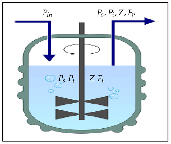
Figure 1. A bioreactor with a continuous stirring mechanism that continuously adds susceptible phytoplankton ($P_{in}$) and continuously removes the liquid culture ($P_s,P_i,Z,F_v$) at the same flow rate (D) [36,37,38,39].

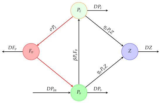
Figure 2. Schematic diagram of the desired system. $P_s$, $P_i$, Z, and $F_v$ describe the concentrations of susceptible and infected phytoplankton, zooplankton, and free viruses, respectively, in a chemostat.

Based on these ecological assumptions [35], we have the following system of nonlinear differential equations:

$$\begin{array}{c}\hfill \left\{\begin{array}{c}{\displaystyle {\dot{P}}_s=D{P}_{in}-\beta P_s{F}_v-{\displaystyle \frac{{\eta }_s}{Y}}{P}_{s}Z-D{P}_s,}\hfill \\ {\displaystyle {\dot{P}}_i=\beta P_s{F}_v-{\displaystyle \frac{{\eta }_i}{Y}}{P}_{i}Z-D{P}_i,}\hfill \\ {\displaystyle \dot{Z}=({\eta }_s{P}_s+{\eta }_i{P}_i)Z-DZ,}\hfill \\ {\displaystyle {\dot{F}}_v=\sigma P_i-D{F}_v.}\hfill \end{array}\right.\end{array}$$

(1)

with the positive initial condition $(P_s\left(0\right),P_i\left(0\right),Z\left(0\right),F_v\left(0\right))\in {\mathbb{R}}_{+}^4$.

$P_s\left(t\right)$ is the concentration of the susceptible phytoplankton in the chemostat at time t. $P_i\left(t\right)$ describes the concentration of the infected phytoplankton in the chemostat. $Z\left(t\right)$ reflects the concentration of zooplankton in the chemostat. $F_v\left(t\right)$ describes the concentration of free viruses in the chemostat. $P_{in}$ is the concentration of susceptible phytoplankton input into the chemostat. D is the dilution rate. ${\eta }_s$ and ${\eta }_i$ describe, respectively, the consumption rates of susceptible and infected phytoplankton by the zooplankton. $\beta$ is the saturated incidence rate. More details regarding the variables and parameters are given in Table 1. Note that the phytoplankton (either infected or not) are essential for the zooplankton’s growth and that the growth rate of zooplankton on susceptible phytoplankton increases with the susceptible phytoplankton concentration. Similarly, the growth rate of zooplankton on infected phytoplankton increases with the infected phytoplankton concentration. Furthermore, no infection can take place without the presence of free viruses in the chemostat. The growth rate of zooplankton on susceptible phytoplankton is more important than the one on the infected phytoplankton. The mortality rate of infected phytoplankton is greater than the mortality rate of susceptible phytoplankton.

Table 1. Description of the variables, functions, and parameters of system (1).

Variable	Description	Units
$P_s\left(t\right)$	Concentration of susceptible phytoplankton	g phytoplankton/L
$P_i\left(t\right)$	Concentration of infected phytoplankton	g phytoplankton/L
$Z\left(t\right)$	Concentration of zooplankton	g zooplankton/L
$F_v\left(t\right)$	Concentration of free viruses	g viruses/L
Parameter	Description	Units
D	Dilution rate	h−1
${\eta }_s$	Consumption rate of susceptible phytoplankton	h−1
${\eta }_i$	Consumption rate of infected phytoplankton	h−1
$P_{in}$	Susceptible phytoplankton input concentration	g phytoplankton/L
Y	Phytoplankton-to-zooplankton yield coefficient	g zooplankton/g phytoplankton
$\beta$	Saturated incidence rate	new infections/h
$\sigma$	Virus replication factor	g infected phytoplankton/g virus

We assume that

• A1 ${\eta }_i<{\eta }_s$.
• A2 $D<{\eta }_i{P}_{in}$.

Assumption A1 expresses that the growth rate of the zooplankton on the susceptible phytoplankton is more important than the one on the infected phytoplankton. Assumption A2 expresses that in the absence of the virus, the zooplankton can survive only on the susceptible phytoplankton.

3. Mathematical Results

In order to prove that the system (1) is well designed, it is necessary that the state variables $P_s\left(t\right)$, $P_i\left(t\right)$, $Z\left(t\right)$, and $F_v\left(t\right)$ remain nonnegative for all values of $t\ge 0$.

Proposition 1.

The compact set ${\displaystyle \Omega =\{(P_s,P_i,Z,F_v)\in {\mathbb{R}}_{+}^4/P_s+P_i+{\displaystyle \frac{Z}{Y}}=P_{in}, and F_v\le {\displaystyle \frac{\sigma }{D}}{P}_{in}\}}$ is positively invariant for system (1).

Proof. 

Since ${\dot{P}}_s=D{P}_{in}>0$ for $P_s=0$, ${\dot{P}}_i=\beta P_s{F}_v>0$ for $P_i=0$, $\dot{Z}=0$ for $Z=0$, and ${\dot{F}}_v=\sigma P_i>0$ for $F_v=0$, the solution of system (1) is nonnegative. By adding the first four equations of system (1), one obtains, for ${\displaystyle X=P_s+P_i+{\displaystyle \frac{Z}{Y}}-P_{in}}$, a single equation:

$$\begin{array}{ccccc}\hfill \begin{array}{ccc}{\displaystyle \dot{X}}\hfill & =\hfill & {\dot{P}}_s+{\dot{P}}_i+{\displaystyle \frac{\dot{Z}}{Y}}\hfill \end{array}& =& D\left(P_{in}-P_s-P_i-{\displaystyle \frac{Z}{Y}}\right)\hfill & =& -DX.\end{array}$$

Hence, $X\left(t\right)=X\left(0\right)e^{-Dt}$. Thus,

$$\begin{array}{c}\hfill \begin{array}{c}{\displaystyle P_s\left(t\right)+P_i\left(t\right)+{\displaystyle \frac{Z\left(t\right)}{Y}}-P_{in}=\left(P_s\left(0\right)+P_i\left(0\right)+{\displaystyle \frac{Z\left(0\right)}{Y}}-P_{in}\right)e^{-Dt}.}\hfill \end{array}\end{array}$$

(2)

Furthermore, we have ${\dot{F}}_v=\sigma P_i-D{F}_v\le \sigma P_{in}-D{F}_v\le D\left({\displaystyle \frac{\sigma }{D}}{P}_{in}-F_v\right)$. Hence,

$$\begin{array}{c}\hfill \begin{array}{c}{\displaystyle F_v\left(t\right)\le {\displaystyle \frac{\sigma }{D}}{P}_{in}+\left(F_v\left(0\right)-{\displaystyle \frac{\sigma }{D}}{P}_{in}\right)e^{-Dt}.}\hfill \end{array}\end{array}$$

(3)

Therefore, $\Omega$ is positively invariant for model (1) because all the variables are bounded since they are nonnegative.    □

3.1. The Ecosystem Without Free Viruses

In the absence of free viruses, we obtain the classical chemostat model that is well studied in [40] and is given hereafter.

$$\begin{array}{c}\hfill \left\{\begin{array}{c}{\displaystyle {\dot{P}}_s=D{P}_{in}-{\eta }_s{P}_s{\displaystyle \frac{Z}{Y}}-D{P}_s,}\hfill \\ {\displaystyle \dot{Z}={\eta }_s{P}_{s}Z-DZ.}\hfill \end{array}\right.\end{array}$$

(4)

This model is similar to the one studied in [41,42]. A modified Beddington type of interaction between phytoplankton and zooplankton is assumed in [41]. In [42], the impact of phytoplankton’s release of toxins on zooplankton and the fish predation of zooplankton are examined. By taking into account that environmental pollutants raise the mortality rate of both phytoplankton and zooplankton, Yu et al. [43] investigated a stochastic model.

The compact attractive set $\Omega$ of system (1) is reduced to ${\Omega }_0=\{(P_s,Z)\in {\mathbb{R}}_{+}^2/P_s+{\displaystyle \frac{Z}{Y}}=P_{in}\}$. System (4) admits a trivial steady state, ${\mathcal{E}}_0=\left(P_{in},0\right)$, and a nonnegative steady state, ${\mathcal{E}}^{*}=\left({\displaystyle \frac{D}{{\eta }_s}},Y\left(P_{in}-{\displaystyle \frac{D}{{\eta }_s}}\right)\right)$. Next, the local stability behaviors of the equilibrium points will be discussed.

Theorem 1.

1. 

There are no periodic orbits nor polycycles inside ${\Omega }_0$.

2. 

If $D<{\eta }_s{P}_{in}$ (Assumptions A1–A2), then the equilibrium point ${\mathcal{E}}^{*}$ exists and it is globally asymptotically stable, and ${\mathcal{E}}_0$ is a saddle point.

3. 

If ${\eta }_s{P}_{in}<D$, then the equilibrium point ${\mathcal{E}}_0$ is the unique equilibrium point of system (4), and it is globally asymptotically stable.

Proof. 

• Let $(P_s,Z)$ be a solution of (4) inside ${\Omega }_0$. By using the change in variables ${\xi }_1=P_s$ and ${\xi }_2=ln\left(Z\right)$, we obtain the following equations:

  $$\left\{\begin{array}{c}{\displaystyle {\dot{\xi }}_1=h_1({\xi }_1,{\xi }_2):=D{P}_{in}-D{\xi }_1-{\eta }_s{\xi }_1{\displaystyle \frac{e^{{\xi }_2}}{Y}},}\hfill \\ {\displaystyle {\dot{\xi }}_2=h_2({\xi }_1,{\xi }_2):={\eta }_s{\xi }_1-D.}\hfill \end{array}\right.$$

  (5)
  The divergence of system (4) is given by

  $${\displaystyle \frac{\partial h_1}{\partial {\xi }_1}+\frac{\partial h_2}{\partial {\xi }_2}=-D-{\eta }_s{\displaystyle \frac{e^{{\xi }_2}}{Y}}<0.}$$
  The Dulac criterion [40] states that there are no periodic solutions for (5), and so there are no periodic solutions for (4) inside ${\Omega }_0$.
• For $D<{\eta }_s{P}_{in}$ (Assumptions A1–A2), ${\mathcal{E}}^{*}$ exists and the Jacobian matrix at ${\mathcal{E}}^{*}$ is given by

  $$\begin{array}{c}\hfill {\mathcal{J}}^{*}=\left(\begin{array}{cc}-{\eta }_s{P}_{in}& -{\displaystyle \frac{D}{Y}}\\ Y({\eta }_s{P}_{in}-D)& 0\end{array}\right)\end{array}$$
  Since trace $\left({\mathcal{J}}^{*}\right)=-{\eta }_s{P}_{in}<0$ and det $\left({\mathcal{J}}^{*}\right)=D({\eta }_s{P}_{in}-D)>0$, both eigenvalues have a negative real part, and the equilibrium point ${\mathcal{E}}^{*}$ is therefore a locally asymptotically stable node. The Jacobian matrix evaluated at ${\mathcal{E}}_0$ is therefore given by

  $$\begin{array}{c}\hfill {\mathcal{J}}_0=\left(\begin{array}{cc}-D& -{\displaystyle \frac{{\eta }_s{P}_{in}}{Y}}\\ 0& {\eta }_s{P}_{in}-D\end{array}\right)\end{array}$$
  ${\mathcal{J}}_0$ admits two eigenvalues that are given by

  $${\lambda }_1=-D<0\mathrm{and}{\lambda }_2={\eta }_s{P}_{in}-D>0.$$
  Therefore, the equilibrium ${\mathcal{E}}_0$ is a saddle point with a stable manifold given by ${\Gamma }_0=]0,+\infty [\times \left\{0\right\}$. Let $P_s\left(0\right)\ge 0$ and $Z\left(0\right)>0$. By applying the Poincaré–Bendixon Theorem [40], the steady state ${\mathcal{E}}^{*}$ is found to be globally asymptotically stable.
• If ${\eta }_s{P}_{in}<D$, then ${\mathcal{E}}_0$ is the only steady state and is locally stable. Since any omega limit set is contained in the two-dimensional compact invariant set ${\Omega }_0$, and ${\mathcal{E}}_0$ lies on the boundary of ${\Omega }_0$, ${\mathcal{E}}_0$ is globally asymptotically stable according to the Poincaré-Bendixson Theorem.

   □

3.2. The Complete System

Let us return to the complete system (1). Let us calculate the steady states of system (1) satisfying

$$\begin{array}{c}\hfill \left\{\begin{array}{c}0=D{P}_{in}-\beta P_s{F}_v-{\eta }_s{P}_s{\displaystyle \frac{Z}{Y}}-D{P}_s,\hfill \\ 0=\beta P_s{F}_v-{\eta }_i{P}_i{\displaystyle \frac{Z}{Y}}-D{P}_i,\hfill \\ 0=({\eta }_s{P}_s+{\eta }_i{P}_i-D)Z,\hfill \\ 0=\sigma P_i-D{F}_v.\hfill \end{array}\right.\end{array}$$

(6)

• If $Z=0$, then we obtain a pure epidemic model with a steady state satisfying

  $$\begin{array}{c}\hfill \left\{\begin{array}{c}0=D{P}_{in}-\beta P_s{F}_v-D{P}_s,\hfill \\ 0=\beta P_s{F}_v-D{P}_i,\hfill \\ 0=\sigma P_i-D{F}_v.\hfill \end{array}\right.\end{array}$$

  (7)
  Then, $P_s=P_{in}-P_i$, and $F_v={\displaystyle \frac{\sigma }{D}}{P}_i$ with $\sigma \beta P_i(P_i-P_{in}+{\displaystyle \frac{D^2}{\sigma \beta }})=0$. Therefore, we obtain two equilibrium points, ${\mathcal{E}}_0=(P_{in},0,0,0)$ and ${\mathcal{E}}_1=\left({\displaystyle \frac{D^2}{\sigma \beta }},P_{in}-{\displaystyle \frac{D^2}{\sigma \beta }},0,{\displaystyle \frac{\sigma }{D}}{P}_{in}-{\displaystyle \frac{D}{\beta }}\right)$.
  The development of new infections and changes in the status of infected individuals are described by two equations in our example (Equations (2) and (4) in system (1)). We define the matrix F to represent the rate at which new infections develop in these two equations and V to represent the rate at which individuals are transferred into and out of these compartments by all other mechanisms in order to create the next generation matrix. Next, the non-singular matrix V and the nonnegative matrix F are provided by $F=\left[\begin{array}{cc}0& \beta P_{in}\\ \sigma & 0\end{array}\right]$ and $V=\left[\begin{array}{cc}D& 0\\ 0& D\end{array}\right]$. Therefore, $F{V}^{-1}=\left[\begin{array}{cc}0& {\displaystyle \frac{\beta P_{in}}{D}}\\ {\displaystyle \frac{\sigma }{D}}& 0\end{array}\right]$. The spectral radius of the next generation matrix FV⁻¹, which can be represented as follows, is the basic reproduction number of (1).

  $${\mathcal{R}}_0={\displaystyle \frac{\sqrt{\sigma \beta P_{in}}}{D}}.$$

  (8)
  Note that ${\mathcal{E}}_1=\left({\displaystyle \frac{D^2}{\sigma \beta }},{\displaystyle \frac{D^2}{\sigma \beta }}\left({\mathcal{R}}_0^2-1\right),0,{\displaystyle \frac{D}{\beta }}\left({\mathcal{R}}_0^2-1\right)\right)$. Therefore, ${\mathcal{E}}_1$ exists only if ${\mathcal{R}}_0>1$.
  The Jacobian matrix at ${\mathcal{E}}_0$ is given by

  $${\mathcal{J}}_0=\left(\begin{array}{cccc}-D& 0& -{\displaystyle \frac{{\eta }_s{P}_{in}}{Y}}& -\beta P_{in}\\ 0& -D& 0& \beta P_{in}\\ 0& 0& {\eta }_s{P}_{in}-D& 0\\ 0& \sigma & 0& -D\end{array}\right)$$

  where its characteristic polynomial is given by

  $$\begin{array}{c}\hfill \begin{array}{ccc}{P}_0\left(X\right)\hfill & =\hfill & -(X+D)\left({\eta }_s{P}_{in}-(X+D)\right)\times \left[{(X+D)}^2-\sigma \beta P_{in}\right].\hfill \end{array}\end{array}$$
  ${\mathcal{J}}_0$ admits $X_1=-D<0$, $X_2=-\sqrt{\sigma \beta P_{in}}-D<0$, $X_3={\eta }_s{P}_{in}-D>0$ according to Assumptions A1 and A2, and $X_4=\sqrt{\sigma \beta P_{in}}-D=D\left({\mathcal{R}}_0-1\right)$. Therefore, ${\mathcal{E}}_0$ is an unstable equilibrium point.
  The Jacobian matrix at ${\mathcal{E}}_1$ is given by

  $$\begin{array}{c}\hfill {\mathcal{J}}_1=\left(\begin{array}{cccc}-{\displaystyle \frac{\sigma \beta }{D}}{P}_{in}& 0& -{\displaystyle \frac{{\eta }_s{D}^2}{Y\sigma \beta }}& -{\displaystyle \frac{D^2}{\sigma }}\\ {\displaystyle \frac{\sigma \beta }{D}}{P}_{in}-D& -D& -{\displaystyle \frac{{\eta }_i{D}^2}{Y\sigma \beta }}\left({\mathcal{R}}_0^2-1\right)& {\displaystyle \frac{D^2}{\sigma }}\\ 0& 0& {\displaystyle \frac{{\eta }_s{D}^2}{\sigma \beta }}+{\displaystyle \frac{{\eta }_i{D}^2}{\sigma \beta }}\left({\mathcal{R}}_0^2-1\right)-D\hfill & 0\\ 0& \sigma & 0& -D\end{array}\right)\end{array}$$
  The characteristic polynomial is given by

  $$\begin{array}{c}\hfill \begin{array}{ccc}{P}_1\left(X\right)\hfill & =\hfill & -(X+D)\left({\displaystyle \frac{{\eta }_s{D}^2}{\sigma \beta }}+{\displaystyle \frac{{\eta }_i{D}^2}{\sigma \beta }}\left({\mathcal{R}}_0^2-1\right)-D-X)\right)\times \\ & & \left[X^2+\left(D+{\displaystyle \frac{\sigma \beta }{D}}{P}_{in}\right)X+D^2\left({\mathcal{R}}_0^2-1\right)\right].\end{array}\end{array}$$
  Note that

  $$\begin{array}{c}\hfill \begin{array}{ccc}{\displaystyle \frac{{\eta }_s{D}^2}{\sigma \beta }}+{\displaystyle \frac{{\eta }_i{D}^2}{\sigma \beta }}\left({\mathcal{R}}_0^2-1\right)-D\hfill & =\hfill & {\displaystyle \frac{P_{in}}{{\mathcal{R}}_0^2}}\left({\eta }_s+{\eta }_i\left({\mathcal{R}}_0^2-1\right)\right)-D\hfill \\ & >\hfill & {\displaystyle \frac{P_{in}}{{\mathcal{R}}_0^2}}\left({\eta }_i+{\eta }_i\left({\mathcal{R}}_0^2-1\right)\right)-D\hfill \\ & =\hfill & {\eta }_i{P}_{in}-D>0 \mathrm{according} \mathrm{to} \mathrm{Assumption} \mathbf{A}\mathbf{2}.\hfill \end{array}\end{array}$$
  Therefore, if ${\mathcal{R}}_0>1$, then ${\mathcal{E}}_1$ exists, and its Jacobian, ${\mathcal{J}}_1$, admits three negative eigenvalues and one positive eigenvalue, and thus ${\mathcal{E}}_1$ is an unstable equilibrium point.
• If $Z\ne 0$, then we have

  $$\begin{array}{c}\hfill \left\{\begin{array}{ccc}Z& =\hfill & {\displaystyle \frac{Y}{{\eta }_s}}\left({\eta }_s{P}_{in}-D+({\eta }_s-{\eta }_i)P_i\right)\hfill \\ F_v& =\hfill & {\displaystyle \frac{\sigma }{D}}{P}_i,\hfill \\ P_s& =\hfill & {\displaystyle \frac{D-{\eta }_i{P}_i}{{\eta }_s}}.\hfill \end{array}\right.\end{array}$$

  (9)

  with ${\displaystyle \frac{P_i}{D{\eta }_s}}\left((D({\eta }_s-{\eta }_i)-\sigma \beta ){\eta }_i{P}_i-D(D({\eta }_s-{\eta }_i)-\sigma \beta +{\eta }_s{\eta }_i{P}_{in})\right)=0$. We obtain two cases: The first case corresponds to the free viruses satisfying $P_i=0$, $F_v=0$, $P_s={\displaystyle \frac{D}{{\eta }_s}}$, and thus $Z={\displaystyle \frac{Y}{{\eta }_s}}\left({\eta }_s{P}_{in}-D\right)$. The disease-free equilibrium point is given by ${\mathcal{E}}_2=\left({\displaystyle \frac{D}{{\eta }_s}},0,{\displaystyle \frac{Y}{{\eta }_s}}\left({\eta }_s{P}_{in}-D\right),0\right)$. The second case satisfies $P_i^{*}={\displaystyle \frac{D(D({\eta }_s-{\eta }_i)-\sigma \beta +{\eta }_s{\eta }_i{P}_{in})}{{\eta }_i(D({\eta }_s-{\eta }_i)-\sigma \beta )}}$. Therefore, $Z^{*}={\displaystyle \frac{Y}{{\eta }_s}}\left({\eta }_s{P}_{in}-D+({\eta }_s-{\eta }_i)P_i^{*}\right)$, $F_v^{*}={\displaystyle \frac{\sigma (D({\eta }_s-{\eta }_i)-\sigma \beta +{\eta }_s{\eta }_i{P}_{in})}{{\eta }_i(D({\eta }_s-{\eta }_i)-\sigma \beta )}}$, and $P_s^{*}={\displaystyle \frac{D{\eta }_i{P}_{in}}{\sigma \beta -D({\eta }_s-{\eta }_i)}}$. We obtain the endemic equilibrium point that is given by ${\mathcal{E}}^{*}=\left(P_s^{*},P_i^{*},Z^{*},F_v^{*}\right)$. We aim to define the basic reproduction number again. Both the non-singular matrix V and the nonnegative matrix F are provided by $F=\left[\begin{array}{cc}0& {\displaystyle \frac{\beta D}{{\eta }_s}}\\ \sigma & 0\end{array}\right]$ and $V=\left[\begin{array}{cc}{\displaystyle \frac{{\eta }_i}{{\eta }_s}}\left({\eta }_s{P}_{in}-D\right)+D& 0\\ 0& D\end{array}\right]$. Therefore, $F{V}^{-1}=\left[\begin{array}{cc}0& {\displaystyle \frac{\beta }{{\eta }_s}}\\ {\displaystyle \frac{\sigma }{{\displaystyle \frac{{\eta }_i}{{\eta }_s}}\left({\eta }_s{P}_{in}-D\right)+D}}& 0\end{array}\right]$. The spectral radius of (1) is the spectral radius of the next generation matrix FV⁻¹, expressed as follows:

  $${\mathcal{R}}_1=\sqrt{{\displaystyle \frac{\beta \sigma }{{\eta }_i{\eta }_s{P}_{in}+D({\eta }_s-{\eta }_i)}}}.$$

  (10)
  Note that in a population where all phytoplankton are vulnerable to infection in the presence of zooplankton, the basic reproduction number, or ${\mathcal{R}}_1$, is the anticipated number of instances directly caused by one infected phytoplankton.
  Let ${\mathcal{J}}_2$ be the Jacobian matrix at ${\mathcal{E}}_2$.

  $$\begin{array}{c}\hfill {\mathcal{J}}_2=\left(\begin{array}{cccc}-{\eta }_s{P}_{in}& 0& -{\displaystyle \frac{D}{Y}}& -\beta {\displaystyle \frac{D}{{\eta }_s}}\\ 0& -{\displaystyle \frac{{\eta }_i}{{\eta }_s}}\left({\eta }_s{P}_{in}-D\right)-D& 0& \beta {\displaystyle \frac{D}{{\eta }_s}}\\ Y\left({\eta }_s{P}_{in}-D\right)& {\displaystyle \frac{{\eta }_{i}Y}{{\eta }_s}}\left({\eta }_s{P}_{in}-D\right)& 0& 0\\ 0& \sigma & 0& -D\end{array}\right)\end{array}$$
  The characteristic polynomial of ${\mathcal{J}}_2$ is given by

  $$\begin{array}{c}\hfill \begin{array}{ccc}{\mathcal{P}}_2\left(X\right)\hfill & =\hfill & \left|\begin{array}{cccc}-(X+{\eta }_s{P}_{in})& 0& -{\displaystyle \frac{D}{Y}}& -\beta {\displaystyle \frac{D}{{\eta }_s}}\\ 0& -{\displaystyle \frac{{\eta }_i}{{\eta }_s}}\left({\eta }_s{P}_{in}-D\right)-(X+D)& 0& \beta {\displaystyle \frac{D}{{\eta }_s}}\\ Y\left({\eta }_s{P}_{in}-D\right)& {\displaystyle \frac{{\eta }_{i}Y}{{\eta }_s}}\left({\eta }_s{P}_{in}-D\right)& -X& 0\\ 0& \sigma & 0& -(X+D)\end{array}\right|\hfill \\ & =\hfill & \left[X^2+\left(2D+{\displaystyle \frac{{\eta }_i}{{\eta }_s}}\left({\eta }_s{P}_{in}-D\right)\right)X+D\left(D+{\displaystyle \frac{{\eta }_i}{{\eta }_s}}\left({\eta }_s{P}_{in}-D\right)\right)-{\displaystyle \frac{D\sigma \beta }{{\eta }_s}}\right]\hfill \\ & & \left(X^2+{\eta }_s{P}_{in}X+D\left({\eta }_s{P}_{in}-D\right)\right)\hfill \end{array}\end{array}$$
  Note that $D\left(D+{\displaystyle \frac{{\eta }_i}{{\eta }_s}}\left({\eta }_s{P}_{in}-D\right)\right)-{\displaystyle \frac{D\sigma \beta }{{\eta }_s}}={\displaystyle \frac{D\sigma \beta }{{\eta }_s}}\left({\displaystyle \frac{D({\eta }_s-{\eta }_i)+{\eta }_i{\eta }_s{P}_{in}}{\sigma \beta }}-1\right)={\displaystyle \frac{D\sigma \beta }{{\eta }_s}}\left({\displaystyle \frac{1}{{\mathcal{R}}_1^2}}-1\right)$. Therefore, if ${\mathcal{R}}_1>1$, then ${\mathcal{E}}_2$ exists, and its Jacobian, ${\mathcal{J}}_2$, admits three negative eigenvalues (according to Assumptions A1–A2) and one positive eigenvalue, and thus ${\mathcal{E}}_2$ is an unstable equilibrium point. ${\mathcal{E}}_2$ is a stable equilibrium point only if ${\mathcal{R}}_1<1$.
  Let us discuss the existence and stability of the endemic equilibrium point ${\mathcal{E}}^{*}=(P_s^{*},P_i^{*},Z^{*},F_v^{*})$. Note that $P_s^{*}={\displaystyle \frac{D{\eta }_i{P}_{in}}{\sigma \beta -D({\eta }_s-{\eta }_i)}}>0$ means that $\sigma \beta >D({\eta }_s-{\eta }_i)$. Furthermore, we have $P_i^{*}={\displaystyle \frac{D\sigma \beta \left({\displaystyle \frac{1}{{\mathcal{R}}_1^2}}-1\right)}{{\eta }_i(D({\eta }_s-{\eta }_i)-\sigma \beta )}}$ and $F_v^{*}={\displaystyle \frac{{\sigma }^2\beta \left({\displaystyle \frac{1}{{\mathcal{R}}_1^2}}-1\right)}{{\eta }_i(D({\eta }_s-{\eta }_i)-\sigma \beta )}}$. Therefore, if ${\mathcal{R}}_1>1$, then $P_s^{*},P_i^{*},Z^{*},F_v^{*}>0$, and thus ${\mathcal{E}}^{*}=(P_s^{*},P_i^{*},Z^{*},F_v^{*})$ exists. Let ${\mathcal{J}}^{*}$ be the Jacobian matrix at ${\mathcal{E}}^{*}$, which is given by

  $$\begin{array}{c}\hfill {\mathcal{J}}^{*}=\left(\begin{array}{cccc}-\beta F_v^{*}-{\displaystyle \frac{{\eta }_s{Z}^{*}}{Y}}-D& 0& -{\displaystyle \frac{{\eta }_s{P}_s^{*}}{Y}}& -\beta P_s^{*}\\ \beta F_v^{*}& -{\displaystyle \frac{{\eta }_i{Z}^{*}}{Y}}-D& -{\displaystyle \frac{{\eta }_i{P}_i^{*}}{Y}}& \beta P_s^{*}\\ {\eta }_s{Z}^{*}& {\eta }_i{Z}^{*}& 0& 0\\ 0& \sigma & 0& -D\end{array}\right)\end{array}$$
  The characteristic polynomial of ${\mathcal{J}}^{*}$ is given by

  $$\begin{array}{c}\hfill \begin{array}{ccc}{\mathcal{P}}^{*}\left(X\right)\hfill & =\hfill & \left|\begin{array}{cccc}-\beta F_v^{*}-{\eta }_s{\displaystyle \frac{Z^{*}}{Y}}-D-X& 0& -{\displaystyle \frac{{\eta }_s{P}_s^{*}}{Y}}& -\beta P_s^{*}\\ \beta F_v^{*}& -{\eta }_i{\displaystyle \frac{Z^{*}}{Y}}-D-X& -{\displaystyle \frac{{\eta }_i{P}_i^{*}}{Y}}& \beta P_s^{*}\\ {\eta }_s{Z}^{*}& {\eta }_i{Z}^{*}& -X& 0\\ 0& \sigma & 0& -(X+D)\end{array}\right|\hfill \\ & =\hfill & {(X+D)}^2\left[X^2+\left({\eta }_i{\displaystyle \frac{Z^{*}}{Y}}+{\eta }_s{\displaystyle \frac{Z^{*}}{Y}}+D+\beta F_v^{*}\right)X+\left({\eta }_i^2{P}_i^{*}-{\eta }_i{\eta }_s{P}_i^{*}+{\eta }_i\beta F_v^{*}+{\eta }_s{\eta }_i{\displaystyle \frac{Z^{*}}{Y}}+{\eta }_{s}D\right){\displaystyle \frac{Z^{*}}{Y}}\right]\hfill \\ & & -{\displaystyle \frac{{\eta }_s\sigma \beta }{Y}}{P}_s^{*}{Z}^{*}X-{\displaystyle \frac{D{\eta }_s\sigma \beta }{Y}}{P}_s^{*}{Z}^{*}-\sigma \beta P_s^{*}{X}^2-D\sigma \beta P_s^{*}X\hfill \\ & =\hfill & X^4+a_3{X}^3+a_2{X}^2+a_{1}X+a_0,\hfill \end{array}\end{array}$$

  where $a_3=2D+({\eta }_s+{\eta }_i){\displaystyle \frac{Z^{*}}{Y}}+D+\beta F_v^{*}$,
  $a_2=2D\left(({\eta }_s+{\eta }_i){\displaystyle \frac{Z^{*}}{Y}}+\beta F_v^{*}\right)+3D^2+\left({\eta }_i^2{P}_i^{*}-{\eta }_i{\eta }_s{P}_i^{*}+{\eta }_i\beta F_v^{*}+{\eta }_s{\eta }_i{\displaystyle \frac{Z^{*}}{Y}}+{\eta }_{s}D\right){\displaystyle \frac{Z^{*}}{Y}}-\sigma \beta P_s^{*}$, $a_1=2D\left({\eta }_i^2{P}_i^{*}-{\eta }_i{\eta }_s{P}_i^{*}+{\eta }_i\beta F_v^{*}+{\eta }_s{\eta }_i{\displaystyle \frac{Z^{*}}{Y}}+{\eta }_{s}D\right){\displaystyle \frac{Z^{*}}{Y}}+D^2\left(({\eta }_s+{\eta }_i){\displaystyle \frac{Z^{*}}{Y}}+D+\beta F_v^{*}\right)-{\displaystyle \frac{{\eta }_s\sigma \beta }{Y}}{P}_s^{*}{Z}^{*}-D\sigma \beta P_s^{*}$, and $a_0=D^2\left[D({\eta }_s-{\eta }_i)+{\eta }_i{\eta }_s{P}_{in}+\sigma \beta \left(2{\displaystyle \frac{{\eta }_i{P}_i^{*}}{D}}-1\right)\right]{\displaystyle \frac{Z^{*}}{Y}}$. In order to use the Routh–Hurwitz criteria, one must see that $a_3>0$ and deduce that $a_0>0$ because $2{\displaystyle \frac{{\eta }_i{P}_i^{*}}{D}}=2{\displaystyle \frac{D({\eta }_s-{\eta }_i)-\sigma \beta +{\eta }_s{\eta }_i{P}_{in}}{D({\eta }_s-{\eta }_i)-\sigma \beta }}>1$. The calculation of the two other conditions was too large, so we used Maple 12 software to verify that $a_3{a}_2-a_1>0$ and $a_3(a_2{a}_1-a_3{a}_0)-a_1^2>0$, and thus we obtained the local stability of the equilibrium point ${\mathcal{E}}^{*}=(P_s^{*},P_i^{*},Z^{*},F_v^{*})$ once it exists (${\mathcal{R}}_1>1$).

For the following subsection, we aimed to study the global analysis for model (1), and we considered only the more important case where ${\eta }_i{\eta }_s{P}_{in}+({\eta }_s-{\eta }_i)D<\beta \sigma <{\displaystyle \frac{D^2}{P_{in}}}$, which leads to ${\mathcal{R}}_0<1<{\mathcal{R}}_1$. Therefore, all equilibrium points (${\mathcal{E}}_0$, ${\mathcal{E}}_1$, ${\mathcal{E}}_2$, and ${\mathcal{E}}^{*}$) exist such that ${\mathcal{E}}_0$, ${\mathcal{E}}_1$, and ${\mathcal{E}}_2$ are unstable equilibrium points; however, ${\mathcal{E}}^{*}$ is a stable equilibrium point.

3.3. Reduction to 3D

The 4D dynamics solutions (1) converged in the direction of $\Omega$. It was sufficient to limit the study of the dynamics (1) to the set $\Omega$ as our objective was to examine the asymptotic behavior of these solutions. This was because, according to Thieme’s findings [44], the trajectories’ asymptotic behavior would provide insight into the full dynamics (1). When restricted to $\Omega$, the system (1) becomes

$$\begin{array}{c}\hfill \left\{\begin{array}{c}{\displaystyle {\dot{P}}_i=\beta \left(P_{in}-P_i-{\displaystyle \frac{Z}{Y}}\right)F_v-{\displaystyle \frac{{\eta }_i}{Y}}{P}_{i}Z-D{P}_i,}\hfill \\ {\displaystyle \dot{Z}=\left[{\eta }_s\left(P_{in}-P_i-{\displaystyle \frac{Z}{Y}}\right)+{\eta }_i{P}_i-D\right]Z,}\hfill \\ {\displaystyle {\dot{F}}_v=\sigma P_i-D{F}_v.}\hfill \end{array}\right.\end{array}$$

(11)

where the solution $(P_i,Z,F_v)$ will be restricted by the subset of ${\mathbb{R}}_{+}^3$ given by

$$\Delta =\{(P_i,Z,F_v)\in {\mathbb{R}}_{+}^3/P_i+{\displaystyle \frac{Z}{Y}}\le P_{in}, \mathrm{and} F_v\le {\displaystyle \frac{\sigma }{D}}{P}_{in}\}.$$

Therefore, the reduced model (11) admits four equilibrium points in $\Delta$ that will be denoted as follows:

$$\begin{array}{c}\hfill \begin{array}{c}{\mathcal{Q}}_0=(0,0,0),{\mathcal{Q}}_1=\left(P_{in}-{\displaystyle \frac{D^2}{\sigma \beta }},0,{\displaystyle \frac{\sigma }{D}}{P}_{in}-{\displaystyle \frac{D}{\beta }}\right),{\mathcal{Q}}_2=\left(0,{\displaystyle \frac{Y}{{\eta }_s}}\left({\eta }_s{P}_{in}-D\right),0\right), \mathrm{and} {\mathcal{Q}}^{*}=\left(P_i^{*},Z^{*},F_v^{*}\right).\hfill \end{array}\end{array}$$

3.4. The Periodic Orbits on the Faces

Our goal in this section is to prove that there are no possible periodic orbits on the faces of the set $\Delta$, which will be useful later to prove that the solution will never converge to one of these faces [40,45].

• Let $(P_i,Z,F_v)$ be a solution of (11) on the face of $\Delta$ where $F_v=0$ that satisfies

  $$\begin{array}{c}\hfill \left\{\begin{array}{c}{\displaystyle {\dot{P}}_i=-{\displaystyle \frac{{\eta }_i}{Y}}{P}_{i}Z-D{P}_i,}\hfill \\ {\displaystyle \dot{Z}=\left[{\eta }_s\left(P_{in}-P_i-{\displaystyle \frac{Z}{Y}}\right)+{\eta }_i{P}_i-D\right]Z.}\hfill \end{array}\right.\end{array}$$

  (12)

  and belongs to ${\Delta }_{P_{i}Z}$, defined by

  $${\Delta }_{P_{i}Z}=\left\{(P_i,Z)\in {\mathbb{R}}_{+}^2:P_i+{\displaystyle \frac{Z}{Y}}\le P_{in}\right\}.$$
  It is easy to see that the axes $P_i=0$ and $Z=0$ are invariant. By applying the following change in the notations $y_1=P_i$ and $y_2=ln\left(Z\right)$ for $P_i,Z>0$, one obtains the following model:

  $$\left\{\begin{array}{cc}{\displaystyle {\dot{y}}_1=}\hfill & f_1(y_1,y_2):=-{\displaystyle \frac{{\eta }_i}{Y}}{y}_1{e}^{y_2}-D{y}_1,\hfill \\ {\displaystyle {\dot{y}}_2=}\hfill & f_2(y_1,y_2):={\eta }_s\left(P_{in}-y_1-{\displaystyle \frac{e^{y_2}}{Y}}\right)+{\eta }_i{y}_1-D.\hfill \end{array}\right.$$

  (13)
  Since ${\displaystyle \frac{\partial f_1}{\partial y_1}}+{\displaystyle \frac{\partial f_2}{\partial y_2}}=-D-({\eta }_s+{\eta }_i){\displaystyle \frac{e^{y_2}}{Y}}<0$, according to the Dulac criterion [40], there is not a periodic solution for system (13) or system (12). Consequently, there is no periodic solution for system (11) in the $P_{i}Z$ face ($F_v=0$).
• Let $(P_i,Z,F_v)$ to be a solution of (11) on the face of $\Delta$ where $P_i=0$ that satisfies

  $$\begin{array}{c}\hfill \left\{\begin{array}{c}{\displaystyle \dot{Z}=\left[{\eta }_s\left(P_{in}-{\displaystyle \frac{Z}{Y}}\right)-D\right]Z,}\hfill \\ {\displaystyle {\dot{F}}_v=-D{F}_v.}\hfill \end{array}\right.\end{array}$$

  (14)

  and belongs to ${\Delta }_{Z{F}_v}$, defined by

  $${\Delta }_{Z,F_v}=\left\{(Z,F_v)\in {\mathbb{R}}_{+}^2:{\displaystyle \frac{Z}{Y}}\le P_{in},F_v\le {\displaystyle \frac{\sigma }{D}}{P}_{in}\right\}.$$
  It is easy to see that the axes $Z=0$ and $F_v=0$ are invariant. By applying the following change in the notations $y_3=ln\left(Z\right)$ and $y_4=F_v$ for $P_s,F_v>0$, one obtains the following model:

  $$\left\{\begin{array}{cc}{\displaystyle {\dot{y}}_3=}\hfill & f_3(y_3,y_4):={\eta }_s\left(P_{in}-{\displaystyle \frac{e^{{\eta }_3}}{Y}}\right)-D,\hfill \\ {\displaystyle {\dot{y}}_4=}\hfill & f_4(y_3,y_4):=-D{y}_4.\hfill \end{array}\right.$$

  (15)
  Since ${\displaystyle \frac{\partial f_3}{\partial y_3}}+{\displaystyle \frac{\partial f_4}{\partial y_4}}=-{\eta }_s{\displaystyle \frac{e^{{\eta }_3}}{Y}}-D<0$, according to the Dulac criterion [40], there is not a periodic solution for system (15) or system (14). Consequently, there is no periodic solution for system (11) in the $Z{F}_v$ face ($P_i=0$).
• Let $(P_i,Z,F_v)$ be a solution of (11) on the face of $\Delta$ where $Z=0$ that satisfies

  $$\begin{array}{c}\hfill \left\{\begin{array}{cc}{\displaystyle {\dot{P}}_i=}\hfill & f_5(P_i,F_v):=\beta \left(P_{in}-P_i\right)F_v-D{P}_i,\hfill \\ {\displaystyle {\dot{F}}_v=}\hfill & f_6(P_i,F_v):=\sigma P_i-D{F}_v.\hfill \end{array}\right.\end{array}$$

  (16)

  and belongs to ${\Delta }_{P_i{F}_v}$, defined by

  $${\Delta }_{P_i{F}_v}=\left\{(P_i,F_v)\in {\mathbb{R}}_{+}^2:P_i\le P_{in},F_v\le {\displaystyle \frac{\sigma }{D}}{P}_{in}\right\}.$$
  It is easy to see that the axes $P_i=0$ and $F_v=0$ are invariant. Since ${\displaystyle \frac{\partial f_5}{\partial P_i}}+{\displaystyle \frac{\partial f_6}{\partial F_v}}=-\beta F_v-2D<0$, according to the Dulac criterion [40], there is not a periodic solution for system (16). Consequently, there is no periodic solution for system (11) in the $P_i{F}_v$ face ($Z=0$).

3.5. Persistence

The objective of this section is to demonstrate the persistence of the phytoplankton (either infected or not), the zooplankton, and the free viruses by proving the uniform persistence of system (11). We prove that each of the boundary steady states of system (11) are unstable. Therefore, by consistently applying the Butler–McGehee lemma [40], we employ the same proof as the one utilized in comparable circumstances in [45]. Next, we recall a definition pertaining to the Butler–McGehee lemma [40] and uniform persistence [45].

Definition 1

([45]). Consider the dynamics $\dot{q}=f\left(q\right)$ with the initial condition $q\left(0\right)=q_0\ge 0$ where $q\in {\mathbb{R}}^n$ and $f:{\mathbb{R}}^n\to {\mathbb{R}}^n$. The dynamics are said to be weakly persistent once ${\displaystyle \underset{t\to +\infty }{lim\; sup}q\left(t\right)>0}$. They are said to be persistent once ${\displaystyle \underset{t\to +\infty }{lim\; inf}q\left(t\right)>0}$. They are said to be uniformly persistent once $\exists \epsilon >0$, satisfying ${\displaystyle \underset{t\to +\infty }{lim\; inf}q\left(t\right)>\epsilon }$.

Lemma 1

(Butler–McGehee lemma [40]). Consider $f:{\mathbb{R}}^n\to {\mathbb{R}}^n$ to be a continuously differentiable function, $q^{*}$ to be a hyperbolic equilibrium point of the dynamics $\dot{q}=f\left(q\right)$ such that $q\left(0\right)=q_0\in {\mathbb{R}}^n$, ${\gamma }^{+}\left(q_0\right)$ to be the positive semi-orbit through $q_0$, and $\omega \left(q_0\right)$ to be the omega limit set of ${\gamma }^{+}\left(q_0\right)$. Assume that $q^{*}$ belongs to $\omega \left(q_0\right)$, such that it is not the entire omega limit set. Then, $\omega \left(q_0\right)$ should contain a non-trivial intersection of both the stable and unstable manifolds of $q^{*}$.

Theorem 2.

Model (11) is persistent.

Proof. 

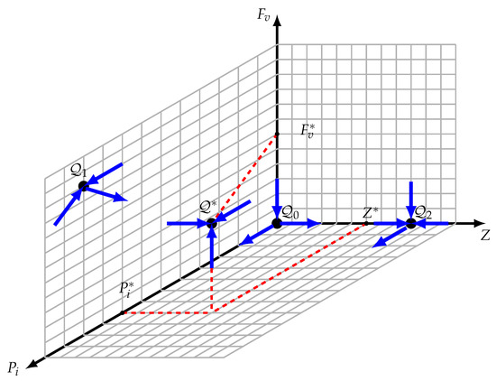
The stable and unstable manifolds of the border steady states are known and depicted in Figure 3 to clarify the argument since the three faces $P_{i}Z$, $Z{F}_v$, and $P_i{F}_v$ are invariant. Let $\overrightarrow{\mathbf{q}}=(P_i\left(t\right),Z\left(t\right),F_v\left(t\right))$ be a solution having the initial condition $\overrightarrow{\mathbf{q}}\left(0\right)=(P_i\left(0\right),Z\left(0\right),F_v\left(0\right))$ such that $P_i\left(0\right)$, $Z\left(0\right)$, and $F_v\left(0\right)>0$ are provided. We will demonstrate by contradiction that there is not a point with a zero coordinate in the omega limit set.

Figure 3. Equilibria configuration. ${\mathcal{Q}}_0$, ${\mathcal{Q}}_1$, and ${\mathcal{Q}}_2$ are unstable equilibrium points; however, $F^{*}$ is an asymptotically stable interior equilibrium.

• The omega limit set of ${\gamma }^{+}(\overrightarrow{\mathbf{q}}\left(0\right))$, represented as $\omega ({\gamma }^{+}(\overrightarrow{\mathbf{q}}\left(0\right))$, is assumed to include ${\mathcal{Q}}_0$. It should be noted that ${\mathcal{Q}}_0$ is a saddle point with a dimension of one stable manifold, $W^s\left({\mathcal{Q}}_0\right)$, that is limited to the $F_v$-axis. In this case, ${\mathcal{Q}}_0$ is not the whole omega limit set $\omega ({\gamma }^{+}(\overrightarrow{\mathbf{q}}\left(0\right))$. There is a point, $q^{*}\ne {\mathcal{Q}}_0$, in $\omega ({\gamma }^{+}(\overrightarrow{\mathbf{q}}\left(0\right)))\cap W^s\left({\mathcal{Q}}_0\right)$, according to the Butler–McGehee lemma [40]. Note that the $F_v$-axis is unbounded, but that $W^s\left({\mathcal{Q}}_0\right)$ is the $F_v$-axis. The omega limit set of any orbit of the system (11) should be bounded since all of its orbits are bounded (within the limited set $\Delta$). The existence of $q^{*}$ is contradicted by this. Consequently, ${\mathcal{Q}}_0\notin \omega ({\gamma }^{+}(\overrightarrow{\mathbf{q}}\left(0\right))$ should be confirmed.
• ${\mathcal{Q}}_1\in \omega ({\gamma }^{+}(\overrightarrow{\mathbf{q}}\left(0\right))$ is assumed. Likewise, $\left\{{\mathcal{Q}}_1\right\}$ should not be the complete omega limit set $\omega ({\gamma }^{+}(\overrightarrow{\mathbf{q}}\left(0\right)))$; hence, there is a point, $q^{*}\ne {\mathcal{Q}}_1$, inside $\omega ({\gamma }^{+}(\overrightarrow{\mathbf{q}}\left(0\right)))\cap W^s\left({\mathcal{Q}}_1\right)\setminus \left\{{\mathcal{Q}}_1\right\}$. Once $W^s\left({\mathcal{Q}}_1\right)$ is two-dimensional and completely contained in the $P_i{F}_v$ face, this point should be inside the $P_i{F}_v$ face. $\omega ({\gamma }^{+}(\overrightarrow{\mathbf{q}}\left(0\right))$ should contain the whole orbit via $q^{*}$, just like in the cases of ${\mathcal{Q}}_0$ and ${\mathcal{Q}}_2$. In Section 3.4, we demonstrated that there are no possible periodic orbits inside the $P_i{F}_v$ face. The orbit becomes unbounded once $\left\{{\mathcal{Q}}_1\right\}\notin \omega ({\gamma }^{+}(\overrightarrow{\mathbf{q}}\left(0\right)))$, which runs counter to the assertion that ${\mathcal{Q}}_1$ is inside $\omega ({\gamma }^{+}(\overrightarrow{\mathbf{q}}\left(0\right)))$.
• ${\mathcal{Q}}_2\in \omega ({\gamma }^{+}(\overrightarrow{\mathbf{q}}\left(0\right))$ is assumed. Given that ${\mathcal{Q}}_2$ is a saddle point, its stable manifold $W^s\left({\mathcal{Q}}_2\right)$ is limited to the $Z{F}_v$ plane and has two dimensions. Consequently, $\left\{{\mathcal{Q}}_2\right\}$ is not the whole omega limit set $\omega ({\gamma }^{+}(\overrightarrow{\mathbf{q}}\left(0\right))$. Accordingly, a point, $q^{*}\ne {\mathcal{Q}}_2$, exists inside $\omega ({\gamma }^{+}(\overrightarrow{\mathbf{q}}\left(0\right)))\cap W^s\left({\mathcal{Q}}_2\right)\setminus \left\{{\mathcal{Q}}_2\right\}$ according to the Butler–McGehee lemma [40]. Since $W^s\left({\mathcal{Q}}_2\right)$ lies entirely in the $Z{F}_v$ plane, and since the entire orbit through $q^{*}$ is in $\omega ({\gamma }^{+}(\overrightarrow{\mathbf{q}}\left(0\right)))$, this orbit is thus unbounded, which contradicts the fact that ${\mathcal{Q}}_2$ is inside $\omega ({\gamma }^{+}(\overrightarrow{\mathbf{q}}\left(0\right)))$.

Assume that $\widehat{\mathbf{q}}\in \omega ({\gamma }^{+}(\overrightarrow{\mathbf{q}}\left(0\right)))$, and let $\widehat{\mathbf{q}}=({\widehat{P}}_i\left(t\right),\widehat{Z}\left(t\right),{\widehat{F}}_v\left(t\right))$, with at least one of the components ${\widehat{P}}_i\left(t\right)$, $\widehat{Z}\left(t\right)$, and ${\widehat{F}}_v\left(t\right)$ being zero. Therefore, $\omega ({\gamma }^{+}(\overrightarrow{\mathbf{q}}\left(0\right))$ should contain the full orbit that passes over $\widehat{\mathbf{q}}$. Nevertheless, since there is no potential periodic orbit, the orbit should converge to one of the boundary equilibrium points since it should lie completely inside the $P_{i}Z$, $Z{F}_v$, or $P_i{F}_v$ faces. The idea that all boundary equilibrium points are unstable is thus contradicted by the fact that this boundary equilibrium point is inside $\omega ({\gamma }^{+}(\overrightarrow{\mathbf{q}}\left(0\right))$. Consequently, we have demonstrated that every component of the trajectory is bigger than zero.

$$\underset{t\to \infty }{lim\; inf}{P}_i\left(t\right)>0,\underset{t\to \infty }{lim\; inf}Z\left(t\right)>0\mathrm{and}\underset{t\to \infty }{lim\; inf}{F}_v\left(t\right)>0,$$

and so system (11) is persistent (see [45] (Section 4.3) for another application).    □

3.6. Uniform Persistence of System (7)

Keep in mind that persistence is the same as uniform persistence in a number of biological model scenarios [46]. Remember the theory in [46] regarding a dynamical system, $\mathcal{D}$, for which ${\mathbb{R}}_{+}^3$ and $\partial {\mathbb{R}}_{+}^3$ are both invariant. This is relevant to our situation. Thus, under the following criteria, $\mathcal{D}$ is uniformly persistent:

• The dynamics $\mathcal{D}$ are weakly persistent;
• The dynamics $\mathcal{D}$ are dissipative;
• The restriction of $\mathcal{D}$ to $\partial {\mathbb{R}}_{+}^3$ is isolated;
• The restriction of $\mathcal{D}$ to $\partial {\mathbb{R}}_{+}^3$ is acyclic.

Assume that the dynamics on $\Omega$ defined in Proposition 1 are denoted by $\mathcal{D}$. $\partial \Omega$ is not invariant; however, when $\partial \Omega ={\Omega }_1\cup {\Omega }_2$ and $\mathcal{D}$ is invariant on ${\Omega }_1$ but repellent in the interior of $\Omega$ on ${\Omega }_2$, the theorem in [46], as applied in [45,47], should be applied in our case, provided that both conditions 3 and 4 are met when restricting $\mathcal{D}$ to ${\Omega }_1$. The invariant set $\Omega$ is bounded for our system. Consequently, condition 1 is met. According to Theorem 2, condition 2 is true since the persistence implies weak persistence.

The union of the equilibrium points also covers the omega limit sets of ${\Omega }_1$, and as all border equilibrium points are hyperbolic, each one is the largest invariant set in its neighborhood, verifying that condition 3 is met. Since there is no cyclical link between the boundary equilibrium points, condition 4 is likewise met. As stated in the subsequent theorem, we consequently infer the uniform persistence of model (11).

Theorem 3.

Model (11) is uniformly persistent, i.e., $\exists \zeta >0$, satisfying

$$\underset{s\to \infty }{lim\; inf}{P}_i\left(s\right)>\zeta ,\underset{s\to \infty }{lim\; inf}Z\left(s\right)>\zeta ,\underset{s\to \infty }{lim\; inf}{F}_v\left(s\right)>\zeta .$$

3.7. Uniform Persistence of System (1)

To demonstrate that model (1) is also uniformly persistent, let us extend the persistence findings. If ${\overrightarrow{\mathbf{q}}}_0=(P_s\left(0\right),P_i\left(0\right),Z\left(0\right),F_v\left(0\right))$ with the provided data $P_s\left(0\right)\ge 0,P_i\left(0\right)\ge 0,Z\left(0\right)\ge 0$, and $F_v\left(0\right)\ge 0$, we obtain $\omega ({\overrightarrow{\mathbf{q}}}_0)\in \Omega$. Nevertheless, there is a time sequence ($s_n$) converging to ∞, where the corresponding solution is converging to $\overrightarrow{\mathbf{p}}$, and $\overrightarrow{\mathbf{p}}\in {\mathbb{R}}_{+}^4\setminus \Omega$. This suggests that $\Omega$ is not globally attractive, which runs counter to the results given in Proposition 1. Additionally, suppose that $\omega ({\overrightarrow{\mathbf{q}}}_0)$ contains a point on a boundary face where one of the variables $P_i,Z$, or $F_v$ is zero; hence, the complete orbit that passes through this point should be inside $\omega ({\overrightarrow{\mathbf{q}}}_0)$. Consequently, $\Omega$ contains the full omega limit set $\omega ({\overrightarrow{\mathbf{q}}}_0)$.

Thus, the following theorem is the main finding that we can deduce.

Theorem 4.

Model (1) is uniformly persistent.

In the next section, the sensitivity analysis of the basic reproduction number will be discussed.

4. Sensitivity Analysis

Finding and measuring the input parameters’ contribution to the model’s outcomes is the goal of sensitivity analysis [48]. A sensitivity index is typically used to quantify the sensitivity of a variable to the parameters. This enables us to ascertain the relative change in a variable after the value of a parameter is altered. Specifically, we are able to identify the parameters that most affect the fundamental reproduction number ${\mathcal{R}}_1$. Partial derivatives were used to determine the sensitivity indices since ${\mathcal{R}}_1$ is a differentiable function to certain parameters [48]. We aimed to perform a sensitivity analysis for the basic reproduction number ${\mathcal{R}}_1$ by identifying its contribution to determining the stability of the persistence equilibrium ${\mathcal{E}}^{*}$. The sensitivity indices of ${\mathcal{R}}_1$ with respect to a parameter, p, are given by [48]

$$I_p={\displaystyle \frac{\partial {\mathcal{R}}_1}{\partial p}}\times {\displaystyle \frac{p}{{\mathcal{R}}_1}}.$$

The explicit expression of ${\mathcal{R}}_1$ is given by ${\mathcal{R}}_1=\sqrt{{\displaystyle \frac{\beta \sigma }{{\eta }_i{\eta }_s{P}_{in}+{\eta }_{s}D-{\eta }_{i}D}}}$.

By considering the model’s parameters, given in Table 2, we found the sensitivity indices of ${\mathcal{R}}_1$ with respect to the model’s parameters, which are given hereafter in Table 3.

Table 2. The parameter values used in all numerical simulations were selected arbitrarily. There is no biological meaning to these values.

Parameter	Y	${\mathit{\eta }}_{\mathit{s}}$	${\mathit{\eta }}_{\mathit{i}}$	${\mathit{P}}_{\mathbf{in}}$	D	$\mathit{\beta }$	$\mathit{\sigma }$
Value	$0.5$	$0.6$	$0.5$	8	$2.5$	$0.6$	$4.7$

Table 3. Sensitivity of ${\mathcal{R}}_1$ to the model’s parameters.

Parameter, p	Sensitivity Index, ${\mathit{I}}_{\mathit{p}}$	Value
$\sigma$	${\displaystyle \frac{1}{2}}$	0.5
$\beta$	${\displaystyle \frac{1}{2}}$	0.5
D	${\displaystyle \frac{-D({\eta }_s-{\eta }_i)}{2{\eta }_i{\eta }_s{P}_{in}+2D({\eta }_s-{\eta }_i)}}$	−0.0472
${\eta }_i$	${\displaystyle \frac{-{\eta }_i{\eta }_s{P}_{in}+D{\eta }_i}{2{\eta }_i{\eta }_s{P}_{in}+2D({\eta }_s-{\eta }_i)}}$	−0.217
$P_{in}$	${\displaystyle \frac{-{\eta }_i{\eta }_s{P}_{in}}{2{\eta }_i{\eta }_s{P}_{in}+2D({\eta }_s-{\eta }_i)}}$	−0.4528
${\eta }_s$	${\displaystyle \frac{-{\eta }_i{\eta }_s{P}_{in}-D{\eta }_s}{2{\eta }_i{\eta }_s{P}_{in}+2D({\eta }_s-{\eta }_i)}}$	−0.6712

In relation to $\sigma$ and $\beta$, the sensitivity indices of ${\mathcal{R}}_1$ are positive; however, the sensitivity indices of ${\mathcal{R}}_1$ with respect to D, ${\eta }_i$, $P_{in}$, and ${\eta }_s$ are negative in Figure 4. Therefore, an increase in the values of parameters $\sigma$ or $\beta$ leads to an increase in the value of ${\mathcal{R}}_1$; however, an increase in the values of parameters D, ${\eta }_i$, $P_{in}$, and ${\eta }_s$ leads to a decrease in the value of ${\mathcal{R}}_1$. According to the values in Table 3, increasing (or decreasing) $\sigma$ and $\beta$ by $100\%$ will increase (or decrease) the ${\mathcal{R}}_1$ value by $50\%$. However, increasing (or decreasing) D by $100\%$ will decrease (or increase) the ${\mathcal{R}}_1$ value by $4.72\%$. Similarly, increasing (or decreasing) ${\eta }_i$ by $100\%$ will decrease (or increase) the ${\mathcal{R}}_1$ value by $21.7\%$. Similarly, increasing (or decreasing) $P_{in}$ by $100\%$ will decrease (or increase) the ${\mathcal{R}}_1$ value by $45.28\%$. Finally, increasing (or decreasing) ${\eta }_s$ by $100\%$ will decrease (or increase) the ${\mathcal{R}}_1$ value by $67.12\%$. Note that ${\mathcal{R}}_1$ is not sensitive to the other parameters of system (1).

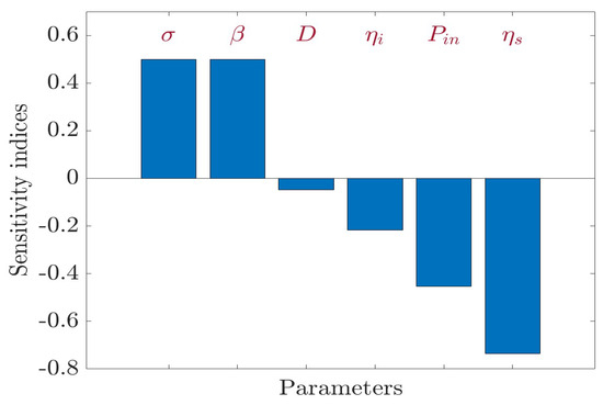
Figure 4. Sensitivity analysis for ${\mathcal{R}}_1$.

In the next section, the optimal control problem will be discussed.

5. Optimal Control Strategy

This section’s objective is to suggest an optimal strategy to adjust the concentration of the zooplankton, $Z\left(t\right)$, to the desired value, $Z_d$, and minimize the virus concentration inside the reactor while maintaining an optimal dilution rate, $D\left(t\right)$, throughout the process. Several strategies have been applied in some mathematical studies on the anaerobic digestion process with and without the influence of leachate recirculation [49,50]. We will take into account an objective functional that reflects the adjustment of the concentration of the zooplankton, $Z\left(t\right)$, to the desired value, $Z_d$, maintaining the validity of the biological process. Let $D\left(t\right)$ be the control function representing the dilution rate (cost). The set of permissible controls is provided by

$${\mathbf{P}}_{\mathbf{ad}}=\{D\left(t\right):0<D^{min}\le D\left(t\right)\le D^{max},0\le t\le T,D\left(t\right)\mathrm{is}\mathrm{Lebesgue}\mathrm{measurable}\},$$

minimizing the objective function considered hereafter:

$$J\left(D\right)={\displaystyle \frac{{\alpha }_1}{2}}{\int }_0^T{(Z-Z_d)}^2\left(t\right)dt+{\displaystyle \frac{{\alpha }_2}{2}}{\int }_0^T{F}_v^2\left(t\right)dt+{\displaystyle \frac{{\alpha }_3}{2}}{\int }_0^T{D}^2\left(t\right)dt.$$

By selecting suitable positive balancing constants, ${\alpha }_1$, ${\alpha }_2$, and ${\alpha }_3$, the goal is to attain the desired value of the concentration of the zooplankton, $Z\left(t\right)$, minimize the virus concentration inside the reactor, and also minimize the cost of the dilution rate, $D\left(t\right)$.

We demonstrate the existence of both the optimal control and the corresponding states using classic results [51]. For $\varpi ={\left(P_s,P_i,Z,F_v\right)}^t$, system (1) can be transformed as the following:

$$\begin{array}{c}\hfill \begin{array}{c}{\displaystyle \dot{\varpi }=\varrho \left(\varpi \right)-\alpha \left(\varpi \right)=\upsilon \left(\varpi \right)}\hfill \end{array}\end{array}$$

(17)

with $\alpha \left(\varpi \right)=D\varpi$ and $\varrho \left(\varpi \right)=\left(\begin{array}{c}D{P}_{in}-\beta P_s{F}_v-{\eta }_s{P}_s{\displaystyle \frac{Z}{Y}}\\ \beta P_s{F}_v-{\eta }_i{P}_i{\displaystyle \frac{Z}{Y}}\\ ({\eta }_s{P}_s+{\eta }_i{P}_i)Z\\ \sigma P_i\end{array}\right)$.

Note that $\varrho$ satisfies

$$\begin{array}{c}\hfill \begin{array}{ccc}\hfill \parallel \varrho \left({\varpi }^{\prime }\right)-\varrho \left(\varpi \right){\parallel }_1& =\hfill & |\beta P_s^{\prime }{F}_v^{\prime }-\beta P_s{F}_v+{\eta }_s{P}_s^{\prime }{\displaystyle \frac{Z^{\prime }}{Y}}-{\eta }_s{P}_s{\displaystyle \frac{Z}{Y}}|\hfill \\ & & +|\beta P_s{F}_v-\beta P_s^{\prime }{F}_v^{\prime }+{\eta }_i{P}_i^{\prime }{\displaystyle \frac{Z^{\prime }}{Y}}-{\eta }_i{P}_i{\displaystyle \frac{Z}{Y}}|\hfill \\ & & +|{\eta }_s{P}_{s}Z-{\eta }_s{P}_s^{\prime }{Z}^{\prime }+{\eta }_i{P}_{i}Z-{\eta }_i{P}_i^{\prime }{Z}^{\prime }|+\left|\sigma (P_i-P_i^{\prime })\right|\hfill \\ & \le & 2\beta P_{in}|F_v^{\prime }-F_v|+(\frac{{\eta }_s}{Y}+\frac{{\eta }_i}{Y}+{\eta }_s+{\eta }_i)P_{in}|Z^{\prime }-Z|\hfill \\ & & +(2\frac{\beta \sigma P_{in}}{D}+{\eta }_{i}Y{P}_{in}+{\eta }_i{P}_{in}+\sigma )|P_i-P_i^{\prime }|\hfill \\ & & +({\eta }_{s}Y+{\eta }_s)P_{in}|P_s-P_s^{\prime }|\hfill \\ & \le & M\parallel {\varpi }_1-{\varpi }_2{\parallel }_1\hfill \end{array}\end{array}$$

where

$$M=max\left(2\beta P_{in},({\displaystyle \frac{{\eta }_s}{Y}}+{\displaystyle \frac{{\eta }_i}{Y}}+{\eta }_s+{\eta }_i)P_{in},\left(2{\displaystyle \frac{\beta \sigma P_{in}}{D}}+{\eta }_{i}Y{P}_{in}+{\eta }_i{P}_{in}+\sigma \right),\left({\eta }_{s}Y+{\eta }_s\right)P_{in}\right).$$

Since ${\parallel \alpha \left({\varpi }^{\prime }\right)-\alpha \left(\varpi \right){\parallel }_1=D\parallel {\varpi }^{\prime }-\varpi \parallel }_1$, ${\displaystyle \parallel \upsilon \left({\varpi }^{\prime }\right)-\upsilon \left(\varpi \right){\parallel }_1\le K\parallel {\varpi }^{\prime }-\varpi {\parallel }_1}$ with $K=max(M,D)$, and therefore $\upsilon$ is a uniformly Lipschitz continuous function.

Consequently, a unique solution is admitted by system (17). It is possible to construct the optimal control problem for dynamics (17) subject to the minimization of the objective functional J in terms of the Hamiltonian function by using Pontryagin’s maximum principle [51,52,53].

$$\begin{array}{c}\hfill \begin{array}{ccc}H\hfill & =\hfill & {\displaystyle \frac{{\alpha }_1}{2}}{(Z-Z_d)}^2+{\displaystyle \frac{{\alpha }_3}{2}}{D}^2+{\displaystyle \frac{{\alpha }_2}{2}}{F}_v^2+{\lambda }_1{\dot{P}}_s+{\lambda }_2{\dot{P}}_i+{\lambda }_3\dot{Z}+{\lambda }_4{\dot{F}}_v\hfill \\ & =\hfill & {\displaystyle \frac{{\alpha }_1}{2}}{(Z-Z_d)}^2+{\displaystyle \frac{{\alpha }_2}{2}}{F}_v^2+{\displaystyle \frac{{\alpha }_3}{2}}{D}^2+{\lambda }_1\left(D{P}_{in}-\beta P_s{F}_v-{\eta }_s{P}_s{\displaystyle \frac{Z}{Y}}-D{P}_s\right)\hfill \\ & & +{\lambda }_2\left(\beta P_s{F}_v-{\eta }_i{P}_i{\displaystyle \frac{Z}{Y}}-D{P}_i\right)+{\lambda }_3\left({\eta }_s{P}_s+{\eta }_i{P}_i-D\right)Z+{\lambda }_4\left(\sigma P_i-D{F}_v\right).\hfill \end{array}\end{array}$$

(18)

The adjoint system provided below considers the adjoint variables ${\lambda }_1,{\lambda }_2,{\lambda }_3$, and ${\lambda }_4$, which correspond to the states $P_s,P_i,Z$, and $F_v$ with a given optimum control, D.

$$\left\{\begin{array}{ccc}{\dot{\lambda }}_1\hfill & =\hfill & -{\displaystyle \frac{\partial H}{\partial P_s}}={\lambda }_1\left(\beta F_v+{\eta }_s{\displaystyle \frac{Z}{Y}}+D\right)-{\lambda }_2\beta F_v-{\lambda }_3{\eta }_{s}Z,\hfill \\ {\dot{\lambda }}_2\hfill & =\hfill & -{\displaystyle \frac{\partial H}{\partial P_i}}={\lambda }_2\left({\eta }_i{\displaystyle \frac{Z}{Y}}+D\right)-{\lambda }_3{\eta }_{i}Z-{\lambda }_4\sigma ,\hfill \\ {\dot{\lambda }}_3\hfill & =\hfill & -{\displaystyle \frac{\partial H}{\partial Z}}=-{\alpha }_1(Z-Z_d)+{\lambda }_1{\displaystyle \frac{{\eta }_s{P}_s}{Y}}+{\lambda }_2{\displaystyle \frac{{\eta }_i{P}_i}{Y}}-{\lambda }_3\left({\eta }_s{P}_s+{\eta }_i{P}_i-D\right),\hfill \\ {\dot{\lambda }}_4\hfill & =\hfill & -{\displaystyle \frac{\partial H}{\partial F_v}}=-{\alpha }_2{F}_v+{\lambda }_1\beta P_s-{\lambda }_2\beta P_s+D{\lambda }_4.\hfill \end{array}\right.$$

with ${\lambda }_1\left(T\right)=0$, ${\lambda }_2\left(T\right)=0$, ${\lambda }_3\left(T\right)=0$, and ${\lambda }_4\left(T\right)=0$.

At D, the Hamiltonian is reduced in relation to the control variable. The Hamiltonian’s derivative is provided by

$${\displaystyle \frac{\partial H}{\partial D}}={\alpha }_{3}D+{\lambda }_1\left(P_{in}-P_s\right)-{\lambda }_2{P}_i-{\lambda }_{3}Z-{\lambda }_4{F}_v.$$

Therefore, ${\displaystyle \frac{\partial H}{\partial D}}=0$ admits the solution

$$D^{*}\left(t\right)={\displaystyle \frac{{\lambda }_1(P_s-P_{in})+{\lambda }_2{P}_i+{\lambda }_{3}Z+{\lambda }_4{F}_v}{{\alpha }_3}}$$

provided that ${\alpha }_3\ne 0$ and

$$D^{min}\le {\displaystyle \frac{{\lambda }_1(P_s-P_{in})+{\lambda }_2{P}_i+{\lambda }_{3}Z+{\lambda }_4{F}_v}{{\alpha }_3}}\le D^{max}.$$

In summary, the characterization of the control is

$$\begin{array}{c}\hfill \left\{\begin{array}{c}\mathrm{if} {\displaystyle \frac{\partial H}{\partial D}}<0 \mathrm{at} t, \mathrm{then} D\left(t\right)=D^{max},\hfill \\ \mathrm{if} {\displaystyle \frac{\partial H}{\partial D}}>0 \mathrm{at} t, \mathrm{then} D\left(t\right)=D^{min},\hfill \\ \mathrm{if} {\displaystyle \frac{\partial H}{\partial D}}=0 \mathrm{at} t, \mathrm{then} D\left(t\right)=D^{*}\left(t\right)={\displaystyle \frac{{\lambda }_1(P_s-P_{in})+{\lambda }_2{P}_i+{\lambda }_{3}Z+{\lambda }_4{F}_v}{{\alpha }_3}}.\hfill \end{array}\right.\end{array}$$

In the next section, several numerical examples will be given confirming the theoretical findings.

6. Numerical Investigations

We provide several numerical examples to support the results achieved. Using MATLAB R2024a software, the Runge–Kutta–Fehlberg method was the numerical approach used to solve the model (ode45). The parameter values used in all numerical simulations were selected arbitrarily for each case.

6.1. Direct Problem

A number of numerical examples for system (1) are presented for a fixed dilution rate. In Figure 5 and Figure 6, all components persist and then the positive steady state ${\mathcal{E}}^{*}$ is stable. In Figure 7 and Figure 8, the zooplankton go extinct and the other variables persist. In Figure 9 and Figure 10, the system becomes disease-free and the phytoplankton and zooplankton persist. In Figure 11 and Figure 12, both the infectious virus and the zooplankton go extinct, and the susceptible phytoplankton persists.

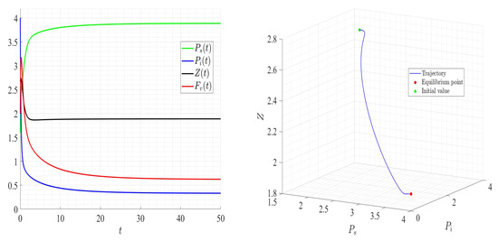
Figure 5. Dynamics of model (1); the components’ behavior (left) and the $P_s-P_i-Z$ comportment (right) for ${\eta }_s=0.6$, ${\eta }_i=0.5$, $Y=0.5$, $P_{in}=8$, $D=2.5$, $\beta =0.6$, and $\sigma =4.7$, with ${\mathcal{R}}_1=1.13>1$. The green dot (right) is the initial condition, and the red dot (right) is the equilibrium point in the space $(P_s,P_i,Z)$.

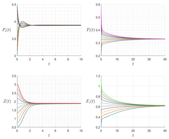
Figure 6. The dynamics of the variables for a range of initial values for ${\eta }_s=0.6$, ${\eta }_i=0.5$, $Y=0.5$, $P_{in}=8$, $D=2.5$, $\beta =0.6$, and $\sigma =4.7$, with ${\mathcal{R}}_1=1.13>1$. The various initial conditions are shown by the various colors.

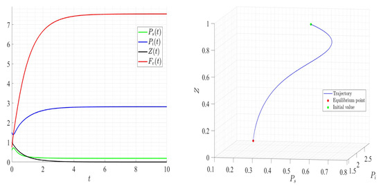
Figure 7. Dynamics of model (1); the components’ behavior (left) and the $P_s-P_i-Z$ comportment (right) for ${\eta }_s=0.6$, ${\eta }_i=0.5$, $Y=0.5$, $P_{in}=3$, $D=2.5$, $\beta =5$, and $\sigma =6.7$, with ${\mathcal{R}}_0=4.01>1$. The green dot (right) is the initial condition, and the red dot (right) is the equilibrium point in the space $(P_s,P_i,Z)$.

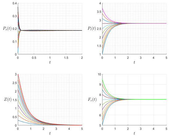
Figure 8. The dynamics of the variables for a range of initial values for ${\eta }_s=0.6$, ${\eta }_i=0.5$, $Y=0.5$, $P_{in}=3$, $D=2.5$, $\beta =5$, and $\sigma =6.7$, with ${\mathcal{R}}_0=4.01>1$. The various initial conditions are shown by the various colors.

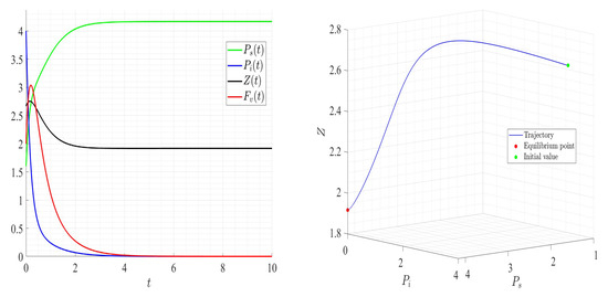
Figure 9. Dynamics of model (1); the components’ behavior (left) and the $P_s-P_i-Z$ comportment (right) for ${\eta }_s=0.6$, ${\eta }_i=0.5$, $Y=0.5$, $P_{in}=8$, $D=2.5$, $\beta =0.2$, and $\sigma =4.7$, with ${\mathcal{R}}_1=0.66<1$. The green dot (right) is the initial condition, and the red dot (right) is the equilibrium point in the space $(P_s,P_i,Z)$.

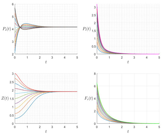
Figure 10. The dynamics ofthe variables for a range of initial values for ${\eta }_s=0.6$, ${\eta }_i=0.5$, $Y=0.5$, $P_{in}=8$, $D=2.5$, $\beta =0.2$, and $\sigma =4.7$, with ${\mathcal{R}}_1=0.66<1$. The various initial conditions are shown by the various colors.

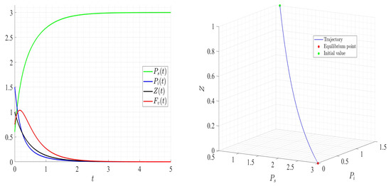
Figure 11. Dynamics of model (1); the components’ behavior (left) and the $P_s-P_i-Z$ comportment (right) for ${\eta }_s=0.6$, ${\eta }_i=0.5$, $Y=0.5$, $P_{in}=3$, $D=3.5$, $\beta =0.2$, and $\sigma =4.7$, with ${\mathcal{R}}_0=0.48<1$. The green dot (right) is the initial condition, and the red dot (right) is the steady state in the space $(P_s,P_i,Z)$.

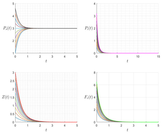
Figure 12. The dynamics of the variables for a range of initial values for ${\eta }_s=0.6$, ${\eta }_i=0.5$, $Y=0.5$, $P_{in}=3$, $D=3.5$, $\beta =0.2$, and $\sigma =4.7$, with ${\mathcal{R}}_0=0.48<1$. The various initial conditions are shown by the various colors.

6.2. Optimal Control Problem

The dilution rate, D, is assumed to be a time-varying function, $D\left(t\right)$, in the following examples. Its initial value is $D\left(0\right)=2.75$, and its bounds are $D^{min}=0.5$ and $D^{max}=5$. The initial state value $x_0=(1.6,4,2.6667,2)$ is taken into consideration. Appendix A provides the numerical scheme utilized for the control problem. Figure 13, Figure 14 and Figure 15 demonstrate how smooth the ideal solution is. If we increase the ${\alpha }_1$ values, the control values decrease; if we increase the ${\alpha }_3$ and ${\alpha }_1$ values, the control values increase. Keep in mind that altering the values of ${\alpha }_1$ and ${\alpha }_3$ does not affect the final zooplankton concentration value. The best approach involves lowering the virus content within the chemostat for ideal dilution rate values (costs) and adjusting the zooplankton concentration to an ideal value.

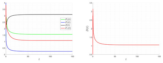
Figure 13. Impact of the optimal dilution rate on the system for ${\alpha }_1=1$, ${\alpha }_2=1$, and ${\alpha }_3=1$.

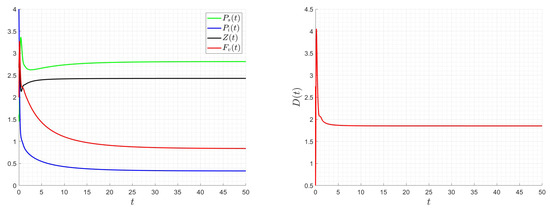
Figure 14. Impact of the optimal dilution rate on the system for ${\alpha }_1=10$, ${\alpha }_2=1$, and ${\alpha }_3=1$.

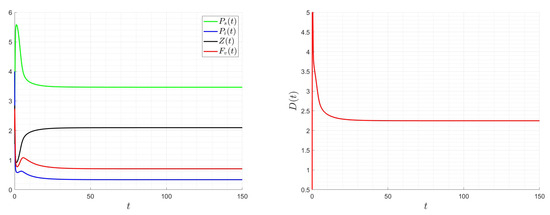
Figure 15. Impact of the optimal dilution rate on the system for ${\alpha }_1=1$, ${\alpha }_2=10$, and ${\alpha }_3=1$.

7. Conclusions

We looked at a straightforward mathematical model in four dimensions that describes the growth of zooplankton on phytoplankton that it are affected by a free virus under perfect mixing conditions in a chemostat. The phytoplankton were present in two forms: susceptible and infected phytoplankton. We studied the system by calculating the basic reproduction number, the steady states, and their local and global stability. We studied the sensitivity of the basic reproduction number with respect to the model’s parameters. Furthermore, we proposed an optimal control for the dilution rate with the aim to adjust the zooplankton concentration to an optimal value and decrease the virus concentration inside the bioreactor with optimal dilution costs. Lastly, we presented a number of numerical tests that validated the results.

The marine ecosystem may be at risk due to pollutants. Although there are many diverse sources of pollution, the most well-known ones include runoff from agriculture, industry, and home sewage. Plankton communities are impacted by environmental pollutants on a number of levels, including their abundance, growth methods, dominance, and succession patterns. These poisons are transferred cascadingly to higher trophic levels in the food chain during predation. The distribution pattern and behavioral characteristics of marine species in the ecosystems largely determine the rate of contact between environmental toxins and these organisms [54]. Among a variety of phytoplankton populations, environmental pollutants implicitly inhibit the proliferation of phytoplankton cells [55,56]. This growth inhibition tendency of environmental toxins has been statistically included in a few recent studies [41,42]. It has been demonstrated that a destabilized system can result from the growth inhibition of phytoplankton populations caused by environmental toxins. Therefore, removing environmental pollutants from an aquatic system is essential to keeping it stable. By taking into account toxin-producing phytoplankton and Markov switching in an intensively polluted environment, Yu et al. [43] investigated a stochastic phytoplankton–zooplankton model and discovered that the exogenous toxicant input and environmental fluctuations significantly impact plankton survival. Therefore, future research could look into the effects of both free viruses and environmental toxins on the growth of zooplankton on phytoplankton in a chemostat as a potential extension of this study.

References

- Lafferty, K.D.; Morris, A.K. Altered Behavior of Parasitized Killifish Increases Susceptibility to Predation by Bird Final Hosts. Ecology 1996, 77, 1390–1397. [Google Scholar] [CrossRef]
- Brooks, J.L.; Dodson, S.I. Predation, Body Size, and Composition of Plankton. Science 1965, 150, 28–35. [Google Scholar] [CrossRef] [PubMed]
- Leibold, W. Biodiversity and nutrient enrichment in pond plankton communities. Evol. Ecol. Res. 1999, 1, 73–95. [Google Scholar]
- DeMott, W. Optimal foraging theory as a predictor of chemically mediated food selection by suspension-feeding copepods. Limnol. Oceanogr. 1989, 34, 140–154. [Google Scholar]
- Mitra, A.; Castellani, C.; Gentleman, W.C.; Jonasdottir, S.H.; Flynn, K.J.; Bode, A.; Halsband, C.; Kuhn, P.; Licandro, P.; Agersted, M.D.; et al. Bridging the gap between marine biogeochemical and fisheries sciences; configuring the zooplankton link. Prog. Oceanogr. 2014, 129, 176–199. [Google Scholar] [CrossRef]
- De Troch, M.; Grego, M.; Chepurnov, V.A.; Vincx, M. Food patch size, food concentration and grazing efficiency of the harpacticoid Paramphiascella fulvofasciata (Crustacea, Copepoda). J. Exp. Mar. Biol. Ecol. 2007, 343, 210–216. [Google Scholar] [CrossRef]
- DeMott, W.R. Discrimination between algae and artificial particles by freshwater and marine copepods. Limnol. Oceanogr. 1988, 33, 397–408. [Google Scholar] [CrossRef]
- Pal, J.; Bhattacharya, S.; Chattopadhyay, J. Does predator go for size selection or preferential toxic-nontoxic species under limited resource? OJBS 2010, 10, 11–16. [Google Scholar]
- Aberle, N.; Hillebrand, H.; Grey, J.; Wiltshire, K.H. Selectivity and competitive interactions between two benthic invertebrate grazers (Asellus aquaticus and Potamopyrgus antipodarum): An experimental study using 13C-and 15N-labelled diatoms. Freshwater Biol. 2005, 50, 369–379. [Google Scholar] [CrossRef]
- Danielsdottir, M.G.; Brett, M.T.; Arhonditsis, G.B. Phytoplankton food quality control of planktonic food web processes. Hydrobiologia 2007, 589, 29–41. [Google Scholar]
- Huntley, M.; Sykes, P.; Rohan, S.; Marin, V. Chemically-mediated rejection of dinoflagellate prey by the copepods Calanus pacificus and Paracalanus parvus: Mechanism, occurrence and significance. Mar. Ecol. Prog. Ser. 1986, 28, 105–120. [Google Scholar] [CrossRef]
- Fulton, R.S., III; Paerl, H. Effects of colonial morphology on zooplankton utilization of algal resources during blue-green algal (Microcystis aeruginosa) blooms. Limnol. Oceanogr. 1987, 32, 634–644. [Google Scholar] [CrossRef]
- Paffenhofer, G.A.; Sant, K.B.V. The feeding response of a marine planktonic copepod to quantity and quality of particles. Mar. Ecol. Prog. Ser. 1985, 27, 55–65. [Google Scholar] [CrossRef]
- Evans, C.; Pond, D.W.; Wilson, W.H. Changes in Emiliania huxleyi fatty acid profiles during infection with E. huxleyi virus 86: Physiological and ecological implications. Aquat. Microb. Ecol. 2009, 55, 219–228. [Google Scholar] [CrossRef]
- Bratbak, G.; Egge, J.K.; Heldal, M. Viral mortality of the marine alga Emiliania huxleyi (Haptophyceae) and termination of algal blooms. Mar. Ecol. Prog. Ser. 1993, 93, 39–48. [Google Scholar] [CrossRef]
- Evans, C.; Wilson, W. Preferential grazing of Oxyrrhis marina on virus infected Emiliania huxleyi. Limnol. Oceanogr. 2008, 53, 2035–2040. [Google Scholar] [CrossRef]
- Vermont, A.; Martnez, J.M.; Waller, J.D.; Gilg, I.C.; Leavitt, A.H.; Floge, S.A.; Archer, S.D.; Wilson, W.H.; Fields, D.M. Virus infection of Emiliania huxleyi deters grazing by the copepod Acartia tonsa. J. Plankton Res. 2016, 38, 1194–1205. [Google Scholar] [CrossRef]
- Townsend, D.W.; Keller, M.D.; Holligan, P.M.; Ackleson, S.G.; Balch, W.M. Blooms of the coccolithophore Emiliania huxleyi with respect to hydrography in the Gulf of Maine. Cont. Shelf Res. 1994, 14, 979–1000. [Google Scholar] [CrossRef]
- Wilson, W.H.; Tarran, G.A.; Schroeder, D.; Cox, M.; Oke, J.; Malin, G. Isolation of viruses responsible for the demise of an Emiliania huxleyi bloom in the English Channel. J. Mar. Biol. Assoc. U. K. 2002, 82, 369–377. [Google Scholar] [CrossRef]
- Evans, C.; Kadner, S.V.; Darroch, L.J.; Wilson, W.H.; Liss, P.S.; Malin, G. The relative significance of viral lysis and microzooplankton grazing as pathways of dimethylsulfoniopropionate (DMSP) cleavage: An Emiliania huxleyi culture study. Limnol. Oceanogr. 2007, 52, 1036–1045. [Google Scholar] [CrossRef]
- Strom, S.; Wolfe, G.; Holmes, J.; Stecher, H.; Shimeneck, C.; Sarah, L. Chemical defense in the microplankton I: Feeding and growth rates of heterophic protists on the DMS-producing phytoplankter Emiliania huxleyi. Limnol. Oceanogr. 2003, 48, 217–229. [Google Scholar] [CrossRef]
- Wolfe, G.V.; Steinke, M. Grazing-activated production of dimethyl sulfide (DMS) by two clones of Emiliania huxleyi. Limnol. Oceanogr. 1996, 41, 1151–1160. [Google Scholar] [CrossRef]
- Steinke, M.; Malin, G.; Liss, P.S. rophic interaction in the sea: An ecological role for climate relevant volatiles? J. Phycol. 2002, 38, 630. [Google Scholar] [CrossRef]
- Beretta, E.; Kuang, Y. Modeling and analysis of a marine bacteriophage infection. Math. Biosci. 1998, 149, 57–76. [Google Scholar] [CrossRef] [PubMed]
- Beltrami, E.; Carroll, T. Modeling the role of viral disease in recurrent phytoplankton blooms. J. Math. Biol. 1994, 32, 857–863. [Google Scholar] [CrossRef]
- Gakkhar, S.; Negi, K. A mathematical model for viral infection in toxin producing phytoplankton and zooplankton system. Appl. Math. Comp. 2006, 179, 301–313. [Google Scholar] [CrossRef]
- Chattopadhyay, J.; Pal, S. Viral infection on phytoplankton-zooplankton system: A mathematical model. Ecol. Model. 2002, 151, 15–28. [Google Scholar] [CrossRef]
- Samanta, S.; Dhar, R.; Pal, J.; Chattopadhyay, J. Effect of enrichment on plankton dynamics where phytoplankton can be infected from free viruses. Nonlinear Stud. 2013, 20, 223–236. [Google Scholar]
- Bairagi, N.; Roy, P.K.; Sarkar, R.R.; Chattopadhyay, J. Virus replication factor may be a controlling agent for obtaining disease-free system in a multi-species eco-epidemiological system. J. Biol. Syst. 2005, 13, 245–259. [Google Scholar] [CrossRef]
- Bairagi, N.; Adak, D. Complex dynamics of a predator-prey-parasite system: An interplay among infection rate, predator’s reproductive gain and preference. Ecol. Compl. 2015, 22, 1–12. [Google Scholar] [CrossRef]
- Bairagi, N.; Saha, S.; Chaudhuri, S.; Dana, S.K. Zooplankton selectivity and nutritional value of phytoplankton influences a rich variety of dynamics in a plankton population model. Phy. Rev. E 2019, 99, 012406. [Google Scholar]
- Antweiler, R.C.; Patton, C.J.; Taylor, H.E. Nutrients. In Chemical Data for Water Samples Collected During Four Upriver Cruises on the Mississippi River Between New Orleans, Louisiana, and Minneapolis, Minnesota, May 1990–April 1992; Moody, J.A., Ed.; U.S. Geological Survey Open-File Report 94-523; U.S. Geological Survey: Reston, VA, USA, 1995; pp. 89–125. [Google Scholar]
- Bester, K.; Hhnerfuss, H.; Brockmann, U.; Rick, H.J. Biological effects of triazine herbicide contamination on marine phytoplankton. Arch. Environ. Contam. Toxicol. 1995, 29, 277–283. [Google Scholar]
- Rueter, J.R.; Chisholm, S.W.; Morel, F. Effects of copper toxicity on silicon acid uptake and growth in Thalassiosira pseudonana. J. Phycol. 1981, 17, 270–278. [Google Scholar]
- Biswas, S.; Tiwari, P.K.; Kang, Y.; Pal, S. Effects of zooplankton selectivity on phytoplankton in an ecosystem affected by free-viruses and environmental toxins. Math. Biosci. Eng. 2020, 17, 1272–1317. [Google Scholar] [CrossRef] [PubMed]
- Alsolami, A.A.; El Hajji, M. Mathematical Analysis of a Bacterial Competition in a Continuous Reactor in the Presence of a Virus. Mathematics 2023, 11, 883. [Google Scholar] [CrossRef]
- Albargi, A.H.; El Hajji, M. Bacterial Competition in the Presence of a Virus in a Chemostat. Mathematics 2023, 11, 3530. [Google Scholar] [CrossRef]
- El Hajji, M. Influence of the presence of a pathogen and leachate recirculation on a bacterial competition. Int. J. Biomath. 2024. Online ready. [Google Scholar] [CrossRef]
- El Hajji, M.; Al-Subhi, A.Y.; Alharbi, M.H. Mathematical investigation for two-bacteria competition in presence of a pathogen with leachate recirculation. Int. J. Anal. Appl. 2024, 22, 45. [Google Scholar] [CrossRef]
- Smith, H.L.; Waltman, P. The Theory of the Chemostat. Dynamics of Microbial Competition; Cambridge Studies in Mathematical Biology; Cambridge University Press: Cambridge, UK, 1995; Volume 13. [Google Scholar] [CrossRef]
- Rana, S.; Samanta, S.; Bhattacharya, S.; Al-Khaled, K.; Goswami, A.; Chattopadhyay, J. The effect of nanoparticles on plankton dynamics: A mathematical model. BioSystems 2015, 127, 28–41. [Google Scholar] [CrossRef]
- Panja, P.; Mondal, S.K.; Jana, D.K. Effects of toxicants on phytoplankton-zooplankton-fish dynamics and harvesting. Chaos Solit. Fract. 2017, 104, 389–399. [Google Scholar]
- Yu, X.; Yuan, S.; Zhang, T. Survival and ergodicity of a stochastic phytoplankton-zooplankton model with toxin-producing phytoplankton in an impulsive polluted environment. Appl. Math. Comp. 2019, 347, 249–264. [Google Scholar]
- Thieme, H.R. Convergence results and a Poincaré-Bendixson trichotomy for asymptotically autonomous differential equations. J. Math. Biol. 1992, 30, 755–763. [Google Scholar] [CrossRef]
- Sobieszek, S.; Wade, M.J.; Wolkowicz, G.S.K. Rich dynamics of a three-tiered anaerobic food-web in a chemostat with multiple substrate inflow. Math. Biosci. Eng. 2020, 17, 7045–7073. [Google Scholar] [CrossRef] [PubMed]
- Butler, G.J.; Freedman, H.I.; Waltman, P. Uniformly persistent systems. Proc. Am. Math. Soc. 1986, 96, 425–429. [Google Scholar]
- Butler, G.; Wolkowicz, G. Predator-mediated coexistence in a chemostat: Coexistence and competition reversal. Math. Model. 1987, 8, 781–785. [Google Scholar] [CrossRef][Green Version]
- Chitnis, N.; Hyman, J.; Cushing, J. Determining important parameters in the spread of malaria through the sensitivity analysis of a mathematical model. Bull. Math. Biol. 2008, 70, 1272–1296. [Google Scholar]
- Albargi, A.H.; El Hajji, M. Mathematical analysis of a two-tiered microbial food-web model for the anaerobic digestion process. Math. Biosci. Eng. 2023, 20, 6591–6611. [Google Scholar] [CrossRef]
- El Hajji, M. Mathematical modeling for anaerobic digestion under the influence of leachate recirculation. AIMS Math. 2023, 8, 30287–30312. [Google Scholar] [CrossRef]
- Fleming, W.; Rishel, R. Deterministic and Stochastic Optimal Control; Springer: New York, NY, USA, 1975. [Google Scholar] [CrossRef]
- Lenhart, S.; Workman, J.T. Optimal Control Applied to Biological Models; Chapman and Hall: Boca Raton, FL, USA, 2007. [Google Scholar] [CrossRef]
- Pontryagin, L.S.; Boltyanskii, V.G.; Gamkrelidze, R.V.; Mishchenko, E.F.; Trirogoff, K.N.; Neustadt, L.W. The Mathematical Theory of Optimal Processes; CRC Press: Boca Raton, FL, USA, 2000. [Google Scholar] [CrossRef]
- Labille, J.; Brant, J. Stability of nanoparticles in water. Nanomedicine 2010, 5, 985–998. [Google Scholar]
- Miao, A.J.; Schwehr, K.A.; Xu, C.; Zhang, S.J.; Luo, Z.; Quigg, A.; Santschi, P.H. The algal toxicity of silver engineered nanoparticles and detoxification by exopolymeric substances. Environ. Pollut. 2009, 157, 3034–3041. [Google Scholar] [CrossRef]
- Miller, R.J.; Bennett, S.; Keller, A.A.; Pease, S.; Lenihan, H. TiO2 nanoparticles are phototoxic to marine phytoplankton. PLoS ONE 2012, 7, e30321. [Google Scholar] [CrossRef] [PubMed]
Disclaimer/Publisher’s Note: The statements, opinions and data contained in all publications are solely those of the individual author(s) and contributor(s) and not of MDPI and/or the editor(s). MDPI and/or the editor(s) disclaim responsibility for any injury to people or property resulting from any ideas, methods, instructions or products referred to in the content. |
© 2025 by the authors. Licensee MDPI, Basel, Switzerland. This article is an open access article distributed under the terms and conditions of the Creative Commons Attribution (CC BY) license (https://creativecommons.org/licenses/by/4.0/).