Abstract
Sequential experimental designs enhance data collection efficiency by reducing resource usage and accelerating experimental objectives. This paper presents a model-driven approach to sequential Latin hypercube designs (SLHDs) tailored for second-order models. Unlike traditional model-free SLHDs, our method optimizes a conditional A-criterion to improve efficiency, particularly in higher dimensions. By relaxing the restriction of non-replicated points within equally spaced intervals, our approach maintains space-filling properties while allowing greater flexibility for model-specific optimization. Using Sobol sequences, the algorithm iteratively selects good points, enhancing conditional A-efficiency compared to distance minimization methods. Additional criteria, such as D-efficiency, further validate the generated design matrices, ensuring robust performance. The proposed approach demonstrates superior results, with detailed tables and graphs illustrating its advantages across applications in engineering, pharmacology, and manufacturing.
Keywords:
computer experiments; metamodel; Latin hypercube design; sequential design; sequential sampling; second-order model MSC:
62K05; 62K20
1. Introduction
The Design and Analysis of Computer Experiments (DACE) framework is essential for reducing computational costs in complex and resource-intensive simulations. At its core, metamodeling, or surrogate modeling, approximates the relationships between inputs and outputs, facilitating system evaluation, performance analysis, and decision-making across various industries. These metamodeling approaches can be broadly categorized into adaptive methods, which adjust as data are collected, and fixed-design methods, which rely on predefined experimental designs [1]. Sequential experimental designs play a crucial role in real-world applications where data collection is resource-intensive and costly. In engineering, these designs are widely used in aerodynamic simulations to optimize aircraft wing configurations while minimizing computational expenses. Kriging-based response surface methods, such as the Efficient Global Optimization (EGO) approach proposed in [2], provide efficient optimization strategies by balancing exploration and exploitation to reduce the number of required function evaluations. In manufacturing, sequential designs enhance material testing efficiency by identifying suitable production parameters with minimal waste, such as in semiconductor manufacturing and additive manufacturing [3].
Adaptive and sequential experimental designs are also pivotal in healthcare, particularly in clinical trials, where they improve flexibility and efficiency. These designs allow for modifications based on accumulating data, leading to more ethical and cost-effective studies. For instance, group sequential designs enable interim analyses, allowing early trial termination for efficacy or futility, thereby conserving resources and protecting participants from ineffective treatments [4]. By incorporating such adaptive strategies, the healthcare industry can accelerate drug development, optimize therapeutic interventions, and improve patient outcomes.
Sequential experimental designs have gained increasing attention in modern computational fields such as machine learning and Bayesian optimization, where they play a crucial role in improving efficiency and reducing computational costs. In machine learning, sequential designs have been widely used for hyperparameter optimization, where selecting informative sampling points enhances model performance. In [5], it was demonstrated that adaptive sequential designs outperform traditional grid or random search methods by focusing on the most promising regions of the search space, thereby reducing the number of function evaluations required. This strategy has been further extended to deep learning models [6], where Bayesian-based sequential designs improve neural network tuning. Similarly, in reinforcement learning, sequential model-based optimization techniques have been effectively applied to automate hyperparameter selection, as shown in [7]. In Bayesian optimization, sequential experimental designs enhance the efficiency of acquisition functions, ensuring that new sampling points maximize information gain [8]. These methods are particularly valuable in optimizing expensive black-box functions, such as engineering simulations and real-world decision-making systems. In [9], batch Bayesian optimization was introduced via local penalization, demonstrating its effectiveness in reducing evaluation costs while maintaining an exploration–exploitation balance. Additionally, [10] highlighted the advantages of Bayesian optimization in high-dimensional applications, where sequential designs mitigate the challenges posed by noisy observations and irregular search spaces, making them particularly suitable for applications like drug discovery and industrial process optimization.
The integration of sequential designs into machine learning and Bayesian optimization underscores their importance in enhancing computational efficiency and model performance. By systematically selecting points based on prior knowledge, these methods provide a structured and adaptive approach to experimental design, further solidifying their role in modern data-driven research.
Foundational research on experimental designs, such as Box and Draper’s work on response surface methodology, underscores the importance of efficient designs in reducing resource demands while maintaining model fidelity [11]. Space-filling designs are crucial for building reliable metamodels, as they ensure that design points uniformly cover the design space. The Maximin Latin Hypercube Design (LHD), introduced in [12], exemplifies this approach. While LHDs with strong space-filling properties have been extensively developed, their computational cost can be prohibitive in high-dimensional applications. Sequential LHDs, which progressively add design points until a desired accuracy is achieved, address this challenge [13]. This paradigm shift aligns with advancements in sequential experimentation highlighted in the general statistical literature, such as [14], which emphasizes the iterative nature of data-driven model building.
To further enhance computational efficiency and space-filling performance, [15] introduced the Sequential Recursive Evolution Latin Hypercube Design (RELHD), which uses a permutation inheritance algorithm for large-sample applications.
Building on this foundation, this research introduces a novel sequential design strategy that expands upon previous foundational works, such as [16]. Our method begins with an optimized batch of initial points chosen from a Sobol sequence, ensuring sufficient design space coverage by prioritizing points with better minimum distances. Subsequent points are sequentially added using an iterative trace minimization method to enhance design efficiency and prediction accuracy. This approach addresses the limitations of prior models, such as those by [17], and leverages the benefits of real-time adjustments for improved efficiency and accuracy, as emphasized in [1,15].
Sequential design, often referred to as multi-stage design, is a cost-effective approach for computer experiments. It allows data collection to proceed in stages, where points are selected based on a set criterion until a specified accuracy is achieved [18,19,20,21]. Sequential Latin Hypercube Designs (SLHDs) further enhance each stage through recursive permutation evolution algorithms [15], balancing systematic space coverage with computational efficiency. This flexibility supports multi-level accuracy trials for complex simulations, thereby improving model precision and adaptability in understanding and optimizing intricate systems.
Metamodeling in simulations aims to identify influential input variables and understand their relationships with outputs, dynamically updating as new data arrive [15]. Common metamodeling techniques include neural networks, Gaussian processes, and polynomial response surface approximations [22]. These surrogate models provide efficient input–output approximations while offering ease of interpretation [23]. Second-order polynomial models, which include main effects, quadratic effects, and two-way interactions, are commonly used to represent response surfaces and reveal significant interactions. Ref. [24] highlighted the risks of misinterpreting factor relationships, emphasizing the importance of accurate models.
For complex simulations, a full quadratic second-order model is frequently used, capturing both individual effects and interactions:
This model includes constant, linear, quadratic, and interaction effects, along with a random error term , helping characterize input–output relationships in complex systems. The error term should have zero mean and a finite positive variance that is independent of . Here, Y is the response, represents the factors, denotes the coefficients, and is the error term. By incorporating all second-order terms, this model facilitates accurate estimation of curvilinear and interaction effects, addressing the need for enhanced model fidelity, as highlighted in [25]. Following their evaluation, a good design for factor screening should maintain relatively small terms in the alias matrices. Specifically, the alias matrices for the first-order model, associated with two-factor interactions and pure quadratic terms, should contain small values for the design to be considered effective. Although the designs generated in our paper can still be used as model-free designs, their evaluation under the second-order model is important for additional comparisons.
Optimal experimental design is a well-established area in statistical modeling, with significant contributions focusing on minimizing information matrix-based criteria such as the trace (A-optimality) or determinant (D-optimality). These methods have been extensively applied in fixed-sample scenarios to ensure statistical efficiency in parameter estimation and model fitting. For example, the authors in [26] explored A-optimal designs for additive quadratic mixture models, demonstrating how support points shift from barycenters as the number of mixture components increases. Their work highlights the utility of A-optimality in mixture experiments, where responses depend on the proportions of components, and the design space is constrained to a simplex. The equivalence theorem [27] underpins these designs, ensuring that A-optimal designs minimize the trace of the inverse information matrix within the specified constraints. While optimal designs for fixed-sample settings are well documented, extensions to sequential and adaptive frameworks remain an active area of research. In adaptive model-based designs [28], design points are iteratively updated based on the statistical model, incorporating parameter estimates and their uncertainties to optimize efficiency dynamically. Such designs often rely on criteria like A- or D-optimality, conditional on previously selected points, to improve estimation accuracy over successive stages. In contrast to traditional model-free space-filling approaches such as Latin Hypercube Designs (LHDs) or maximum distance criteria, our work integrates model-driven principles into sequential design construction. Specifically, we utilize Sobol sequences, known for their low-discrepancy properties, to generate candidate points that balance space-filling characteristics with statistical efficiency under a second-order model. While Sobol sequences align with model-free approaches by covering the design space uniformly, their use here is adapted to optimize conditional A-optimality, addressing prediction variance iteratively. The sequential nature of the proposed designs distinguishes them from fixed-sample A-optimal designs, such as those explored by [26]. Unlike fixed-sample designs, the proposed method sequentially updates design points to account for conditional trace minimization, introducing flexibility in real-time applications. While the methodology shares theoretical similarities with adaptive model-based designs [28], it incorporates space-filling properties that are less emphasized in traditional optimal designs.
This paper introduces a novel sequential design approach leveraging a second-order model, applicable to both low- and high-dimensional settings. Our method begins with an optimized initial design selection using a curated Sobol sequence, which minimizes the required number of runs for reliable coefficient estimation while ensuring comprehensive coverage of the design space. To further refine the design, we employ an iterative trace minimization method that sequentially adds new points, reducing trace conditional on previously chosen design points aiming to minimize prediction variance and enhance model robustness. This approach effectively captures complex relationships in high-dimensional spaces, making it a versatile and efficient solution for experimental design.
Designs are evaluated using alphabetical efficiency criteria, including A-, G-, and D-efficiencies, and compared with other sequential methods to identify the most efficient approach. To validate the results, we use JMP version 17.0 software to assess the top-performing designs based on these criteria and Prediction Variance Average. The Methodology Section provides a detailed description of the procedures and algorithms, while the Results Section presents and discusses the findings.
2. Methodology
This section outlines the methodology developed for constructing conditionally efficient sequential designs tailored to fit a full second-order model, where efficiency is assessed iteratively based on the current set of design points. This approach prioritizes model-based criteria, focusing on trace minimization, which quantifies the total variance in estimating model coefficients. A lower trace value indicates higher design efficiency, ensuring the accurate estimation of the model parameters.
For each design configuration, we compute both the trace and the determinant of the inverse of the information matrix for the second-order model. To ensure compatibility with second-order modeling requirements, the design matrix, initially defined over the range , is scaled to the interval . This transformation aligns the design with standard experimental design practices, enhancing interpretability and robustness.
The second-order model employed in this methodology captures essential components for analyzing complex systems, including main effects, interactions, and quadratic terms. These components allow the model to represent primary trends, combined factor effects, and nonlinear behaviors, offering valuable insights for optimization. However, as dimensionality increases, the complexity of the model also grows, necessitating careful planning to ensure feasible and informative experimental designs.
Our methodology integrates an initial set of points generated using Sobol sequences, followed by sequential refinement as outlined in Algorithm 1. Sobol sequences are chosen for their low-discrepancy properties and uniformity, which ensure comprehensive coverage of the design space. Compared to random or Latin hypercube sampling (LHS), Sobol sequences offer greater consistency and uniformity, particularly in high-dimensional applications. Their deterministic nature ensures replicability, as the sequence only requires the sample size to yield consistent results. While adapting Sobol sequences to non-uniform distributions can be challenging in multidimensional settings, they generally outperform alternative methods in terms of uniformity and reduced error.
The minimum number of initial runs, which forms the foundation for the sequential design, is determined using the following equation:
where k represents the number of factors (dimensions, variables). This equation ensures that all model parameters, including interactions and quadratic effects, can be estimated. For example, when , the minimum number of runs required is 6, and for , the minimum is 10.
2.1. Derivation and Justification of Equation (2)
Equation (2) is derived from the total number of estimable parameters in a full second-order model. This ensures that the design includes the minimum number of runs required for complete model estimation while preventing redundancy in design points.
A second-order model with k factors consists of the following:
- k main effects ();
- two-factor interaction terms (, where );
- k quadratic terms (, for );
- A constant intercept term.
By summing these components, the total number of parameters to be estimated is
This equation aligns with standard experimental design principles, ensuring all model parameters can be estimated while maintaining computational efficiency. It adheres to widely accepted methodologies in response surface modeling, as detailed in [29].
By integrating Sobol sequences for initial point generation and employing sequential refinement based on trace minimization, our approach ensures both statistical efficiency and comprehensive space coverage. The resulting designs are reproducible, with detailed implementation steps available upon request from the corresponding author.
2.2. Initial Point Selection
The initial points for the design are generated using Sobol sequences, widely regarded as superior among low-discrepancy sequences (LDSs). Several LDSs, including Halton, Faure, Sobol, and Niederreiter sequences, are well known in this domain, but Sobol sequences are particularly effective in practical applications. Studies such as [30,31,32,33] emphasize the advantages of Sobol sequences over other LDSs.
Sobol sequences are especially popular in fields like financial engineering, with [34] highlighting their effectiveness in Monte Carlo Methods. The construction of Sobol sequences adheres to three key principles outlined in [35]:
- Ensuring good uniformity of distribution as the number of points (N) increases toward infinity.
- Achieving good distribution even for relatively small initial point sets.
- Providing a computationally efficient generation algorithm.
The unique properties of Sobol sequences, determined by their direction numbers, enable reliable performance across various dimensions and applications. These sequences were selected for this methodology due to their ability to
- Uniformly cover the design space, promoting a more representative exploration.
- Provide replicability, ensuring consistency in practical applications and enhancing the reproducibility of results.
To determine the minimum number of initial points, Equation (2) ensures that the design is sufficiently informative. This deliberate choice contrasts with methods such as in [17], which do not leverage a structured initialization. Using Sobol sequences, the proposed approach provides a strong foundation with uniform design space coverage and improved model accuracy.
2.3. Sequential Design Optimization
Our sequential design strategy iteratively enhances the design by adding points that minimize the trace of the information matrix. This criterion improves efficiency and estimation accuracy, particularly for high-dimensional second-order models. The goal is to maximize statistical efficiency rather than focusing solely on geometric considerations such as point spacing. Optimality criteria, such as minimizing the generalized variance (determinant of the information matrix) or the total variance (trace of the information matrix), are employed. However, it is important to note that in real-world sequential designs with random stopping, the information matrix should account for averaging across potential stopping points. This requires incorporating , the error variance, which is typically estimated at multiple interim stages during the design process. Such estimation introduces additional randomness into the stopping rule and affects the criterion being minimized. While this study assumes a deterministic stopping criterion (e.g., a user-defined or a fixed maximum number of iterations), incorporating -based random stopping remains a topic for future work.
Sequential points are added iteratively based on the conditional trace minimization of the information matrix, leading to
- Improved parameter estimation accuracy for both main effects and interaction terms.
- The retention of robust space coverage, critical for sequential design effectiveness.
Unlike methods such as that in [17], which prioritize maximizing spacing between points, our trace-based strategy focuses on minimizing prediction variance. This refinement ensures that the added points provide maximum information gain while balancing trade-offs between coverage and statistical robustness.
The iterative optimization process is computationally efficient, allowing the method to scale effectively for higher-dimensional or more complex models. This makes the approach practical and robust for applications involving large design spaces.
2.4. Enhanced Robustness and Accuracy
By prioritizing trace minimization, our methodology provides a statistically robust framework for sequential design. This focus ensures higher accuracy in parameter estimation, even in high-dimensional scenarios. Additionally, the use of Sobol sequences for initialization enhances robustness by guaranteeing uniform coverage across the factor space.
2.5. Importance of the Quadratic Model
This methodology ensures the precise estimation of nonlinear effects, which are critical in second-order models. While statistical efficiency is the primary focus, incorporating space-filling properties enhances the design’s ability to comprehensively explore the design space and robustly predict higher-order interactions. This approach bridges traditional space-filling designs, typically used in non-parametric settings, with model-based optimal design principles tailored to the sequential framework.
2.6. Summary of Contributions
This methodology emphasizes several key improvements over existing approaches:
- The incorporation of Sobol sequences for structured and robust initial design generation.
- The sequential addition of points based on trace minimization to balance statistical efficiency and space-filling properties.
- The comprehensive integration of the full quadratic regression model for capturing all relevant effects in high-dimensional settings.
- Enhanced robustness and accuracy through a focus on statistical efficiency and uniform design coverage.
2.7. Comparison with Adaptive Model-Based Frameworks
Adaptive model-based designs, as extensively discussed in works like [28], focus on iteratively updating experimental designs based on interim estimates of model parameters. These designs dynamically optimize criteria such as A-optimality or D-optimality, leveraging the information matrix conditioned on the current data. A notable feature of adaptive designs is their ability to incorporate parameter uncertainty and estimation variance () into the optimization process, making them particularly effective in sequential or real-time experimental settings.
In contrast, the proposed Sobol sequence-based approach introduces a hybrid methodology that balances space-filling properties with statistical efficiency under the second-order model framework. While adaptive model-based designs often rely heavily on parameter estimates from prior stages, the proposed method minimizes the conditional trace of the information matrix without explicitly incorporating . This distinction allows the design to remain computationally simpler and robust to parameter misestimation at early stages.
Key differences between the two approaches include the following:
- Optimization Framework: Adaptive designs optimize the information matrix by incorporating uncertainty estimates (e.g., ), while the proposed method focuses on the deterministic optimization of the conditional trace.
- Space-Filling Properties: Traditional adaptive designs emphasize statistical efficiency but may neglect space-filling considerations, particularly in non-parametric settings. The proposed method explicitly integrates Sobol sequences to ensure adequate coverage of the design space
- Stopping Rules and Sample Size Determination: Adaptive designs often use stopping rules tied to parameter uncertainty, leading to variable sample sizes. The proposed method, however, employs a predetermined sample size, simplifying the design process while maintaining efficiency. The stopping criterion was chosen based on the following considerations:
- Balance Between Convergence and Computational Cost: A threshold of ensures that additional points contribute minimal improvement while avoiding excessive computational costs.
- Empirical Justification: Prior studies have demonstrated that values in this range provide an effective balance between early stopping and full convergence [36].
- Comparison with Adaptive Stopping Rules: Adaptive model-based designs often determine stopping dynamically based on parameter updates, which may introduce instability in early-stage experiments. In contrast, the proposed method ensures a stable sample size while maintaining a rigorous efficiency criterion.
Both approaches share the objective of improving experimental efficiency but cater to different practical needs. Adaptive designs excel in scenarios where parameter uncertainty plays a dominant role, such as high-dimensional or highly nonlinear models. Conversely, the Sobol-based sequential design offers a flexible alternative for studies emphasizing both space-filling and statistical efficiency, particularly under the second-order polynomial framework.
The current comparison against model-free designs, such as Latin Hypercube Designs, is appropriate given the space-filling emphasis of Sobol sequences. However, incorporating a broader discussion of adaptive model-based frameworks places the proposed methodology within a more comprehensive context and highlights its unique contributions to sequential design theory.
2.8. Design Efficiency and Evaluation
In this section, we provide the criteria we use to evaluate and compare the designs. The designs are evaluated using D-, G-, and A-efficiency criteria, as represented in Equations (3), (4), and (5), respectively. A design is superior if it shows higher efficiency metrics and lower average prediction variance, as given in Equation (6), thereby enhancing predictive accuracy and precision.
2.8.1. D-Optimality Criterion
D-optimality assesses design efficiency by minimizing the volume of the joint confidence region for regression coefficients:
where X is the model matrix, n the number of runs, and p the number of model terms.
2.8.2. G-Optimality Criterion
G-optimality minimizes the maximum prediction variance across the design space:
where over x in the design space.
2.8.3. A-Optimality Criterion
A-optimality minimizes the cumulative variance of regression coefficients:
2.8.4. Prediction Variance Average
The comparative prediction variance at a point is calculated as follows:
To evaluate the design’s overall predictive performance, the Prediction Variance Average is computed by sampling multiple points uniformly across the design space using Sobol sequences. The arithmetic mean of the comparative prediction variances across these points represents the Prediction Variance Average.
Lower Prediction Variance Average values indicate a design with improved predictive performance. Mathematically, it is expressed as follows:
where represents the ith point, is the prediction variance at , and is the error variance.
Before presenting the step-by-step process, we provide an overview of the sequential design methodology.
Algorithm 1 outlines the step-by-step process for constructing our sequential design. The algorithm consists of two main parts:
- Initial Selection Phase: A set of initial points is generated using Sobol sequences and optimized based on the design criterion.
- Sequential Phase: Additional points are iteratively added to improve the design’s efficiency while maintaining space-filling properties.
The stopping criterion ensures that the process terminates when the specified number of points is reached or when further improvements become negligible.
| Algorithm 1: Sequential design Algorithm |
|
3. Results
This section presents the results of our proposed approach. The designs generated using our method are displayed in tables, and their efficiencies are analyzed and compared in detail.
3.1. Sequential Design for the Second-Order Model Using Trace Criteria
Table 1 presents the best trace values obtained for the entire design, which includes both the initial and sequentially added runs. The first column of the table specifies the number of factors (dimensions) in the design, covering both low- and high-dimensional cases. The second column shows the initial minimum number of runs required to fit the full quadratic model (initial points). The third column lists the maximum number of points added to the design. Points were added sequentially, one at a time, and all relevant statistics for each sequential point were recorded.

Table 1.
Sequential designs with the best trace values identified using the proposed method (see Section 2). The table provides details on the initial number of points and the total number of points at the final stage, with an additional 100 points added to each design as an example. The trace values represent the best results achieved for each design after multiple iterations.
3.2. Comparison of Our Sequential Design with Other Sequential Designs
In this section, we compare our sequential design, developed for the second-order model, with two alternative types of sequential designs. A detailed comparison is provided for designs with two, three, four, and five factors, with varying numbers of sequential runs added one at a time. The comparison begins with seven runs, which is the minimum required to estimate all coefficients in the full second-order model with two factors.
The first type of sequential design used for comparison is the Fully Sequential Space-Filling (FSSF) approach, specifically the FSSF–forward-reflected algorithm (FSSF-Fr), as described in [17]. In this design, points are added incrementally, one at a time, to construct the design.
The second type is the Sequential Latin Hypercube Design (SLH), which incorporates space-filling and projective properties, as proposed in [13]. In SLH, a search algorithm determines the number of points to add at each stage to maintain the projective property. To ensure the space-filling property, the maximin criterion is applied to validate the design. An example of the points added for a two-factor design is shown in Table 2. At stage 0, the design starts with five initial points. Table 2 details the exact number of points added at each stage, which may vary depending on the initial design of five points in the matrix.
Table 2.
Procedure for Sequential Latin Hypercube Design (SLH) for 2 dimensions with 5 stages.
In Table 2, empty cells in the SLH design column indicate that no design of this type exists for the specified number of runs, making it impossible to assess its efficiency. The table compares sequential designs and their efficiencies across three different methods. The first two columns represent the number of factors and the number of runs at each stage, while the subsequent three columns display the calculated efficiencies for each design.
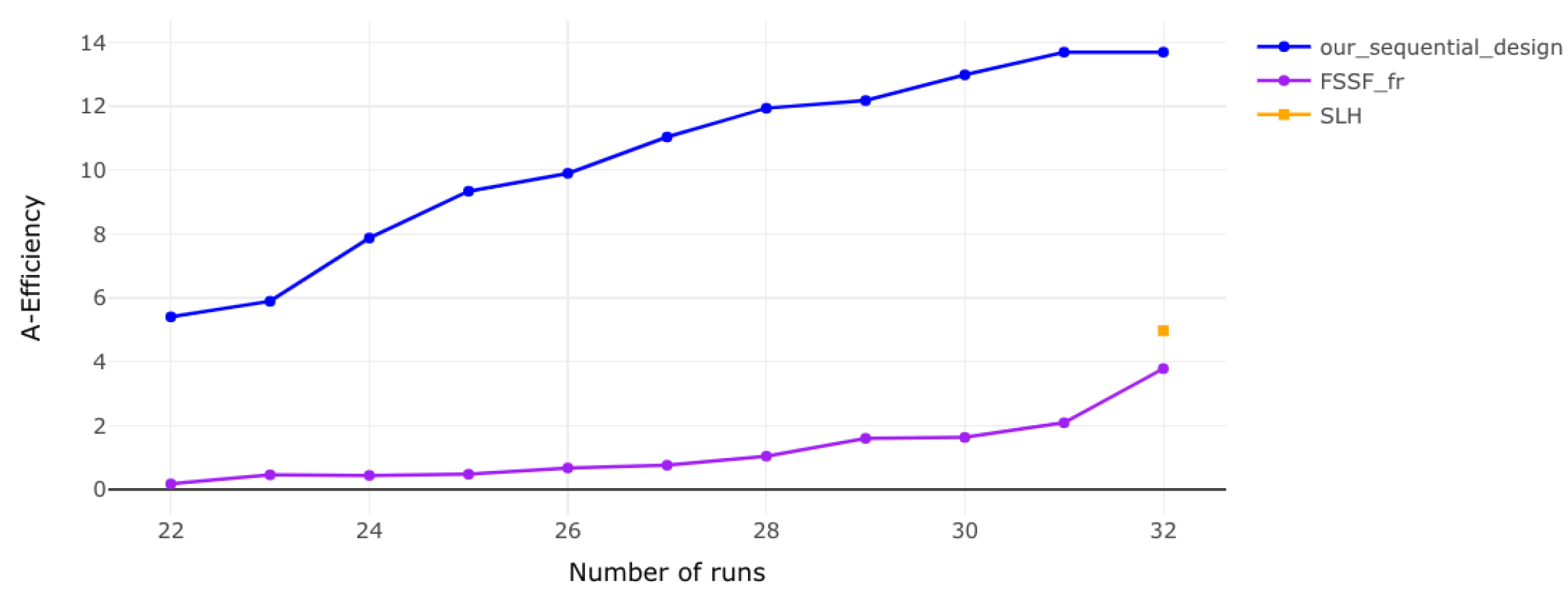
Table 3, Table 4, Table 5 and Table 6 and Figure 1, Figure 2, Figure 3 and Figure 4 illustrate that our sequential designs consistently achieve superior results, including higher efficiency and lower prediction variance, across all tested numbers of runs and factors. Across two- to five-factor experiments, our method outperforms the FSSF-Fr and SLH approaches in D-, G-, and A-efficiency, demonstrating improved parameter estimation, predictive accuracy, and robustness in high-dimensional settings. As the number of runs increases, the efficiency gap becomes more pronounced, particularly in G-efficiency, confirming the stability and reliability of our approach. Additionally, our designs achieve significantly lower Prediction Variance Average (Av), indicating more precise and consistent model predictions. Notably, our sequential designs outperform the FSSF designs in terms of A-efficiency.
Table 3.
Comparison between our sequential design and other sequential designs based on Efficiency and Prediction Variance Average for factors.
Table 4.
Comparison of our sequential design with other sequential designs based on Efficiency and Prediction Variance Average for factors.
Table 5.
Comparison of our sequential design with other sequential designs based on Efficiency and Prediction Variance Average for factors.
Table 6.
Comparison of our sequential design with other sequential designs based on Efficiency and Prediction Variance Average for factors.
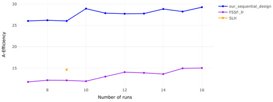
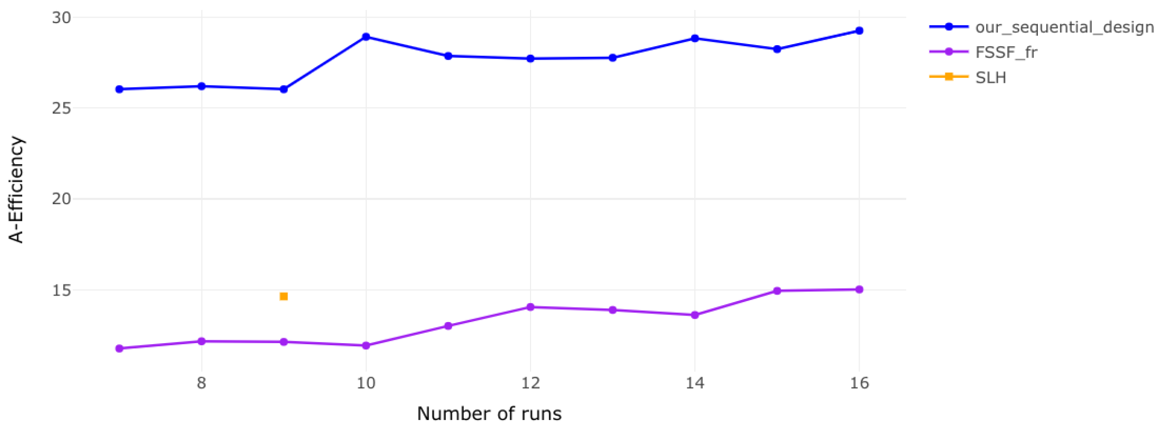
Figure 1.
A-efficiency for 2 factors. The results indicate that efficiency improves steadily as the number of runs increases, highlighting the benefits of additional runs for design performance.
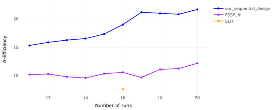
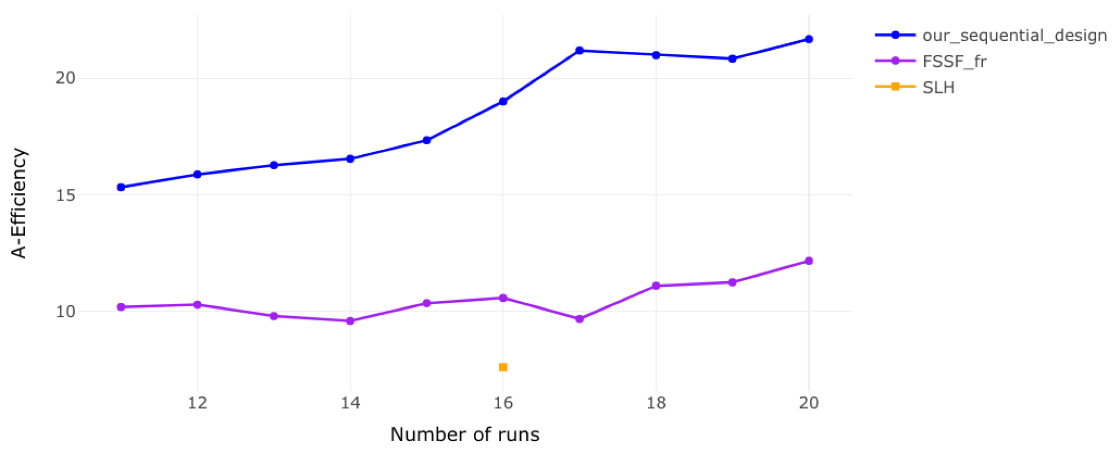
Figure 2.
A-efficiency for 3 factors. Similar to the 2-factor case, efficiency improves with more runs, but higher-dimensional designs show slightly lower initial efficiency before increasing.
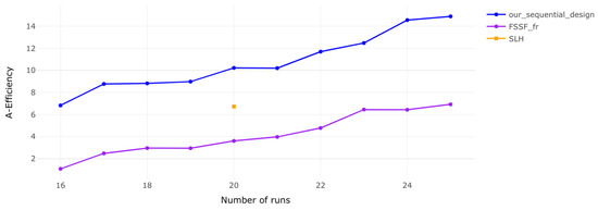
Figure 3.
A-efficiency for 4 factors. The efficiency trend continues, but higher-dimensional designs require more runs to reach comparable efficiency levels.

Figure 4.
A-efficiency for 5 factors. The efficiency remains lower at the beginning but improves as more runs are added, with diminishing returns highlighting the need for a balance between factors and runs.
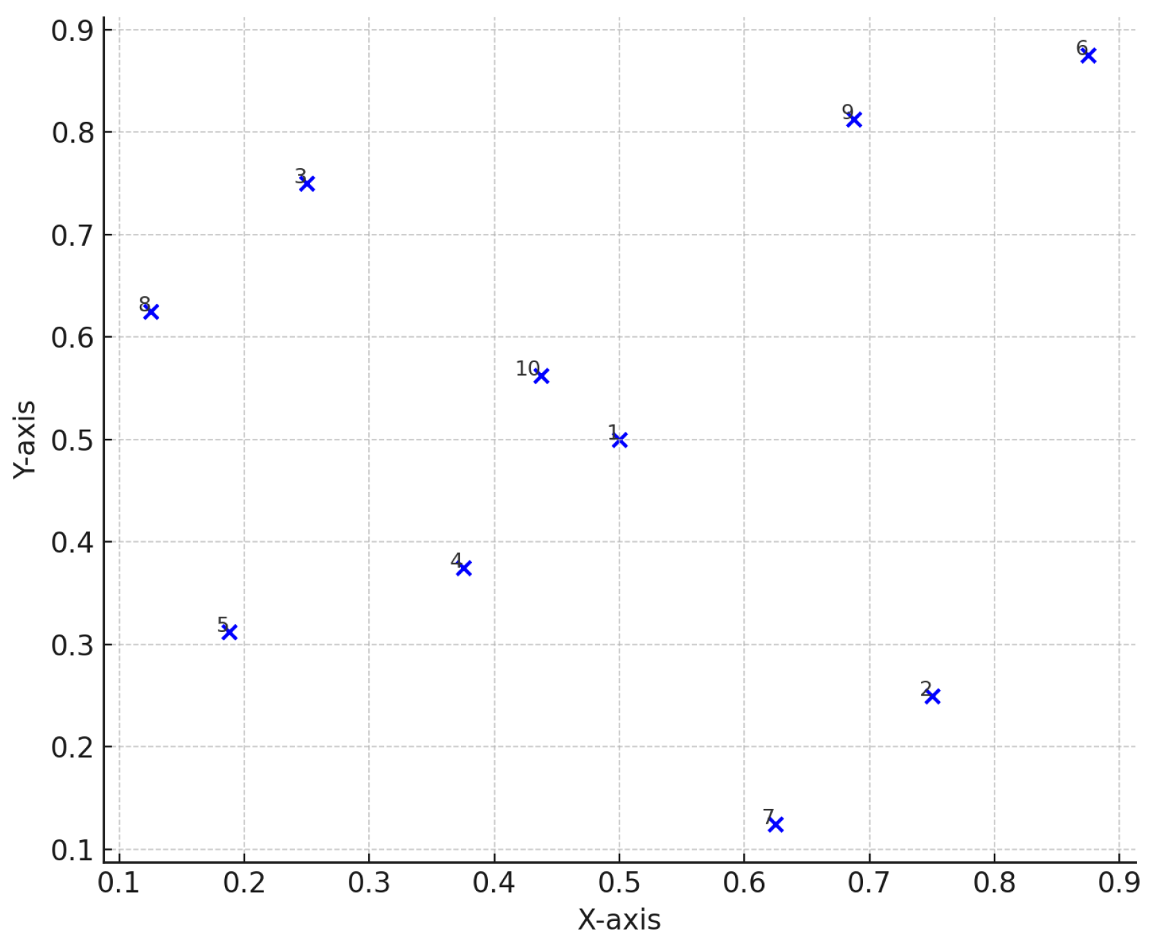
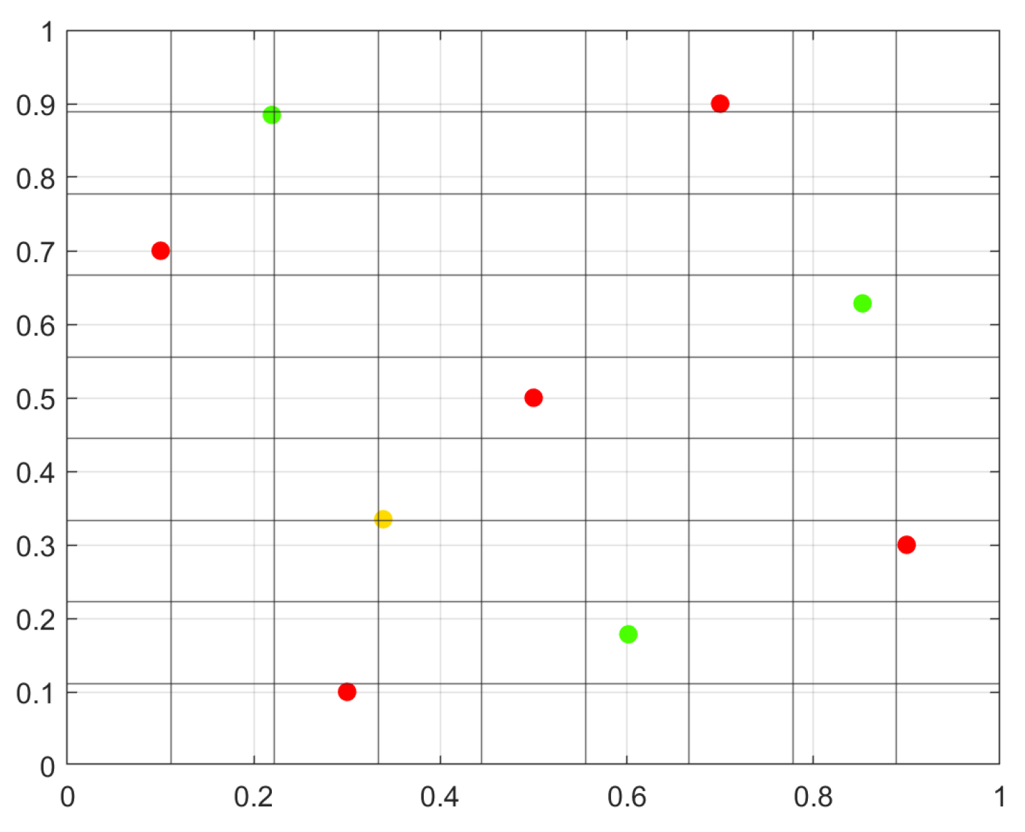
To further illustrate the sequential nature of the designs, Figure 5 presents an example of our proposed sequential design for a second-order model with two factors, where points are added sequentially based on the minimum trace criterion. For comparison, Figure 6 and Figure 7 show the corresponding FSSF-Fr and SLH designs, respectively. The FSSF-Fr design (Figure 6) follows the largest hole size criterion, sequentially adding new points in the largest empty region of the design space. Meanwhile, the SLH design (Figure 7) maintains the projective property by adding new points sequentially, determined using a search algorithm and the maximin criterion.
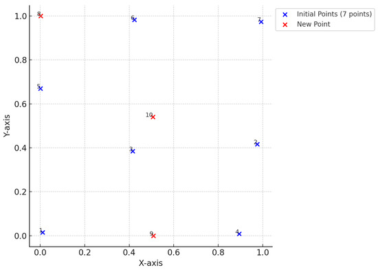
Figure 5.
Sequential design for a second-order model (2 factors). The design begins with 7 initial points, representing the minimum number of runs required to initiate the design. Additional points are added sequentially, one at a time, based on the minimum trace criterion.
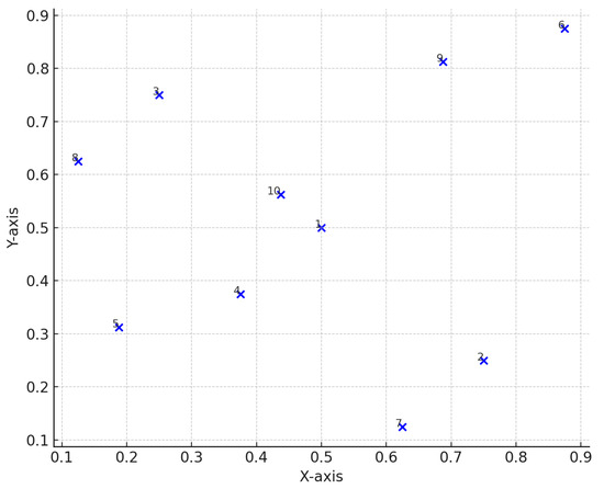
Figure 6.
FSSF-Fr Design (2 factors). This design starts without any points and sequentially adds them, one by one, using the largest hole size criterion to maximize space-filling properties. The points are numbered in the order they were added, clarifying the sequential process.
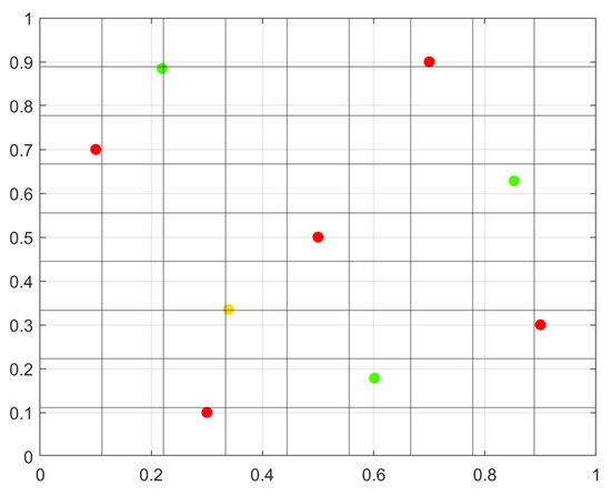
Figure 7.
SLH Design (2 factors). The design begins with 5 initial points (red) in the first stage. In the next stage, 1 new point (yellow) is added, followed by 3 additional points (green) in the final stage. A search algorithm determines the number of points to add at each stage to maintain the projective property. To ensure space-filling properties, the maximin criterion is applied.
Examples of sequential designs are provided in Appendix A, while the remaining designs are available upon request from the authors.
3.3. Correlations: Comparison of Designs with Two or Three Factors and 9 or 16 Runs
Summary of Comparison Between the Designs
The correlation analysis of model terms for designs with two and three factors demonstrates that Our Design consistently outperforms the SLH and FSSF sequential designs (see Table 7 and Table 8). Detailed observations are provided below.
Table 7.
Comparison of correlations for designs with 2 factors.
Table 8.
Comparison of correlations for 3 factors between designs.
Table 7 summarizes the results for designs with two factors. Compared to SLH and FSSF, Our Design consistently exhibits reduced correlations across main effects, two-factor interactions, and quadratic terms. By achieving lower correlations, Our Design minimizes multicollinearity, which is critical for ensuring precise and reliable model estimations. While FSSF can occasionally yield competitive results for correlations among main effects, its performance in high-dimensional models deteriorates due to increased correlations in more complex interactions.
Table 8 presents the results for designs with three factors. Our Design maintains lower correlations for two out of the three pairs of main effects when compared to the other two designs. As model complexity increases with the addition of a third factor, Our Design continues to exhibit lower correlations across more complex interactions. Notably, Our Design significantly improves the handling of second-order effects and cross-interactions. In contrast, SLH and FSSF exhibit moderate to high correlations, particularly in higher-order interactions, making them less effective for complex models.
In summary, Our Design consistently outperforms both SLH and FSSF by maintaining lower correlations, especially in scenarios where factor interactions are critical. This makes Our Design a viable choice for reducing multicollinearity and improving accuracy in high-dimensional, second-order models.
Comparison Based on Minimum Distance
The minimum pairwise distance, a critical metric for evaluating space-filling properties, indicates how evenly distributed the design points are. Higher minimum distance values suggest a more uniform spread, which is essential to prevent the clustering of points [17].
As shown in Table 9, our design consistently achieves a larger minimum pairwise distance compared to the FSSF_fr design across all factor and run configurations. For example,
- For two factors and nine runs, our design achieves a minimum distance of 0.3296, which is significantly better than FSSF_fr’s 0.1768.
- For three factors and 16 runs, our design performs better as well, with a minimum distance of 0.3226 compared to FSSF_fr’s 0.1036.
These results indicate that our designs excel in distributing points more evenly within the design space, thereby reducing the likelihood of clustering. Based on the minimum distance criterion, our designs offer superior space-filling properties, leading to a more uniform and efficient exploration of the design space.
Table 9.
Comparison of Our Design and FSSF_fr based on minimum distance.
Table 9.
Comparison of Our Design and FSSF_fr based on minimum distance.
| Factors | Number of Runs | Design | Minimum Distance |
|---|---|---|---|
| 2 | 9 | Our Design | 0.3296 |
| FSSF_fr | 0.1768 | ||
| 3 | 16 | Our Design | 0.3226 |
| FSSF_fr | 0.1036 | ||
| 4 | 20 | Our Design | 0.3227 |
| FSSF_fr | 0.1683 | ||
| 5 | 32 | Our Design | 0.3029 |
| FSSF_fr | 0.2306 |
3.4. Comparison of Design Methodologies and Performance Metrics
Unlike the methodology proposed in [17], which begins without predetermined points, our approach starts with a carefully selected set of initial points. This selection provides a strong foundation for model fitting, enabling more precise adjustments as model complexity increases. Our design approach leverages Sobol sequence points that minimize the trace, maximizing the information gained from each added point. This criterion contrasts with the spacing-focused strategy of [17], prioritizing trace minimization for more reliable and robust model fitting.
By integrating a quadratic regression model with a space-filling design, our approach effectively captures essential interaction and curvilinear effects, facilitating a thorough exploration of the design space for reliable parameter estimation. This makes our method particularly valuable in response surface methodologies that rely on the full second-order model.
In Table 10, we summarize the key characteristics of each design methodology. The first column of the table outlines the criteria used for comparison. We include the initial point selection criterion as it plays a crucial role in sequential experimentation. This criterion describes how the initial design points are chosen for each method. Different methods utilize varying numbers of initial design points, and the minimum number of runs presented in this table reflects the approach of each method.
Table 10.
Comparison of design methodologies and performance metrics.
The Sequential Refinement Strategy criterion characterizes the method employed during the sequential steps of the algorithms. The Correlation Performance criterion provides a qualitative assessment of the correlations among all terms in the full second-order model. For the Full Quadratic Model Efficiency criterion, we measure the adaptability of the generated design to accurately capture the effects of the full second-order model. Finally, the Coverage of Design Space criterion evaluates the uniformity of the design using the minimum distance between design points, as exemplified in Table 9.
4. Discussion
Sequential designs for the full quadratic model consistently deliver superior results across most stages. While there may be specific scenarios where sequential designs perform less optimally, they remain the preferred choice overall. This is because the point generation process can be stopped at any stage once the desired efficiency is achieved, making sequential designs highly cost-effective, particularly in high-dimensional applications. As demonstrated in Table 1, trace values systematically increase with the number of factors, reflecting the growing complexity of the full quadratic model while maintaining robust performance across all dimensions.
In high-dimensional settings with a large number of factors, such as 30 or 50, the full second-order model involves a substantial number of terms. For instance, with 30 factors, the minimum number of runs (initial points) required to estimate the full quadratic model is 597, necessitating the estimation of numerous parameters. Despite these challenges, our sequential designs maintain superior efficiency even in such complex cases.
Compared to other sequential designs, our approach consistently demonstrates greater efficiency, making it a practical and reliable choice for practitioners dealing with high-dimensional designs and demanding experimental requirements. To the best of our knowledge, this is the first study to develop high-dimensional sequential designs that are not only suitable but also highly efficient for the full second-order model, even when a large number of runs is required.
For example, in [13], Sequential Latin Hypercube Designs (SLHDs) are proposed that ensure even the coverage of the design space while maintaining projective properties at each stage for designs with up to five factors. This methodology begins with an initial random sample and incrementally adds points at each stage using a search algorithm guided by the “maximin” criterion. However, applying this approach to high-dimensional designs with a large number of runs becomes increasingly challenging due to difficulties in preserving the projective properties of Latin Hypercube Designs (LHDs) under such conditions.
Similarly, ref. [17] introduced fully sequential space-filling design algorithms for computer experiments, which start without any initial points and sequentially add points one at a time until the final stage. However, in our context, this approach requires an initial set of runs to meet the minimum number needed to estimate the second-order model. Only after this point can a fair comparison be made, where our designs demonstrate superior performance in terms of efficiency and robustness.
The proposed sequential design method consistently outperforms FSSF designs in terms of A-efficiency and predictive variance reduction; however, certain potential limitations and practical considerations may affect its effectiveness. One such factor is the presence of high noise levels in the response surface. The efficiency of the design relies on detecting underlying trends, but excessive noise or extreme irregularities can obscure these patterns, thereby limiting the benefits of sequential selection. In such cases, additional robustness measures may be necessary to maintain performance. Practical constraints also play a role, as real-world experimental settings often involve resource limitations such as time, budget, or material availability. The iterative nature of the sequential design process may pose logistical challenges, particularly in applications that require rapid decision-making.
Another consideration is the impact of high-dimensional settings. While the proposed approach remains efficient across various factor levels, its computational cost increases as the number of factors grows significantly. In cases where the number of factors becomes very large, space-filling properties and efficiency gains may plateau, suggesting that alternative criteria or hybrid approaches could be useful for maintaining performance. Despite these challenges, the method provides a systematic and effective framework for constructing sequential designs, particularly when experimental conditions support iterative refinement.
5. Conclusions
Sequential designs offer a highly flexible and efficient approach, as the number of runs can be minimized by halting the process once the desired efficiency is achieved. This eliminates the need to repeat all experiments whenever additional runs are required; instead, only the experiments corresponding to newly added points in the design need to be performed. This feature makes sequential designs particularly advantageous for high-dimensional spaces and a large numbers of factors.
Our proposed designs consistently outperform other sequential methods in terms of efficiency, demonstrating their practicality and robustness for high-dimensional applications. To the best of our knowledge, this work is the first to generate high-dimensional sequential designs that are both suitable and highly efficient for the full second-order model, even with a large number of runs.
For researchers and practitioners applying this methodology, several practical considerations should be taken into account. One key advantage is the flexibility to stop the sequential process at any stage, allowing researchers to balance efficiency with resource constraints. This adaptability enables practitioners to dynamically adjust the design based on experimental progress, optimizing the use of available resources while maintaining statistical rigor.
Scalability is another important factor, particularly for high-dimensional problems. Given the demonstrated robustness of this approach in handling multiple factors, it can be especially valuable in fields such as engineering, drug development, and machine learning, where high-dimensional experiments are common. The ability to construct efficient designs in such settings ensures that meaningful insights can be drawn from complex experimental data.
The integration of sequential designs with computational tools presents another promising direction. By incorporating optimization algorithms or surrogate modeling approaches, the implementation of these designs can be further streamlined, enhancing predictive accuracy and improving decision-making processes. Future research should focus on refining sequential design algorithms to preserve both space-filling and projective properties in high-dimensional settings. Additionally, exploring practical strategies for implementing these designs in real-world experimental scenarios would provide significant benefits to practitioners dealing with complex design challenges.
Author Contributions
Investigation, N.A.; methodology, N.A., S.G. and S.S.; software, N.A. and S.G.; supervision, S.G. and S.S.; writing—original draft preparation, N.A.; writing—review and editing, N.A., S.G. and S.S. All authors have read and agreed to the published version of the manuscript.
Funding
This research received no external funding.
Data Availability Statement
The datasets generated during the current study are available from the corresponding author upon reasonable request.
Acknowledgments
The authors thank the referees and the Associate Editor for their valuable comments and suggestions, which significantly improved the quality and presentation of this paper.
Conflicts of Interest
The authors declare no conflicts of interest.
Abbreviations
The following abbreviations and notations are used in this manuscript:
| ourD | Our sequential design for the second-order model |
| FSSF-Fr | Fully sequential space-filling (FSSF) design using the “forward-reflected” algorithm |
| SLH | Sequential Latin hypercube design with space-filling and projective properties |
| Tr | Trace |
| D | D-efficiency |
| G | G-efficiency |
| A | A-efficiency |
| Av | Prediction variance average |
Appendix A. Examples of Sequential Designs
Appendix A.1. Sequential Design of k = 2 Factors (7 to 16 Runs)
Table A1.
Sequential design of 2 factors (7 to 16 runs). Criteria values: D = 40.4946, G = 44.3569, A = 29.2564, Av = 0.2531.
Table A1.
Sequential design of 2 factors (7 to 16 runs). Criteria values: D = 40.4946, G = 44.3569, A = 29.2564, Av = 0.2531.
| Column 1 | Column 2 |
|---|---|
| 0.0108 | 0.0152 |
| 0.9754 | 0.4164 |
| 0.4151 | 0.3848 |
| 0.8936 | 0.0090 |
| 0.0006 | 0.6701 |
| 0.4230 | 0.9825 |
| 0.9927 | 0.9738 |
| 0.0014 | 0.9997 |
| 0.5083 | 0.0002 |
| 0.5065 | 0.5409 |
| 0.0012 | 0.0003 |
| 0.0001 | 0.5036 |
| 0.4927 | 0.9999 |
| 0.4824 | 0.5103 |
| 0.4965 | 0.0000 |
| 0.9993 | 0.0002 |
Appendix A.2. Sequential Design of k = 3 Factors (11 to 20 Runs)
Table A2.
Sequential design of 3 factors (11 to 20 runs). Criteria values: D = 33.10994, G = 25.42992, A = 21.67843, Av = 0.36401.
Table A2.
Sequential design of 3 factors (11 to 20 runs). Criteria values: D = 33.10994, G = 25.42992, A = 21.67843, Av = 0.36401.
| Column 1 | Column 2 | Column 3 |
|---|---|---|
| 0.9489 | 0.9298 | 0.5936 |
| 0.0151 | 0.0001 | 0.0776 |
| 0.0892 | 0.9842 | 0.0651 |
| 0.8926 | 0.0686 | 0.1197 |
| 0.6779 | 0.4855 | 0.9602 |
| 0.0412 | 0.1950 | 0.9496 |
| 0.9244 | 0.2111 | 0.6416 |
| 0.1992 | 0.8467 | 0.8846 |
| 0.6439 | 0.3801 | 0.0191 |
| 0.5442 | 0.0311 | 0.7962 |
| 0.3187 | 0.5808 | 0.5546 |
| 0.0001 | 0.5328 | 0.0067 |
| 0.6945 | 0.9953 | 0.9991 |
| 0.9982 | 0.4900 | 0.9980 |
| 0.0001 | 0.6379 | 0.5325 |
| 0.9986 | 0.9564 | 0.0005 |
| 0.0050 | 0.9995 | 0.9994 |
| 0.0021 | 0.0005 | 0.5435 |
| 0.4515 | 0.0020 | 0.0003 |
| 0.4779 | 0.9998 | 0.4399 |
Appendix A.3. Sequential Design of k = 4 Factors (16 to 25 Runs)
Table A3.
Sequential design of 4 factors (16 to 25 runs). Criteria values: D = 23.7704, G = 12.1565, A = 14.8842, Av = 0.5408.
Table A3.
Sequential design of 4 factors (16 to 25 runs). Criteria values: D = 23.7704, G = 12.1565, A = 14.8842, Av = 0.5408.
| Column 1 | Column 2 | Column 3 | Column 4 |
|---|---|---|---|
| 0.8004 | 0.3871 | 0.3372 | 0.0349 |
| 0.1255 | 0.9333 | 0.9888 | 0.7225 |
| 0.9516 | 0.0196 | 0.1142 | 0.0115 |
| 0.5548 | 0.4490 | 0.9549 | 0.3405 |
| 0.6455 | 0.1757 | 0.6861 | 0.8420 |
| 0.1669 | 0.7563 | 0.0716 | 0.3428 |
| 0.1050 | 0.6564 | 0.3664 | 0.2843 |
| 0.8708 | 0.1134 | 0.8523 | 0.2076 |
| 0.0706 | 0.4149 | 0.4083 | 0.9451 |
| 0.2837 | 0.9606 | 0.5904 | 0.0116 |
| 0.2314 | 0.8367 | 0.7542 | 0.9133 |
| 0.8532 | 0.7932 | 0.8145 | 0.9897 |
| 0.2844 | 0.0576 | 0.0967 | 0.6681 |
| 0.7382 | 0.4451 | 0.2149 | 0.7985 |
| 0.8651 | 0.9732 | 0.3895 | 0.2021 |
| 0.2993 | 0.1959 | 0.9788 | 0.2796 |
| 0.5513 | 0.0551 | 0.5319 | 0.1995 |
| 0.0189 | 0.0092 | 0.6084 | 0.2688 |
| 0.4063 | 0.6484 | 0.0056 | 0.0053 |
| 0.4293 | 0.9766 | 0.4356 | 0.9578 |
| 0.0022 | 0.0638 | 0.1707 | 0.0103 |
| 0.9590 | 0.3177 | 0.0621 | 0.9871 |
| 0.9544 | 0.9599 | 0.9748 | 0.0930 |
| 0.0359 | 0.0232 | 0.9690 | 0.9665 |
| 0.9942 | 0.3493 | 0.4295 | 0.6215 |
Appendix A.4. Sequential Design of k = 5 Factors (22 to 32 Runs)
Table A4.
Sequential design of 5 factors (22 to 32 runs). Criteria values: D = 21.72798, G = 9.786138, A = 13.69794, Av = 0.629681.
Table A4.
Sequential design of 5 factors (22 to 32 runs). Criteria values: D = 21.72798, G = 9.786138, A = 13.69794, Av = 0.629681.
| Column 1 | Column 2 | Column 3 | Column 4 | Column 5 |
|---|---|---|---|---|
| 0.8748 | 0.5675 | 0.8638 | 0.1398 | 0.7457 |
| 0.7481 | 0.1674 | 0.6136 | 0.1525 | 0.0277 |
| 0.7440 | 0.9465 | 0.4857 | 0.0025 | 0.2365 |
| 0.3875 | 0.4907 | 0.3941 | 0.5573 | 0.6313 |
| 0.6944 | 0.7744 | 0.0610 | 0.8966 | 0.3124 |
| 0.3858 | 0.4305 | 0.8007 | 0.7548 | 0.8426 |
| 0.0526 | 0.2489 | 0.7832 | 0.0739 | 0.1329 |
| 0.6378 | 0.0178 | 0.7259 | 0.2564 | 0.2116 |
| 0.9698 | 0.9390 | 0.8631 | 0.7861 | 0.4452 |
| 0.9903 | 0.0137 | 0.9355 | 0.2168 | 0.0161 |
| 0.1084 | 0.9368 | 0.2316 | 0.3529 | 0.0021 |
| 0.3458 | 0.0266 | 0.2470 | 0.0988 | 0.9192 |
| 0.1278 | 0.8349 | 0.8604 | 0.3570 | 0.2671 |
| 0.2885 | 0.2786 | 0.0172 | 0.3057 | 0.4591 |
| 0.8074 | 0.9914 | 0.3319 | 0.2039 | 0.0049 |
| 0.0350 | 0.2948 | 0.6154 | 0.6402 | 0.2384 |
| 0.6112 | 0.9439 | 0.7649 | 0.2982 | 0.8385 |
| 0.1549 | 0.9050 | 0.1829 | 0.1756 | 0.5494 |
| 0.8250 | 0.7717 | 0.2551 | 0.8276 | 0.8249 |
| 0.3101 | 0.6220 | 0.9147 | 0.3522 | 0.0173 |
| 0.3818 | 0.1804 | 0.1956 | 0.8054 | 0.9347 |
| 0.0644 | 0.6569 | 0.1245 | 0.9066 | 0.7698 |
| 0.3975 | 0.0300 | 0.0085 | 0.0036 | 0.0198 |
| 0.9796 | 0.3742 | 0.3730 | 0.9933 | 0.0001 |
| 0.4223 | 0.6049 | 0.9818 | 0.9948 | 0.1036 |
| 0.9854 | 0.0117 | 0.0182 | 0.1064 | 0.4049 |
| 0.0669 | 0.0066 | 0.0429 | 0.6708 | 0.0246 |
| 0.9877 | 0.7664 | 0.0187 | 0.2724 | 0.0030 |
| 0.9812 | 0.2880 | 0.9867 | 0.9948 | 0.8081 |
| 0.9926 | 0.6139 | 0.4161 | 0.2625 | 0.9905 |
| 0.0465 | 0.0014 | 0.9897 | 0.7405 | 0.1975 |
| 0.2719 | 0.9703 | 0.7564 | 0.9937 | 0.9939 |
References
- do Amaral, J.V.S.; Montevechi, J.A.B.; de Carvalho Miranda, R.; dos Santos, C.H. Adaptive Metamodeling Simulation Optimization: Insights, Challenges, and Perspectives. Appl. Soft Comput. 2024, 165, 112067. [Google Scholar]
- Jones, D.R.; Schonlau, M.; Welch, W.J. Efficient global optimization of expensive black-box functions. J. Glob. Optim. 1998, 13, 455–492. [Google Scholar] [CrossRef]
- Montgomery, D.C. Design and Analysis of Experiments; John Wiley & Sons: Hoboken, NJ, USA, 2017. [Google Scholar]
- Pallmann, P.; Bedding, A.W.; Choodari-Oskooei, B.; Dimairo, M.; Flight, L.; Hampson, L.V.; Holmes, J.; Mander, A.P.; Odondi, L.; Sydes, M.R.; et al. Adaptive designs in clinical trials: Why use them, and how to run and report them. BMC Med. 2018, 16, 29. [Google Scholar]
- Bergstra, J.; Bengio, Y. Random search for hyper-parameter optimization. J. Mach. Learn. Res. 2012, 13, 281–305. [Google Scholar]
- Snoek, J.; Larochelle, H.; Adams, R.P. Practical Bayesian optimization of machine learning algorithms. In Proceedings of the Advances in Neural Information Processing Systems 25 (NIPS 2012), Lake Tahoe, NV, USA, 3–6 December 2012; Volume 25. [Google Scholar]
- Hutter, F.; Hoos, H.H.; Leyton-Brown, K. Sequential model-based optimization for general algorithm configuration. In Proceedings of the International Conference on Learning and Intelligent Optimization, Rome, Italy, 17–21 January 2011; pp. 507–523. [Google Scholar]
- Frazier, P.I. A tutorial on Bayesian optimization. arXiv 2018, arXiv:1807.02811. [Google Scholar]
- Gonzalez, J.; Dai, Z.; Hennig, P.; Lawrence, N. Batch Bayesian optimization via local penalization. In Proceedings of the 19th International Conference on Artificial Intelligence and Statistics, San Diego, CA, USA, 9–12 May 2015; pp. 648–657. [Google Scholar]
- Shahriari, B.; Swersky, K.; Wang, Z.; Adams, R.P.; De Freitas, N. Taking the human out of the loop: A review of Bayesian optimization. Proc. IEEE 2016, 104, 148–175. [Google Scholar]
- Box, G.E.P.; Draper, N.R. Empirical Model-building and Response Surfaces; John Wiley & Sons: Hoboken, NJ, USA, 1987. [Google Scholar]
- Johnson, M.E.; Moore, L.M.; Ylvisaker, D. Minimax and maximin distance designs. J. Stat. Plan. Inference 1990, 26, 131–148. [Google Scholar] [CrossRef]
- Zhou, X.; Lin, D.K.; Hu, X.; Ouyang, L. Sequential Latin hypercube design with both space-filling and projective properties. Qual. Reliab. Eng. Int. 2019, 35, 1941–1951. [Google Scholar] [CrossRef]
- Wu, C.F.J.; Hamada, M. Experiments Planning Analysis and Parameter Design Optimization; John Wiley & Sons: Hoboken, NJ, USA, 2000. [Google Scholar]
- Li, G.; Yang, J.; Wu, Z.; Zhang, W.; Okolo, P.; Zhang, D. A sequential optimal Latin hypercube design method using an efficient recursive permutation evolution algorithm. Eng. Optim. 2024, 56, 179–198. [Google Scholar] [CrossRef]
- Lu, L.; Anderson-Cook, C.M. Strategies for building surrogate models in multi-fidelity computer experiments. J. Stat. Plan. Inference 2021, 215, 163–175. [Google Scholar]
- Shang, B.; Apley, D.W. Fully-sequential space-filling design algorithms for computer experiments. J. Qual. Technol. 2021, 53, 173–196. [Google Scholar] [CrossRef]
- Lam, C.Q. Sequential Adaptive Designs in Computer Experiments for Response Surface Model Fit. Ph.D. Thesis, The Ohio State University, Columbus, OH, USA, 2008. [Google Scholar]
- Loeppky, J.L.; Moore, L.M.; Williams, B.J. Batch sequential designs for computer experiments. J. Stat. Plan. Inference 2010, 140, 1452–1464. [Google Scholar] [CrossRef]
- Ranjan, P.; Bingham, D.; Michailidis, G. Sequential experiment design for contour estimation from complex computer codes. Technometrics 2008, 50, 527–541. [Google Scholar] [CrossRef]
- Williams, B.J. Sequential Design of Computer Experiments to Minimize Integrated Response Functions. Ph.D. Thesis, The Ohio State University, Columbus, OH, USA, 2000. [Google Scholar]
- Barton, R.R. Simulation metamodels. In Proceedings of the IEEE 1998 Winter Simulation Conference, Washington, DC, USA, 13–16 December 1998; Volume 1, pp. 167–174. [Google Scholar] [CrossRef]
- Vieira, H.; Sanchez, S.; Kienitz, K.H.; Belderrain, M.C.N. Generating and improving orthogonal designs by using mixed integer programming. Eur. J. Oper. Res. 2011, 215, 629–638. [Google Scholar] [CrossRef]
- Siggelkow, N. Misperceiving interactions among complements and substitutes: Organizational consequences. Manag. Sci. 2002, 48, 900–916. [Google Scholar] [CrossRef]
- Steinberg, D.M.; Lin, D.K.J. A Construction Method for Orthogonal Latin Hypercube Designs. Biometrika 2006, 93, 279–288. [Google Scholar]
- Chan, L.Y.; Guan, Y.N.; Zhang, C.Q. A-optimal designs for an additive quadratic mixture model. Stat. Sin. 1998, 8, 979–990. [Google Scholar]
- Kiefer, J. General equivalence theory for optimum designs (approximate theory). Ann. Stat. 1974, 2, 849–879. [Google Scholar]
- Fedorov, V.V.; Leonov, S.L. Optimal Design for Nonlinear Response Models; CRC Press: Boca Raton, FL, USA, 2013. [Google Scholar]
- Myers, R.H.; Montgomery, D.C.; Anderson-Cook, C.M. Response Surface Methodology: Process and Product Optimization Using Designed Experiments; John Wiley & Sons: Hoboken, NJ, USA, 2016. [Google Scholar]
- Paskov, S.; Traub, J.F. Faster Valuation of Financial Derivatives. J. Portf. Manag. 1996, 22, 113–123. [Google Scholar]
- Kreinin, A.; Merkoulovitch, L.; Rosen, D.; Zerbs, M. Measuring portfolio risk using quasi Monte Carlo methods. Algo Res. Q. 1998, 1, 17–26. [Google Scholar]
- Jäckel, P. Monte Carlo Methods in Finance; John Wiley & Sons: Hoboken, NJ, USA, 2002; Volume 5. [Google Scholar]
- L’Ecuyer, P.; Lemieux, C. Recent advances in randomized quasi-Monte Carlo methods. In Modeling Uncertainty: An Examination of Stochastic Theory, Methods, and Applications; Springer: New York, NY, USA, 2002; pp. 419–474. [Google Scholar]
- Glasserman, P. Monte Carlo Methods in Financial Engineering; Springer: New York, NY, USA, 2004. [Google Scholar]
- Sobol’, I.M. On the distribution of points in a cube and the approximate evaluation of integrals. Zhurnal Vychislitel’noi Mat. I Mat. Fiz. 1967, 7, 784–802. [Google Scholar]
- Nocedal, J.; Wright, S.J. Numerical Optimization, 2nd ed.; Springer: Berlin/Heidelberg, Germany, 2006. [Google Scholar] [CrossRef]


Disclaimer/Publisher’s Note: The statements, opinions and data contained in all publications are solely those of the individual author(s) and contributor(s) and not of MDPI and/or the editor(s). MDPI and/or the editor(s) disclaim responsibility for any injury to people or property resulting from any ideas, methods, instructions or products referred to in the content. |
© 2025 by the authors. Licensee MDPI, Basel, Switzerland. This article is an open access article distributed under the terms and conditions of the Creative Commons Attribution (CC BY) license (https://creativecommons.org/licenses/by/4.0/).