Novel Tensor Decomposition-Based Approach for Cell-Type Deconvolution in Visium Datasets with Reference scRNA-Seq Data Containing Multiple Minor Cell Types

Abstract

Conventional cell-type deconvolution methods, such as Robust Cell-Type Decomposition (RCTD), SPOTlight, Spatial Cellular Estimator for Tumors (SpaCET), and cell2location, often encounter limitations when applied to Visium datasets that include reference profiles with multiple minor cell types. This highlights the necessity for more advanced computational approaches to resolve such challenges. To address this issue, we have employed and refined tensor decomposition (TD)-based unsupervised feature extraction (FE) to integrate multiple Visium datasets, providing a robust platform for spatial gene expression profiling (spatial transcriptomics). Notably, TD-based unsupervised FE successfully retrieves singular value vectors that correspond with spatial distribution; neighboring spots are assigned vectors with comparable values. Additionally, TD-based unsupervised FE demonstrates successful interference of cell-type fractions within individual Visium spots, enabling effective deconvolution even when referencing single-cell RNA-seq datasets containing several minor cell types—a scenario where conventional methods, such as RCTD, SPOTlight, SpaCET, and cell2location, typically prove ineffective. The findings of this study suggest that TD-based unsupervised FE has broad applicability for diverse deconvolution tasks.

1. Introduction

Spatial transcriptomics enables spatial measurement of gene expression [1]. In particular, the 10x Genomics Visium platform facilitates the examination of tissue architecture by linking transcriptomic data to spatial context [2]. However, each Visium “spot” often contains gene expression signals from multiple cells [2], complicating the direct interpretation of cell-type composition [3]. Various computational deconvolution methods have emerged to resolve mixed spot-level signals into individual cellular components using single-cell RNA sequencing (scRNA-seq) references or other probabilistic and machine learning paradigms [3].

A key example is Robust Cell-Type Decomposition (RCTD), which employs a probabilistic framework to reliably assign cell-type identities to spots, modeling both biological and technical variability [4]. Meanwhile, SPOTlight adopts a seeded non-negative matrix factorization (NMF) regression strategy with scRNA-seq data, yielding interpretable spot-level spatial maps of cell-type distributions [5]. Spatial Cellular Estimator for Tumors (SpaCET) combines deconvolution with spatial autocorrelation analysis, characterizing local cell neighborhoods and potential interactions within tissue sections [6]. Meanwhile, cell2location uses a Bayesian approach to jointly model cell abundance and gene expression, inferring the spatial organization of fine-grained cell types across Visium spots [7].

Beyond these four primary applications, various methodologies have become integral to the spatial deconvolution toolkit. Stereoscope utilizes variational inference to reconcile scRNA-seq references with spatial transcriptomics data in a probabilistic manner, enabling the estimation of cell-type presence and abundance at each spot [8]. Tangram leverages deep learning to align high-dimensional single-cell RNA-seq profiles with Visium spots, facilitating inference of how distinct cell types and subtypes correspond to histological structures [9]. Furthermore, integrative pipelines within widely used bioinformatics platforms, such as Seurat [10,11,12] and Giotto [13], support spot deconvolution as well as downstream analyses, including trajectory inference and cell–cell interaction studies. Collectively, these approaches represent a dynamic and continuously evolving set of tools for examining cellular heterogeneity and spatial organization, providing unprecedented insights into tissue biology across healthy and disease states.

Despite their strengths, several existing tools are unable to effectively deconvolute Visium data when the reference single-cell gene expression contains multiple cell types. There are two types of single-cell gene expression reference datasets [14]: one for general application, which is not tailored to specific Visium data, and another that is customized for target Visium data. The latter is especially important in precision medicine, where the goal is to provide personalized treatment. Thus, although deconvolution is expected to yield precise results—particularly when the reference single-cell gene expression is associated with the target Visium dataset—this expectation does not hold true when the reference includes multiple minor cell types. Hence, a need exists for the development of advanced computational approaches capable of handling complex Visium datasets.

To address this issue, we propose a strategy utilizing TD-based unsupervised FE [15] to analyze Visium data. Here, a comparative analysis demonstrated the limitations of four conventional methods—RCTD, SPOTlight, SpaCET, and cell2location—when reference single-cell gene expression encompasses multiple minor cell types. Ultimately, these results establish our deconvolution strategy as a robust and effective approach for managing complex Visium datasets.

2. Materials and Methods

2.1. Visium

The Visium dataset [16] analyzed in this study was retrieved from GEO (GSE270382), comprising four Visium datasets, two of which were Tau-dKI, uninjected, while the others were Tau-dKI, injected. The data were obtained from the brain samples of mice with double-knockout AppNL-G-F/MAPT. The downloaded matrix files were loaded into R using the read.csv command and formatted as a sparse matrix using the spMatrix function in the Matrix package.

2.2. Single-Cell RNA-Seq and Annotated Cell Fraction Reference

Single-cell RNA-seq data [16] associated with the study Visium datasets were retrieved from GEO (GSE270385 and GSE270386). Two of the four datasets were obtained from GSE270385, and the remaining two from GSE270386 (GSM8341772 and GSM8341774). The .csv files were loaded into R using the read.csv command. The types of individual cells were inferred in the single-cell RNA-seq data using the SingleR function in SingleR [17]. Annotation was performed using the MouseRNAseqData() dataset in the celldex package [17]. The generated cell-type fractions are listed in Table 1.

Table 1. Fraction of cell-type annotation in reference single-cell gene expression associated with four Visium datasets ($1\le k\le 4$).

No.	k	1	2	3	4
1	Astrocytes	15	8	50	21
2	B cells	4	2	0	1
3	Epithelial cells	1	0	1	0
4	Fibroblasts	8	4	7	1
5	Macrophages	3	4	1	0
6	Microglia	3273	2950	1414	1697
7	Neurons	4638	3956	3987	4590
8	NK cells	2	1	1	0
9	Oligodendrocytes	6476	5365	3829	4274
10	T cells	30	16	39	11
11	Granulocytes	0	4	17	0
12	Monocytes	0	1	3	0
13	Dendritic cells	0	0	1	0
14	Endothelial cells	0	0	1	0

2.3. Detailed Setups and Parameters of Conventional Methods

In all cases, individual Visium datasets were analyzed separately, unlike TD-based unsupervised FE, which integrates four Visium datasets.

2.3.1. RCTD

Function create.RCTD was performed by max_cores = 2, CELL_MIN_INSTANCE = 1 to ensure that RCTD did not ignore minor cell types. Then, the function create.RUN was performed in the doublet_mode = ’multi’ to allow RCTD to attribute more than two cell types to individual spots.

2.3.2. SPOTlight

SPOTlight was performed with the default settings (see the source code provided in the Github link).

2.3.3. SpaCET

SpaCET was performed with the default settings (see the source code provided in the Github link).

2.3.4. Cell2location

Model learning was performed using the train function with max_epochs = 300, batch_size = 2500, train_size = 1, lr = 0.002, accelerator = “cpu”. Cell2location to initialize Visium data cell type annotation was performed with N_cells_per_location = 30, detection_alpha = 200. Then the train function was performed with max_epochs = 30,000, batch_size = adata_vis.n_obs, train_size = 1 (see the source code provided in the Github link).

2.4. TD-Based Unsupervised FE

Assume tensor as $x_{ijk}\in {\mathbb{R}}^{31053\times 4992\times 4}$, which represents the ith gene expression at the jth spot of the kth Visium dataset. Higher-order singular value decomposition [15] (HOSVD) was applied to $x_{ijk}$ to obtain

$$x_{ijk}=\sum _{{\ell }_1=1}^{31053}\sum _{{\ell }_2=1}^{4992}\sum _{{\ell }_3=1}^{4}G\left({\ell }_1{\ell }_2{\ell }_3\right)u_{{\ell }_{1}i}{u}_{{\ell }_{2}j}{u}_{{\ell }_{3}k}$$

(1)

where $G\in {\mathbb{R}}^{31053\times 4992\times 4}$ is a core tensor that represents the contribution of $u_{{\ell }_{1}i}{u}_{{\ell }_{2}j}{u}_{{\ell }_{3}k}$ toward $x_{ijk}$, $u_{{\ell }_{1}i}\in {\mathbb{R}}^{31053\times 31053}$, $u_{{\ell }_{2}j}\in {\mathbb{R}}^{4992\times 4992}$, $u_{{\ell }_{3}k}\in {\mathbb{R}}^{4\times 4}$, which are singular value matrices and orthogonal matrices.

HOSVD was performed by applying the irlba function in the irlba package to unfolded matrix $x_{i{j}^{\prime }}$ where $j^{\prime }=j+4992(k-1)$ as

$$x_{ijk}=x_{i{j}^{\prime }}\in {\mathbb{R}}^{31053\times 19968},(1\le k\le 4)$$

(2)

and we obtained

$$x_{i{j}^{\prime }}=\sum _{{\ell }_1}{\lambda }_{{\ell }_1}{u}_{{\ell }_{1}i}{v}_{{\ell }_1{j}^{\prime }}$$

(3)

HOSVD can be replaced by SVD on the unfolded matrix, since HOSVD simply applies SVD to the unfolded matrix.

Spots specifically contributing to the ℓth singular value vector, $u_{\ell i}$, were selected by attributing p-values to the ith gene by assuming that the null hypothesis $u_{\ell i}$ obeys Gaussian distribution,

$$P_i=P_{{\chi }^2}\left[>{\left({\displaystyle \frac{u_{{\ell }_{1}i}}{{\sigma }_{{\ell }_1}}}\right)}^2\right]$$

(4)

where $P_{{\chi }^2}\left[>x\right]$ is the cumulative ${\chi }^2$ distribution when the argument is larger than x and ${\sigma }_{{\ell }_1}$ is the standard deviation. The obtained p-values were corrected by the BH criterion, and the ith genes associated with adjusted p-values less than 0.01 were selected.

In the computation, ${\sigma }_{{\ell }_1}$ is optimized such that $u_{{\ell }_{1}i}$ obeys a Gaussian distribution when possible. The procedure is as follows: First, $P_i$ was computed assuming a degree of ${\sigma }_{{\ell }_1}$. Then, $P_i$s were corrected with the BH criterion, and ith genes associated with adjusted $P_i$ less than 0.01 were excluded. Next, the histogram of $P_i$ was computed for the non-excluded genes and the standard deviation of the histogram ${\sigma }_h$ was calculated as

$$\begin{array}{ccc}\hfill ⟨h_s⟩& =& {\displaystyle \frac{1}{S}}\sum _{s=1}^S{h}_s\hfill \end{array}$$

(5)

$$\begin{array}{ccc}\hfill {\sigma }_h& =& \sqrt{{\displaystyle \frac{1}{S}}\sum _{s=1}^S{\left(h_s-⟨h_s⟩\right)}^2}\hfill \end{array}$$

(6)

where $h_s$ is the histogram of $P_i$ at the sth bin and S is the total number of bins. We tune ${\sigma }_{{\ell }_1}$ so as to minimize ${\sigma }_h$.

${\sigma }_{{\ell }_1}$ was optimized because ${\sigma }_{{\ell }_1}$ should be the standard deviation of $u_{{\ell }_{1}i}$, thus obeying the null hypothesis; Gaussian ${\sigma }_{{\ell }_1}$ was computed using only non-excluded genes. The $u_{{\ell }_{1}i}$ values associated with smaller adjusted p-values were excluded because $u_{{\ell }_{1}i}$s associated with smaller adjusted p-values have larger absolute $u_{{\ell }_{1}i}$, causing ${\sigma }_{{\ell }_1}$ and $P_i$s to be overestimated. This would result in fewer selected genes. To circumvent this, we computed ${\sigma }_{{\ell }_1}$ using only non-excluded $u_{{\ell }_{1}i}$s.

2.5. Detailed Procedures

To clarify the methodology that led to the outcomes presented in figures in Section 3.4 and Section 4, we detail the step-by-step application of TD-based unsupervised FE to the Visium datasets (Figure 1). First, we applied TD-based unsupervised FE, obtaining $v_{{\ell }_1{j}^{\prime }}$, and plotted $v_{2j^{\prime }}$ on the spatial coordinate (Figure 2). Here the $j^{\prime }$th spots in $1\le j^{\prime }-4992(k-1)\le 4992$ belong to the kth Visium datasets. As nearby spots shared a similar abundance of $v_{2j}$, i.e., consistent with the spatial coordinate, we concluded that ${\ell }_2=2$ was the informative and variable component. Next, using $u_{2i}$ corresponding to $v_{2j}$, we attributed p-values to individual genes (is) and selected 277 genes to identify those with expression expected to be consistent with the spatial coordinate. We predicted that the 277 genes would align with the spatial coordinates and be biologically significant.

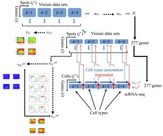
Figure 1. Four Visium datasets are integrated, generating $v_{{\ell }_1{j}^{\prime }}$, which is compared with the spatial coordinate. Given that $v_{2j^{\prime }}$ is consistent with the spatial coordinate, the corresponding $u_{2i}$ is used to select 277 genes with adjusted p-values less than 0.01. These genes are applied to compute $v_{{\ell }_1{j}^{\prime }}^{\mathrm{sel}}$ and $v_{1j^{\prime }}^{\mathrm{sel}}$ remains consistent with the spatial coordinate. Regression analysis is performed wherein $x_{i{j}^{\prime }}$ is fitted with $u_{{\ell }_{1}ik}^{\mathrm{sc}}$ and the spot-associated significant p-values are selected. p-values are related to $v_{4j^{\prime }}^{\mathrm{sel}}$. Finally, cell types of spots associated with significant adjusted p-values are inferred based on $v_{{\ell }_1{j}^{″}k}^{\mathrm{sc}}$. Red and blue arrows correspond to regression and cell type annotation, respectively.

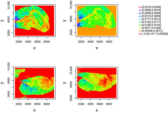
Figure 2. $v_{2j^{\prime }}$ attributed to the location of the $j^{\prime }$th spot. Top left: $k=1,1\le j^{\prime }\le 4992$. Top right: $k=2,4993\le j^{\prime }\le 9984$. Bottom left: $k=3,9985\le j^{\prime }\le 14,976$. Bottom right: $k=4$, $14,977\le j^{\prime }\le 19,968$.

2.6. Biological Interpretation

Subsequently, we sought to assess whether applying TD-based unsupervised FE to Visium data enables meaningful biological interpretation. This question remains unresolved, as each Visium spot encompasses multiple cells. In the absence of spot-specific annotations, concluding the outcomes proves challenging. One possible annotation for individual spots is the cell fraction, i.e., deconvolution. Fortunately, because we have associated the single-cell gene expression profile, spots could be annotated using single-cell RNA-seq. Hence, individual cells were annotated in single-cell RNA-seq datasets.

Next, we applied 277 genes as biomarker genes to relate gene expression in the individual spots to that of single-cell RNA-seq. We computed SVD, $u_{{\ell }_{1}ik}^{\mathrm{sc}}$, of single-cell RNA-seq using 277 genes. Linear regression

$$x_{i{j}^{\prime }}=x_{i[j^{\prime }-4992(k-1)]k}=a_{j^{\prime }0}+\sum _{{\ell }_1=1}^5{a}_{j^{\prime }{\ell }_1}{u}_{{\ell }_{1}ik}^{\mathrm{sc}}$$

(7)

was performed to determine if the expression of 277 genes in the Visium dataset could be represented by SVD computed from single-cell RNA-seq data where $a_{{\ell }_1{j}^{\prime }},1\le {\ell }_1\le 5$ are regression coefficients. Figure 3 shows the spatial distribution of $v_{1j^{\prime }}^{\mathrm{sel}}$ and the Spearman correlation coefficient between $x_{i{j}^{\prime }}$ and $a_{j^{\prime }0}+{\sum }_{{\ell }_1=1}^5{a}_{j^{\prime }{\ell }_1}{u}_{{\ell }_{1}ik}^{\mathrm{sc}}$, i.e., the left and right sides of Equation (7). Importantly, $v_{2j^{\prime }}^{\mathrm{sel}}$ does not exhibit consistency with the spatial coordinate, whereas $v_{1j^{\prime }}^{\mathrm{sel}}$ does.

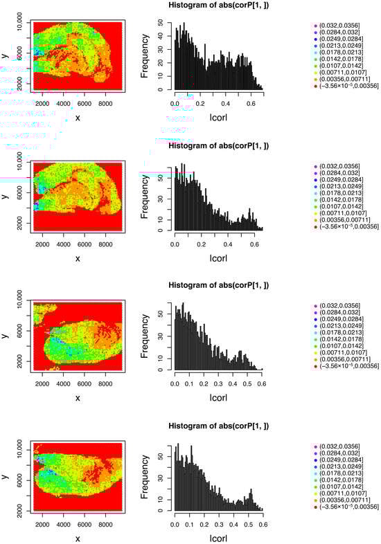
Figure 3. Left column: $v_{1j^{\prime }}^{\mathrm{sel}}$ attributed to the location of the $j^{\prime }$th spot. Right column: Spearman correlation coefficient histogram between $x_{i{j}^{\prime }}$ and $a_{j^{\prime }0}+{\sum }_{{\ell }_1=1}^5{a}_{j^{\prime }{\ell }_1}{u}_{{\ell }_{1}ik}^{\mathrm{sc}}$. First row: $k=1$, $1\le j^{\prime }\le 4992$; second row: $k=2,4993\le j^{\prime }\le 9984$; third row: $k=3,9985\le j^{\prime }\le 14,976$; fourth row: $k=4,14,977\le j^{\prime }\le 19,968$.

The results revealed that $v_{1j^{\prime }}^{\mathrm{sel}}$ remained consistent with the spatial coordinate, and $x_{i{j}^{\prime }}$ was computed efficiently from $u_{{\ell }_{1}ik}^{\mathrm{sc}}$. Table 2 presents the spot numbers with significant correlations between $x_{i{j}^{\prime }}$ and $a_{j^{\prime }0}+{\sum }_{{\ell }_1=1}^5{a}_{j^{\prime }{\ell }_1}{u}_{{\ell }_{1}ik}^{\mathrm{sc}}$.

Table 2. Number of spots with significant correlations.

	Adjusted p-Values
k	$>0.05$	$\le 0.05$
1	971	2076
2	1271	1769
3	1261	1349
4	1230	1351

The gene expression associated with most spots showed significant correlations with SVD computed from single RNA-seq data.

Additionally, we investigated the conditions under which spots showed significant correlation. To this end, we compute Spearman correlation coefficients between $v_{{\ell }_1{j}^{\prime }}^{\mathrm{sel}}$ and the negative-signed logarithmic p-values of linear regression. Results revealed that $v_{4j^{\prime }}^{\mathrm{sel}}$ exhibited the strongest correlation (Figure 4).

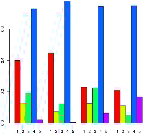
Figure 4. Absolute Spearman correlation coefficient between $v_{{\ell }_{1}j}^{\mathrm{sel}}$ and negative-signed logarithmic p-values of linear regression, Equation (7). Numbers below horizontal axis correspond to ${\ell }_1$. From the left to right, $k=1,2,3,4$.

Figure 5 shows the scatter plot between $v_{1j^{\prime }}^{\mathrm{sel}}$ and $v_{4j^{\prime }}^{\mathrm{sel}}$ where colors correspond to the absolute Spearman correlation coefficient between $x_{i{j}^{\prime }}$ and $a_{j^{\prime }0}+{\sum }_{{\ell }_1=1}^5{a}_{j^{\prime }{\ell }_1}{u}_{{\ell }_{1}ik}^{\mathrm{sc}}$ or negative-signed logarithmic p-values associated with the Spearman correlation coefficient.

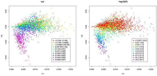
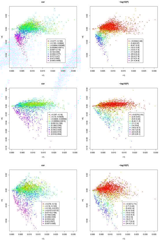
Figure 5. Scatter plot between $v_{1j^{\prime }}^{\mathrm{sel}}$ (horizontal axis) and $v_{4j^{\prime }}^{\mathrm{sel}}$ (vertical axis) where colors in the left column correspond to the absolute Spearman correlation coefficient between $x_{i{j}^{\prime }}$ and $a_{j^{\prime }0}+{\sum }_{{\ell }_1=1}^5{a}_{j^{\prime }{\ell }_1}{u}_{{\ell }_{1}ik}^{\mathrm{sc}}$; those in the right column are negative-signed logarithmic p-values associated with the Spearman correlation coefficient; first row: $k=1,1\le j^{\prime }\le 4992$; second row: $k=2,4993\le j^{\prime }\le 9984$; third row: $k=3,9985\le j^{\prime }\le 14,976$; fourth row: $k=4,14,977\le j^{\prime }\le 19,968$.

The larger negative $v_{4j^{\prime }}^{\mathrm{sel}}$ denoted a stronger inverse correlation. To determine whether $v_{4j^{\prime }}^{\mathrm{sel}}$ was still consistent with the spatial coordinate, $v_{4j^{\prime }}^{\mathrm{sel}}$ was applied to the spots (Figure 6).

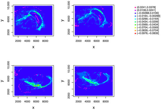
Figure 6. $v_{4j^{\prime }}^{\mathrm{sel}}$ attributed to the location of the $j^{\prime }$th spot. Top left: $k=1,1\le j^{\prime }\le 4992$. Top right: $k=2,4993\le j^{\prime }\le 9984$. Bottom left: $k=3,9985\le j^{\prime }\le 14,976$. Bottom right: $k=4$, $14,977\le j^{\prime }\le 19,968$.

The $v_{4j^{\prime }}^{\mathrm{sel}}$ remained consistent with the spatial coordinates.

We subsequently sought to associate the expression profiles of the 277 selected genes within individual spots, denoted as $x_{ijk}\in {\mathbb{R}}^{277\times 4992\times 4}$, with the singular value decomposition (SVD), $v_{{\ell }_1{j}^{″}k}^{\mathrm{sc}}$, derived from the reference single-cell RNA-seq data, also restricted to the same 277 genes as follows: the fraction of the sth cell type, $c_{j^{\prime }s}$, of the $j^{\prime }$th spot was computed as

$$\begin{array}{c}\hfill c_{j^{\prime }s}=a_{j^{\prime }0}+\sum _{{\ell }_1=1}^5\sum _{j^{″}=1}^{M_k}{a}_{j^{\prime }{\ell }_1}{v}_{{\ell }_1{j}^{″}k}^{\mathrm{sc}}{\delta }_{j^{″}s}\end{array}$$

(8)

where ${\delta }_{j^{″}s}$ takes 1 only when the $j^{″}$th cell in single-cell RNA-seq belongs to the sth cell type; otherwise, 0 is assigned. $M_k$ is the total number of single cells in the kth single-cell RNA-seq. $a_{j^{\prime }{\ell }_1}$s are those computed in Equation (7). $c_{j^{\prime }s}$ was computed only for spots associated with adjusted p-values less than 0.05 in Table 2. The associated results are presented in Figuers in Section 3.4 and Section 4.

2.7. A Brief Theoretical Explanation of the Robustness

The superior robustness of TD-based unsupervised FE compared to the other four approaches can be attributed to its unique ability to account for cell type proportion within single-cell reference profiles—a feature the others lack.

3. Results

3.1. Failure of Existing Methods

First, we sought to assess and compare the deconvolution performance of conventional methods (RCTD [4], SPOTlight [5], SpaCET [6] and cell2location [7]), when handling single-cell gene expression references that contain multiple minor cell types (Table 1). As observed, neurons, microglia, and oligodendrocytes formed the largest proportion of cells, consistent with the conclusion of a previous study [16]. Thus, the primary analysis focused on determining whether the deconvolution methods inferred these three cell types within the main cell populations. The results were then compared with those of TD-based unsupervised FE. Figure 7 illustrates this analysis.

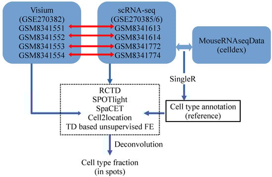
Figure 7. Study flow chart. Single-cell RNA-seq profiles are annotated using SingleR with the MouseRNAseqData reference from celldex. Annotated cell types and single-cell RNA-seq are used to deconvolute Visium datasets with RCTD, SPOTlight, SpaCET, cell2location, and TD-based unsupervised FE. Horizontal red arrows identify the correspondence between Visium datasets and reference single-cell RNA-seqs.

3.1.1. RCTD

To determine whether conventional methods can perform deconvolution successfully, even when the reference single-cell gene expression profile includes minor cell types, as shown in Table 1, we first tested RCTD [4], a SOTA that aims for deconvolution (Figure 8).

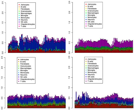
Figure 8. The first 100 cell populations for four Visium datasets ($1\le k\le 4$) provided by RCTD. Top left: $k=1$, top right: $k=2$, bottom left: $k=3$, bottom right: $k=4$.

Due to the complexity of cell deconvolution, which assigns multiple cell types to numerous individual spots, effectively displaying all results is challenging. Therefore, our initial visualizations focused on the first 100 spots in individual analyses, while broader patterns were subsequently explored through additional visual representations. The primary challenge for RCTD is that it detected numerous astrocytes that were reportedly absent in the original paper [16]. Hence, RCTD failed to effectively deconvolute the main cell types, likely because it did not account for cell populations in the reference single-cell gene expression. The RCTD model can be described as follows: suppose there are M spots, each measuring the expression of N genes. Then, $x_{ijk}$ is modeled by RCTD as

$$\begin{array}{ccc}\hfill x_{ijk}|{\lambda }_{ijk}& \sim & \mathrm{Poisson}\left(X_{jk}{\lambda }_{ijk}\right)\hfill \end{array}$$

(9)

$$\begin{array}{ccc}\hfill log\left({\lambda }_{ijk}\right)& =& {\alpha }_{jk}+log\left(\sum _{s=1}^{S_k}{\beta }_{jsk}{\mu }_{sik}+{\gamma }_{ik}+{ϵ}_{ijk}\right)\hfill \end{array}$$

(10)

where $X_{jk}$ is the total transcript count in the jth spot of the kth Visium dataset, $S_k$ is the number of cell types present in the kth Visium dataset, ${\alpha }_{jk}$ is a fixed spot-specific effect, ${\mu }_{sik}$ is the mean gene expression profile for cell type s and gene i, ${\beta }_{jsk}$ is the proportion of the contribution of cell type s to spot j, ${\gamma }_{ik}$ is a gene-specific platform random effect, and ${ϵ}_{ijk}$ is a random effect to account for other sources of variation, such as spatial effects. Given that RCTD does not consider cell populations in the reference, it cannot infer cell populations in individual Visium spots from those in the reference. This explains why RCTD erroneously counted astrocyte populations in individual spots, even though astrocytes were not present.

3.1.2. SPOTlight

Next, we employed SPOTlight [5] (Figure 9). As seen in Figure 9, for $k=2,3$, the cell proportion was excessively heterogeneous.

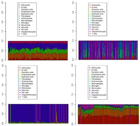
Figure 9. The first 100 cell populations for four Visium datasets ($1\le k\le 4$) provided by SPOTlight. Top left: $k=1$, top right: $k=2$, bottom left: $k=3$, bottom right: $k=4$.

The highly heterogeneous results may have been due to SPOTlight selecting marker genes before deconvolution. When possible, SPOTlight selects marker genes that are distinct across all cell types; this results in an unintended emphasis on minor cell types and unrealistic heterogeneous cell proportions. Thus, SPOTlight was also deemed to be unsuccessful.

3.1.3. SpaCET

Although SPOTlight and RCTD are SOTA, they represent older methodologies; as such, we evaluated SpaCET [6] as a newer alternative. Although SpaCET is primarily intended for tumor analysis, it can also handle other gene expression types if reference single-cell profiles associated with Visium data are available (Figure 10).

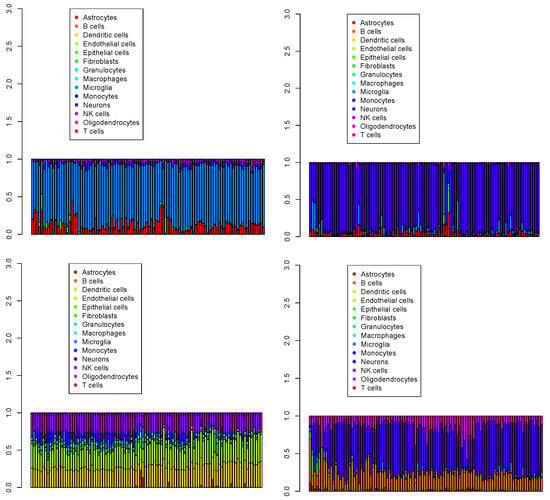
Figure 10. The first 100 cell populations for four Visium datasets ($1\le k\le 4$) provided by SpaCET. Top left: $k=1$, top right: $k=2$, bottom left: $k=3$, bottom right: $k=4$.

SpaCET failed to effectively process the data, as the four Visium datasets contained numerous cell types beyond the common neurons, microglia, and oligodendrocytes (see Table 1)—namely, astrocytes for $k=1$, dendritic cells, endothelial cells, and NK cells for $k=3$, and each Visium dataset comprised distinct cell fractions. More specifically, SpaCET considers only correlation coefficients of gene expression between individual single cells in the reference and Visium spots, thereby excluding cell-type fractions in the reference single-cell profiles, as was observed for RCTD.

3.1.4. Cell2location

Finally, we evaluated the performance of a more advanced Bayesian-based method, cell2location [7] (Figure 11).

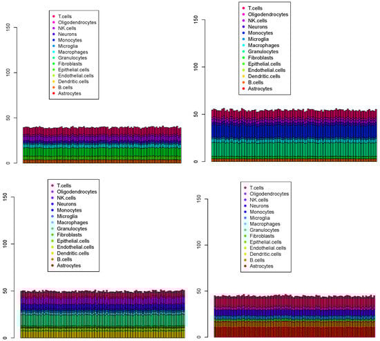
Figure 11. The first 100 cell population for four Visium datasets ($1\le k\le 4$) provided by cell2location. Top left: $k=1$, top right: $k=2$, bottom left: $k=3$, bottom right: $k=4$.

Although cell2location was predicted to offer higher accuracy and robustness than the other conventional methods, it is considerably time-consuming due to the need for direct probability optimization. Since none of the three predominant cell types identified in the four Visium datasets were neurons, microglia, or oligodendrocytes—the major types in the reference datasets (see Table 1)—the likelihood of cell2location achieving successful results was low. Moreover, cell2location requires a significantly longer runtime, spanning several days, while the other three methods complete in less than a few tens of minutes.

3.2. Overall Cell Type Fraction

While visualization restricted to the first 100 spots facilitated a rapid assessment of individual method performance, it did not provide sufficient information across all spots. To address this, we included pie charts showing the proportions of each identified cell type across all spots.

3.2.1. RCTD

As expected, Figure 8, RCTD erroneously identified astrocytes as a major cell type (see Table 1). Additionally, neurons were missing from one of the four pie charts, which should have represented a primary cell type (see Table 1), as seen in Figure 12. Thus, RCTD failed to predict the correct cell-type fractions.

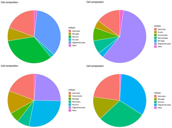
Figure 12. Pie charts of overall cell type fractions for four Visium datasets ($1\le k\le 4$) provided by RCTD. Top left: $k=1$, top right: $k=2$, bottom left: $k=3$, bottom right: $k=4$.

3.2.2. SPOTlight

As expected (Figure 10), four samples in Figure 13 were too distinct. For example, $k=3$ was dominated by neurons, whereas astrocytes predominated $k=4$. Meanwhile, highly distinct cell-type fractions are unlikely when considering the reference results (Table 1); thus, SPOTlight did not reproduce a reasonable cell-type fraction.

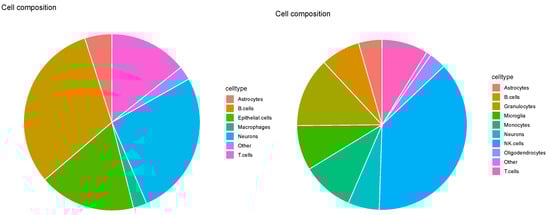
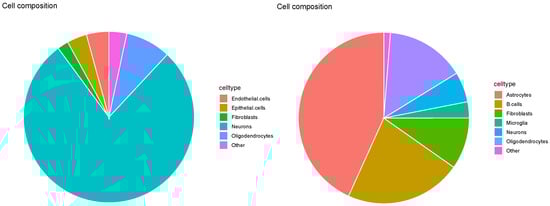
Figure 13. Pie charts of overall cell type fraction for four Visium datasets ($1\le k\le 4$) provided by SPOTlight. Top left: $k=1$, top right: $k=2$, bottom left: $k=3$, bottom right: $k=4$.

3.2.3. SpaCET

Evaluation of SpaCET based on the pie charts (Figure 14) revealed similar findings as those in Figure 10. That is, many cell types other than neurons, micoroglia, and oligodendrocytes, were identified, which did not accurately reflect the major cell types reported in the reference datasets (see Table 1). Given that these are major cell types in four Visium datasets (e.g., astrocytes for $k=1$, dendritic cells, endothelial cells, and NK cells for $k=3$), and that cell fractions estimated are too distinct between individual Visium datasets, SpaCET is hardly successful.

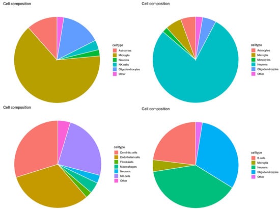
Figure 14. Pie charts of overall cell type fraction for four Visium datasets ($1\le k\le 4$) provided by SpaCET. Top left: $k=1$, top right: $k=2$, bottom left: $k=3$, bottom right: $k=4$.

3.2.4. Cell2location

Evaluation of SpaCET based on the pie charts (Figure 15) revealed results similar to those in Figure 11. In particular, none of the three major cell types identified in the four Visium datasets were neurons, microglia, or oligodendrocytes. Thus, cell2location was deemed insufficient for this task.

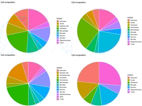
Figure 15. Pie charts of overall cell type fraction for four Visium datasets ($1\le k\le 4$) provided by cell2location. Top left: $k=1$, top right: $k=2$, bottom left: $k=3$, bottom right: $k=4$.

3.3. Spatial Abundance of Cell Types

Although the overall cell type fractions depicted in the pie charts provide sufficient evidence that these four methods are not effective—given that they have also identified non-existent cell types, as noted above—we present additional evidence of the limitations of these methods by analyzing the spatial abundance of cell types. In this analysis, we focus on three major reference cell types: microglia, neurons, and oligodendrocytes (Figure 16, Figure 17, Figure 18, Figure 19). The results clearly demonstrate that the four methods failed to achieve a reasonable spatial abundance, producing random abundances for all cell types. This further emphasized the limitations of these methods.

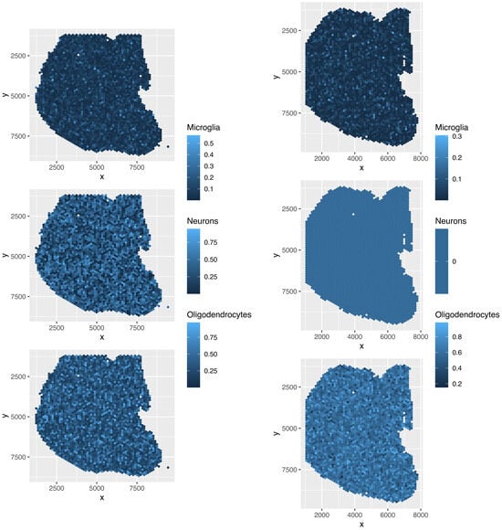
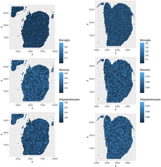
Figure 16. Spatial abundance of cell types for four Visium datasets ($1\le k\le 4$) provided by RCTD. Top left: $k=1$, top right: $k=2$, bottom left: $k=3$, bottom right: $k=4$.

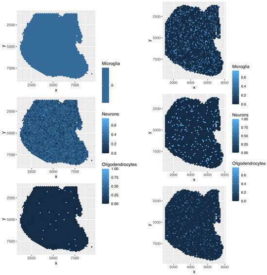
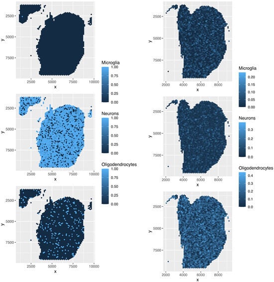
Figure 17. Spatial abundance of cell types for four Visium datasets ($1\le k\le 4$) provided by SPOTlight. Top left: $k=1$, top right: $k=2$, bottom left: $k=3$, bottom right: $k=4$.

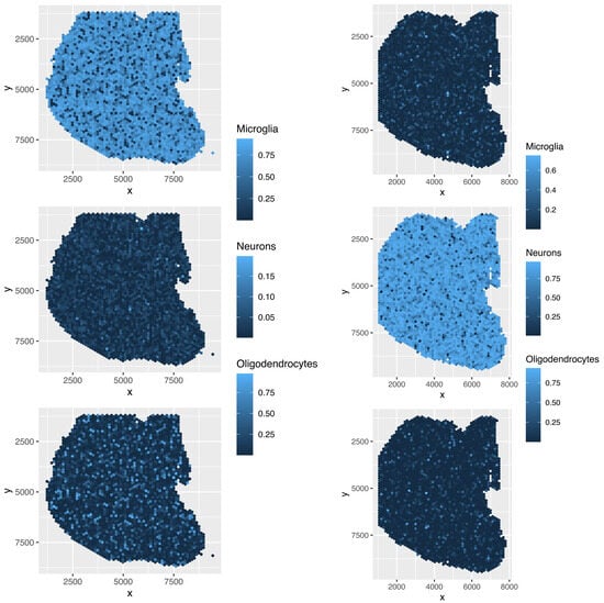
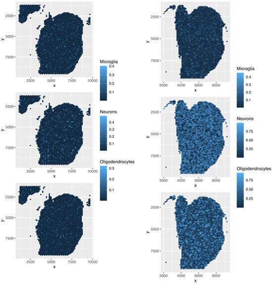
Figure 18. Spatial abundance of cell types for four Visium datasets ($1\le k\le 4$) provided by SpaCET. Top left: $k=1$, top right: $k=2$, bottom left: $k=3$, bottom right: $k=4$.

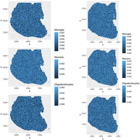
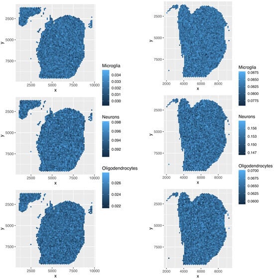
Figure 19. Spatial abundance of cell types for four Visium datasets ($1\le k\le 4$) provided by cell2location. Top left: $k=1$, top right: $k=2$, bottom left: $k=3$, bottom right: $k=4$.

3.4. TD-Based Unsupervised FE Applied to Visium Data

To determine whether TD-based unsupervised FE outperforms the other evaluated methods, we applied TD-based unsupervised FE to Visium data.

Figure 20 shows $c_{j^{\prime }s}$ cell-type profiles computed using TD-based unsupervised FE. For $1\le k\le 4$, the results show three primary cell types: microglia, neurons, and oligodendrocytes, with oligodendrocytes found to predominate. This aligned with the original study results [16]. Thus, the inference of cell types was reasonable, and TD-based unsupervised FE was determined to be the only method capable of successfully processing Visium datasets, even when the associated reference profiles included various minor cell types.

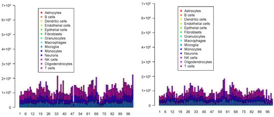
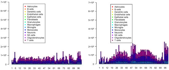
Figure 20. Pie charts of overall cell type fraction for four Visium datasets ($1\le k\le 4$) by TD-based unsupervised FE. Top left: $k=1$, top right: $k=2$, bottom left: $k=3$, bottom right: $k=4$.

4. Discussion

We also show the pie chart and spatial abundance of cell types (Figure 21 and Figure 22).

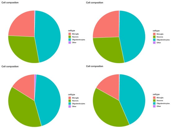
Figure 21. Pie charts of overall cell type fraction for four Visium datasets ($1\le k\le 4$) by-TD-based unsupervised FE. Top left: $k=1$, top right: $k=2$, bottom left: $k=3$, bottom right: $k=4$.

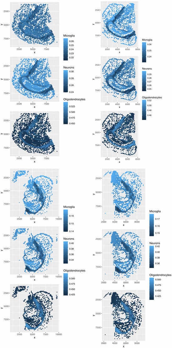
Figure 22. Spatial abundance of cell types for four Visium datasets ($1\le k\le 4$) by TD-based unsupervised FE. Top left: $k=1$, top right: $k=2$, bottom left: $k=3$, bottom right: $k=4$.

Various spots were missing in Figure 22 because only spots with gene expression that correlated with $u_{{\ell }_{1}ik}^{\mathrm{sc}}$ were plotted. The three major cell types replicated those reported in the reference (Table 1), and the spatial abundance was deemed reasonable. Hence, the TD-based unsupervised FE outperformed the other four methods.

While some may question our decision not to use a more established benchmark for evaluating the proposed method, our previous findings indicate that TD falls short of other state-of-the-art (SOTA) methods when tested on the standard benchmark [18]. Therefore, we assert that TD only outperforms SOTA in scenarios where the reference single-cell profiles contain numerous minor cell types. Additionally, we opted not to compare all the methods described in Section 1 because cell2location and RCTD are the top-performing methods [18]; assessing the remaining lower-ranking methods would require considerable time without providing further valuable insights.

TD-based unsupervised FE effectively reproduces spatial abundance (Figure 22) because it selects 277 genes based on the association between $v_{2j}$ and spatial abundance (Figure 2). Additionally, only the reference expression of genes, $u_{2i}$$u_{{\ell }_{1}ik}^{\mathrm{sc}}$, is used to estimate cell-type fractions, a step unique to TD-based unsupervised FE. Furthermore, by excluding spots that are unlikely to be predicted accurately Table 2, this method achieves higher prediction accuracy compared to the four other methods (Figure 22).

We selected the Visium dataset because conventional methods often fail to analyze it. Thus, we used TD-based unsupervised FE, demonstrating its effectiveness.

Based on our findings, none of the four methods showed clear advantages. Instead, they had notable disadvantages: inaccurate estimation of minor cell types—specifically, overestimating their abundance relative to single-cell profiles—and an inability to accurately predict the spatial abundance of cell types.

The computational running times for the methods evaluated in this study are as follows. RCTD is typically completed within 10 min, while SPOTlight requires more than 2 h. SpaCET generally finishes in approximately 20 min, whereas cell2loction may require days. Meanwhile, unsupervised FE based on TD can be completed within a few minutes.

Bioinformatics approaches focused on interaction prediction and network-based analysis may offer valuable insights for further discussion. Notable spatial cell–cell communication methods include CellChat [19], Giotto [20], and MISTy [21]. For graph neural network-based methodologies, SpaGCN [22] and STAGATE [23] are recommended. To bridge deconvolution with these techniques, NicheNet [24] and CARD [25] may be considered. Collectively, these resources contribute to a deeper understanding of the analytical landscape.

5. Conclusions

This paper shows that our TD-based unsupervised FE method can effectively deconvolute data, even when the single-cell reference profile contains several minor cell types—an area where four traditional techniques failed. We also suggest that identifying singular value vectors consistent with the spatial cell-type distribution may explain the success of this approach.

References

- Williams, C.G.; Lee, H.J.; Asatsuma, T.; Vento-Tormo, R.; Haque, A. An introduction to spatial transcriptomics for biomedical research. Genome Med. 2022, 14, 68. [Google Scholar] [CrossRef] [PubMed]
- Ståhl, P.L.; Salmén, F.; Vickovic, S.; Lundmark, A.; Navarro, J.F.; Magnusson, J.; Giacomello, S.; Asp, M.; Westholm, J.O.; Huss, M.; et al. Visualization and analysis of gene expression in tissue sections by spatial transcriptomics. Science 2016, 353, 78–82. [Google Scholar] [CrossRef] [PubMed]
- Li, B.; Dong, X.; Zhang, J.; Sui, T.; Colozo, J.M.; Ko, A.T.; Qiu, W.; Li, X.; Chang, A.; Ni, S.; et al. Benchmarking spatial and single-cell transcriptomics integration methods for transcript distribution prediction and cell type deconvolution. Nat. Methods 2022, 19, 662–670. [Google Scholar] [CrossRef] [PubMed]
- Cable, D.M.; Murray, E.; Zou, L.S.; Goeva, A.; Macosko, E.Z.; Chen, F.; Irizarry, R.A. Robust decomposition of cell type mixtures in spatial transcriptomics. Nat. Biotechnol. 2022, 40, 517–526. [Google Scholar] [CrossRef]
- Elosua-Bayes, M.; Nieto, P.; Mereu, E.; Gut, I.; Heyn, H. SPOTlight: Seeded NMF regression to deconvolute spatial transcriptomics spots with single-cell transcriptomes. Nucleic Acids Res. 2021, 49, e50. [Google Scholar] [CrossRef]
- Ru, B.; Huang, J.; Zhang, Y.; Aldape, K.; Jiang, P. Estimation of cell lineages in tumors from spatial transcriptomics data. Nat. Commun. 2023, 14, 568. [Google Scholar] [CrossRef]
- Kleshchevnikov, V.; Shmatko, A.; Dann, E.; Aivazidis, A.; King, H.W.; Li, T.; Elmentaite, R.; Lomakin, A.; Kedlian, V.; Gayoso, A.; et al. Cell2location maps fine-grained cell types in spatial transcriptomics. Nat. Biotechnol. 2022, 40, 661–671. [Google Scholar] [CrossRef]
- Andersson, A.; Bergenstråhle, J.; Asp, M.; Bergenstråhle, L.; Jurek, A.; Navarro, J.F.; Lundeberg, J. Single-cell and spatial transcriptomics enables probabilistic inference of cell type topography. Commun. Biol. 2020, 3, 565. [Google Scholar] [CrossRef]
- Biancalani, T.; Scalia, G.; Buffoni, L.; Avasthi, R.; Lu, Z.; Sanger, A.; Tokcan, N.; Vanderburg, C.R.; Segerstolpe, A.; Zhang, M.; et al. Deep learning and alignment of spatially resolved single-cell transcriptomes with Tangram. Nat. Methods 2021, 18, 1352–1362. [Google Scholar] [CrossRef]
- Satija, R.; Farrell, J.A.; Gennert, D.; Schier, A.F.; Regev, A. Spatial reconstruction of single-cell gene expression data. Nat. Biotechnol. 2015, 33, 495–502. [Google Scholar] [CrossRef]
- Stuart, T.; Butler, A.; Hoffman, P.; Hafemeister, C.; Papalexi, E.; Mauck, W.M., III; Hao, Y.; Stoeckius, M.; Smibert, P.; Satija, R. Comprehensive integration of single-cell data. Cell 2019, 177, 1888–1902.e21. [Google Scholar] [CrossRef]
- Hao, Y.; Hao, S.; Andersen-Nissen, E.; Mauck, W.M., III; Zheng, S.; Butler, A.; Lee, M.J.; Wilk, A.J.; Darby, C.; Zager, M.; et al. Integrated analysis of multimodal single-cell data. Cell 2021, 184, 3573–3587.e29. [Google Scholar] [CrossRef] [PubMed]
- Dries, R.; Zhu, Q.; Eng, C.H.L.; Li, R.; Liu, K.; Fu, Y.; Jiang, Z.; Ricker, A.; Barillas, D.; Correa de Sampaio, P.; et al. Giotto: A toolbox for integrative analysis and visualization of spatial expression data. Genome Biol. 2021, 22, 78. [Google Scholar] [CrossRef] [PubMed]
- Saqib, J.; Kim, J. From pixels to cell types: A comprehensive review of computational methods for spatial transcriptomics deconvolution. Genom. Inform. 2025, 23, 22. [Google Scholar] [CrossRef] [PubMed]
- Taguchi, Y.H. Unsupervised Feature Extraction Applied to Bioinformatics: A PCA Based and TD Based Approach, 2nd ed.; Unsupervised and Semi-Supervised Learning; Springer International Publishing: Cham, Switzland, 2024. [Google Scholar]
- Nagata, K.; Hashimoto, S.; Joho, D.; Fujioka, R.; Matsuba, Y.; Sekiguchi, M.; Mihira, N.; Motooka, D.; Liu, Y.C.; Okuzaki, D.; et al. Tau Accumulation Induces Microglial State Alterations in Alzheimer’s Disease Model Mice. eNeuro 2024, 11, ENEURO.0260-24.2024. [Google Scholar] [CrossRef]
- Aran, D.; Looney, A.P.; Liu, L.; Wu, E.; Fong, V.; Hsu, A.; Chak, S.; Naikawadi, R.P.; Wolters, P.J.; Abate, A.R.; et al. Reference-based analysis of lung single-cell sequencing reveals a transitional profibrotic macrophage. Nat. Immunol. 2019, 20, 163–172. [Google Scholar] [CrossRef]
- Sang-aram, C.; Browaeys, R.; Seurinck, R.; Saeys, Y. Spotless, a reproducible pipeline for benchmarking cell type deconvolution in spatial transcriptomics. eLife 2024, 12, RP88431. [Google Scholar] [CrossRef]
- Jin, S.; Guerrero-Juarez, C.F.; Zhang, L.; Chang, I.; Ramos, R.; Kuan, C.H.; Myung, P.; Plikus, M.V.; Nie, Q. Inference and analysis of cell-cell communication using single-cell and spatial transcriptomics data. Nat. Commun. 2021, 12, 1088. [Google Scholar] [CrossRef]
- Dries, R.; Zhu, Q.; Dong, R.; Eng, C.H.L.; Li, H.; Liu, K.; Fu, Y.; Zhao, T.; Sarkar, A.; Bao, F.; et al. Giotto: A spatial representation and visualization system for spatial transcriptomics data. Genome Biol. 2021, 22, 1–30. [Google Scholar] [CrossRef]
- Tanevski, J.; Nguyen, T.; Truong, B.; Sæz-Rodríguez, J. MISTy: An explainable multiview framework for intercellular signaling network modeling from spatial transcriptomics data. Genome Biol. 2022, 23, 1–26. [Google Scholar]
- Hu, J.; Li, X.; Coleman, K.; Schroeder, A.; Ma, N.; Xu, D.J.; Choi, Y.; Contributors, B.S.D.; Sheu, K.M.; Chen, P.; et al. SpaGCN: Integrating gene expression, spatial location and histology to identify spatial domains and spatially variable genes by graph convolutional network. Nat. Methods 2021, 18, 1342–1351. [Google Scholar] [CrossRef]
- Dong, K.; Zhang, S. Deciphering spatial domains from spatially resolved transcriptomics with an adaptive graph attention auto-encoder. Nat. Commun. 2022, 13, 1739. [Google Scholar] [CrossRef]
- Browaeys, R.; Saelens, W.; Saeys, Y. NicheNet: Modeling intercellular communication by linking ligands to target genes. Nat. Methods 2020, 17, 159–162. [Google Scholar] [CrossRef]
- Ma, Y.; Zhou, X. Spatially informed cell-type deconvolution for spatial transcriptomics. Nat. Biotechnol. 2024, 42, 1311–1321. [Google Scholar] [CrossRef]
Disclaimer/Publisher’s Note: The statements, opinions and data contained in all publications are solely those of the individual author(s) and contributor(s) and not of MDPI and/or the editor(s). MDPI and/or the editor(s) disclaim responsibility for any injury to people or property resulting from any ideas, methods, instructions or products referred to in the content. |
© 2025 by the authors. Licensee MDPI, Basel, Switzerland. This article is an open access article distributed under the terms and conditions of the Creative Commons Attribution (CC BY) license (https://creativecommons.org/licenses/by/4.0/).