Innovation-Adjusted Dynamics of E-Waste in the European Union: Mathematical Modeling, Stability and Panel EKC Turning Points

Abstract

The rapid growth of Waste Electrical and Electronic Equipment (WEEE) in the European Union highlights the need for a rigorous understanding of its long-term dynamics and the role of innovation in shaping its trajectory. This study investigates how innovation influences the dynamics of WEEE generation in the European Union. We develop an innovation-adjusted mathematical model of e-waste as a stock flow system and prove the existence and global stability of a unique positive equilibrium. The model analytically generates an environmental Kuznets-type turning point and shows that innovation reduces waste accumulation by accelerating effective depreciation. To link the theoretical results with empirical patterns, we embed the model in a STIRPAT panel specification using annual data for 27 EU member states from 2013 to 2023, where EU Eco-innovation Index (EEI) serves as a composite index which directly captures policy-driven green technology and circular economy activities, aligning precisely with our theoretical framework. We also extend the quasi-demeaning transformation to panels with correlated shocks and establish its consistency under a factor structured error process. The empirical estimates confirm a positive effect of income on WEEE at lower development levels and a negative coefficient on its squared term, consistent with an inverted U pattern, while innovation is associated with lower waste intensity. These findings demonstrate how mathematical modeling can strengthen the interpretation of macro panel evidence on circularity and provide a basis for future optimization of innovation driven sustainability transitions.

1. Introduction

Waste electrical and electronic equipment (WEEE) is one of the fastest-growing waste streams worldwide and poses specific environmental and economic challenges due to hazardous components, rapid product obsolescence, and low reuse rates [1,2,3,4]. European Union (EU) economies generate significant quantities of e-waste per capita, and the pressure to expand circularity has intensified as digitalization accelerates the consumption of electronic products [5,6,7]. Although regulation and collection systems have improved over the past decade, the underlying drivers of WEEE generation are not yet fully understood, especially the dynamic role of technological innovation. Innovation may simultaneously increase consumption through new product development and reduce waste intensity through improved material recovery and extended product lifetimes.

Despite growing empirical work on WEEE generation, there is a notable lack of formal mathematical models describing its dynamic adjustment. E-waste is inherently a stock–flow system, where current disposal depends both on newly generated waste and on the depreciation of accumulated obsolete devices. Understanding whether innovation can structurally alter this trajectory is essential, especially because EU circular-economy targets assume that technological progress can offset rising consumption and shorten product replacement cycles. However, existing studies remain largely static and do not analyze stability, long-term equilibrium behavior, or innovation-driven convergence mechanisms.

This gap provides the main motivation for our contribution. By integrating a discrete-time dynamic system with an econometric panel-EKC estimation, we offer a hybrid mathematical–empirical framework that captures both the theoretical evolution of the WEEE stock and its empirical drivers across EU member states. The model allows us to identify conditions under which innovation shifts the long-run equilibrium of e-waste downward and accelerates convergence. These insights have direct policy relevance, as they inform the design of innovation-based circularity strategies, ecodesign standards, and long-term waste-reduction pathways.

Most empirical studies of WEEE management adopt static econometric approaches and focus predominantly on policy instruments, recycling performance, or socioeconomic determinants [8,9,10,11,12]. Far less attention has been given to the mathematical modeling of e-waste dynamics, particularly to stability analysis and turning-point behavior in response to innovation. A mathematically grounded perspective can clarify whether technological progress is capable of bending the e-waste trajectory downward over time and under what conditions such a transition becomes stable.

This study develops a dynamic innovation-adjusted stock–flow model of e-waste generation and establishes the existence and global stability of a unique positive equilibrium. The model analytically produces an environmental Kuznets-type turning point and demonstrates that innovation reduces the long-run e-waste stock by accelerating its effective depreciation. To connect theory with macro-panel evidence, we embed the model in a STIRPAT specification estimated using annual data for 27 EU member states from 2013 to 2023, where EEI is used as a strictly monotonic proxy for innovation. The empirical coefficients support the inverted-U mechanism predicted by the model and confirm the waste-reducing role of innovation.

The remainder of the study is structured as follows. Section 2 reviews the literature on innovation-driven environmental dynamics and mathematical EKC foundations. Section 3 presents the dynamic model and econometric methodology. Section 4 reports the empirical results for the EU sample. Section 5 concludes and outlines directions for further mathematical extensions.

2. Literature Review

WEEE generation has become a critical environmental challenge, driven by rapid technological innovation, shortened product lifecycles, and changing consumption behavior [1,3,13]. Electronic waste contains hazardous components that threaten ecosystems and public health when mismanaged [11,14]. In the European Union (EU), per capita e-waste generation has increased steadily, making the region a relevant context for analyzing the drivers of WEEE accumulation and circular economy (CE) outcomes [3,15,16,17].

Several studies examine the socioeconomic factors influencing WEEE generation. Economic growth increases the acquisition of ICT devices, contributing to rising waste [6,7,8,18]. Meanwhile, access to technology-intensive goods in emerging economies has fueled the global expansion of e-waste streams [9,10,19]. Researchers emphasize that insufficient recycling infrastructures and informal processing practices exacerbate environmental and human health impacts [11,20,21]. Understanding the determinants of WEEE generation is therefore necessary to support targeted EU interventions aimed at reducing waste and enhancing resources circularity [22,23,24].

Technological innovation plays a dual role in e-waste dynamics. On the one hand, innovation-driven economic expansion can increase product turnover, leading to higher WEEE volumes [5,6]. On the other hand, advances in recycling technologies, ecodesign, and material recovery improve resource efficiency and reduce environmental burdens [25,26,27,28,29]. Studies in Europe confirm that policy-regulated innovation can strengthen CE performance through higher recycling rates and improved recovery of critical raw materials [30,31]. However, most existing studies treat innovation as a static determinant, offering limited insight into whether technological progress can reduce WEEE levels in the long-running dynamic sense.

Empirical modeling of environmental pressures frequently uses the STIRPAT framework, an extended and stochastic reformulation of the IPAT identity proposed by Ehrlich and Holdren [32] and later advanced by Dietz and Rosa [33]. STIRPAT has been widely applied to assess the environmental impacts of population, affluence, and technology, including CO₂ emissions and ICT-related effects [34,35,36]. Recent research extends this approach to electronic waste, confirming the role of income and technology in e-waste generation [17,19,37]. However, typical STIRPAT models estimate static elasticities, without analyzing transition dynamics, stability, or endogenous turning-point mechanisms.

Another relevant strand of literature examines non-linear environmental responses to economic growth. The Environmental Kuznets Curve (EKC) hypothesis posits that environmental pressures increase up to a threshold after which they decline [38,39]. This hypothesis has been tested in the e-waste context, with mixed empirical support depending on the econometric design and sample selection [17,40]. However, EKC studies rarely incorporate innovation explicitly as a factor that shifts the turning point over time.

The contemporary literature underscores the critical need for advanced studies that integrate technological innovation and policy effectiveness into the dynamics of Waste Electrical and Electronic Equipment (WEEE) management, particularly within the highly regulated framework of the European Union. Recent reviews, such as that by [41], provide a detailed examination of the two-decade evolution of EU WEEE regulation, highlighting global trends in legislation and the role of innovation technologies in achieving a circular economy model. This push for a circular transition is directly supported by advancements in material recovery, where research focuses on scalable and sustainable solutions; for instance, ref. [42] explore current recycling innovations for utilizing e-waste in green metal manufacturing, while [43] address the distinct challenges of e-waste plastics, focusing on their characterization and innovative bioprocessing for valorization. However, policy interventions often face complex externalities, as demonstrated by [44], who present empirical evidence from the European Union suggesting that certain environmental regulations may not always successfully mitigate the export of e-waste, necessitating a deeper examination of regulatory feedback loops within economic models. Complementary to the technological and regulatory focus, the study’s theoretical foundation in the Environmental Kuznets Curve (EKC) framework is both supported and critiqued by recent econometric studies; while general economic and digital factors are continuously analyzed for their dual environmental impact, as explored by [45] in the context of digital financial inclusion and environmental outcomes, ref. [46] offer a critique of the EKC’s consistent applicability to all forms of environmental degradation in Europe, such as greenhouse gas emissions, underscoring the vital need for highly specific, innovation-adjusted mathematical models to accurately predict the turning points for complex waste streams such as e-waste.

Therefore, while empirical research confirms that technological progress influences WEEE generation and recycling efficiency, the mathematical mechanisms through which innovation alters the long-run evolution of e-waste remain underdeveloped. This study addresses these gaps by integrating a dynamic innovation-adjusted stock–flow model with a STIRPAT panel specification. We analytically derive a stable positive equilibrium, an innovation-dependent EKC turning point, and a monotonic-proxy invariance property, and we validate the theoretical predictions using EU panel data from 2013–2023.

3. Materials and Methods

This section develops the mathematical and econometric framework applied in this study. We begin by formulating a dynamic innovation-augmented STIRPAT model, establishing a stable equilibrium relationship between economic drivers and WEEE generation. Using this structure, we derive the environmental Kuznets curve (EKC) turning point. The empirical implementation relies on panel estimation methods and model selection procedures designed to validate the theoretical structure and capture country-specific heterogeneity in the European Union.

3.1. Innovation-Augmented STIRPAT Dynamics

Let $W_{it}$ denote the stock of electrical and electronic waste in country $i$ at time $t$. We assume that economic activity, population, urbanization, trade openness, and innovation influence waste generation, represented by $Y_{it},P_{it},U_{it},O_{it}$, and $I_{it}$, respectively. Innovation affects both consumption (increasing inflows of electronics) and lifespan extension and recycling efficiency (reducing effective waste accumulation). We therefore specify the dynamic accumulation process as:

$$\begin{array}{c}{W}_{it+1}=(1-\delta (I_{it}))W_{it}+\alpha Y_{it}^{{\beta }_1}{P}_{it}^{{\beta }_2}{U}_{it}^{{\beta }_3}{O}_{it}^{{\beta }_4}{e}^{-\kappa I_{it}},\alpha ,\kappa >0,0<\underset{¯}{\delta }\le \delta (I)\le \overline{\delta }<1\end{array}$$

(1)

where,

• α > 0—baseline intensity of waste generation associated with economic activity.
• β1, β2, β3, β4—elasticities of WEEE inflows with respect to income, population, urbanization, and trade openness.
• κ > 0—innovation-driven reduction factor that decreases effective waste inflows through improved design, extended product lifetime, and recycling efficiency.
• δ(I)—innovation-adjusted depreciation rate of the accumulated waste stock, assumed strictly increasing in innovation: 0 < δ ≤ δ(I) < 1, δ’(I) > 0.
• $\underset{¯}{\delta }$–minimum physical depreciation rate reflecting unavoidable obsolescence.
• Yit, Pit, Uit, Oit—income, population, urbanization, and openness, respectively, treated as slowly evolving relative to stock adjustment.
• I_it—innovation index (proxy based on composite index EEI which directly captures policy-driven green technology and circular economy activities, aligning precisely with our theoretical framework.

Note that the depreciation function $\delta (I)$ is strictly increasing in $I$.

The dynamic evolution of the e-waste stock (W) over time is governed by the balance between generation (Inflow) and removal (Outflow):

$${\displaystyle \frac{dW(t)}{dt}}=\mathrm{G}(\mathrm{t})-\mathrm{R}(\mathrm{W},\mathrm{X})$$

Here, G(t) represents the WEEE generation per capita (the inflow, which is our empirical dependent variable), and R(W,X) is the removal rate from the stock, which is influenced by factors (X) such as innovation.

The choice to model innovation as affecting the depreciation rate rather than the inflow of new WEEE is consistent with the circular-economy literature. Eco-innovation typically acts on end-of-life pathways by improving repairability, modular design, reuse potential, recyclability, and critical-material recovery. These mechanisms accelerate the physical or functional exit of obsolete products from the accumulated stock, thereby increasing the effective depreciation rate. In contrast, inflows are primarily driven by consumption cycles and market expansion, which are not direct outcomes of eco-innovation. Empirical studies, including those summarized in [47,48,49,50], examine how that technological progress in material efficiency, disassembly, recycling systems, and product lifespan affects the “exit” side of the stock–flow identity. Therefore, modeling innovation through δ(I) rather than through waste generation or collection flows reflects the established functioning of circular-economy innovation channels.

3.1.1. The Stock–Flow Bridge: Equilibrium Condition

The long-term equilibrium, W*, is the state where the net change in the e-waste stock is zero, i.e., ${\displaystyle \frac{dW(t)}{dt}}$ = 0. This implies that, in the steady state, the Inflow must equal the Outflow:

G* = R(W*, X)

where G* is the stable generation rate and W* is the stable stock. The analytical stability of the stock model (demonstrating a globally stable W*) proves that the system is driven toward this balanced state. Since the long-term generation flow (G*) is determined by the stable removal rate R(W*, X), the factors that influence the theoretical stability of the stock must also govern the long-term behavior of the observed flow.

Our empirical analysis uses WEEE generation per capita as the dependent variable. This choice is justified by the explicit theoretical relationship derived in Section 3.1 (Innovation-Augmented STIRPAT Dynamics). Given that our stock–flow model proves that the e-waste stock converges to a globally stable equilibrium W* where Inflow equals Outflow (G* = R(W*, X), the long-run properties (such as the EKC turning point) of the generation flow (G) are fundamentally governed by the same economic and innovation factors that determine the stability of the stock (W). Consequently, the econometric estimation of the flow variable provides a valid, measurable test of the long-run system dynamics and policy implications derived from the theoretical stock model.

Under the assumption that covariates evolve slowly relative to waste accumulation, a steady state satisfies $W_{it+1}=W_{it}=W_i^{*}$, yielding

$$\begin{array}{c}{W}_i^{*}={\displaystyle \frac{\alpha Y_i^{{\beta }_1}{P}_i^{{\beta }_2}{U}_i^{{\beta }_3}{O}_i^{{\beta }_4}{e}^{-\kappa I_i}}{\delta (I_i)}}>0\end{array}$$

(2)

Appendix A provides proofs that:

(i)

a unique positive steady state exists;

(ii)

the dynamic sequence $\{W_{it}\}$ converges monotonically to $W_i^{*}$ from any initial condition.

3.1.2. Stability of the Dynamic System

Under standard assumptions for stock–flow systems, the difference Equation (1) generates a one-dimensional discrete-time dynamical system. Let:

F(W) = (1 − δ(I))W + αY^β1P^β2U^β3O^β4e^−κI

A steady state satisfies W* = F(W*), which yields the closed-form equilibrium in Equation (2). The mapping F(·) is strictly increasing and continuously differentiable. Moreover:

0 < F′(W) = 1 − δ(I) < 1

because the depreciation rate satisfies 0 < δ ≤ δ(I) < 1.

Therefore, the system is a contraction mapping on R+. Based on the Banach Fixed Point Theorem, the unique positive equilibrium W* is globally asymptotically stable, and:

$$\underset{\mathrm{t}\to \mathrm{\infty }}{\lim }{\mathrm{W}}_{\mathrm{t}}={\mathrm{W}}^{\ast }$$

for any initial condition W₀ > 0. The full derivation is provided in Appendix A.6.

3.1.3. Numerical Simulations of the Dynamic System

To illustrate the temporal dynamics implied by Equation (1), we simulate the discrete-time system under representative parameter values. Let the depreciation function be linear in innovation, δ(I) = δ + ηI, with δ = 0.12 and η = 0.015. We set κ = 0.04 and choose elasticities consistent with the empirical specification: β1 = 0.30, β2 = 0.18, β3 = 0.12, β4 = 0.10.

We consider two representative innovation levels, I = 0.5 and I = 1.0, corresponding to low-innovation and high-innovation scenarios. For each scenario, we iterate the dynamic system from an initial value W₀ = 10, holding the covariates fixed to isolate the effect of innovation.

Figure 1 shows that the waste stock converges monotonically toward the unique positive equilibrium, consistent with the global stability results established in Section 3.1.1. A higher level of innovation steepens the effective depreciation rate, thereby reducing both the steady-state level of WEEE and the speed at which it accumulates. The simulations also demonstrate that innovation shifts the long-run equilibrium downward, confirming the mechanism described analytically.

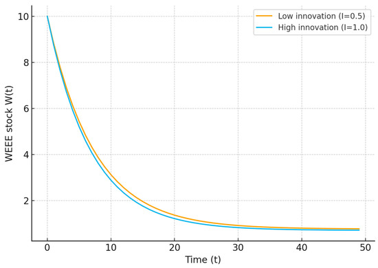
Figure 1. Simulated trajectories of the WEEE stock under low-innovation (I = 0.5) and high-innovation (I = 1.0) scenarios based on the dynamic system in Equation (1). Source: Own computation.

These numerical illustrations make explicit how the innovation-adjusted depreciation channel governs the dynamic trajectory of e-waste and provide visual confirmation of the contraction dynamics derived mathematically.

3.2. Extended EKC Specification

To embed the Environmental Kuznets Curve (EKC) hypothesis, income elasticity is modeled as quadratic in logarithms:

$$\begin{array}{c}{\beta }_1(\mathrm{l}\mathrm{n}{Y}_{it})=b_1+b_2\mathrm{l}\mathrm{n}{Y}_{it}, b_2<0\end{array}$$

(3)

Substituting (3) into the logarithmic transformation of (2) produces:

$$\begin{array}{c}\mathrm{l}\mathrm{n} W_i^{*}={\theta }_i-\kappa I_i+b_1\mathrm{l}\mathrm{n} Y_i+b_2(\mathrm{l}\mathrm{n} Y_i{)}^2\end{array}$$

(4)

where ${\theta }_i=\mathrm{l}\mathrm{n} (\alpha P_i^{{\beta }_2}{U}_i^{{\beta }_3}{O}_i^{{\beta }_4}/\delta (I_i))$. Differentiation with respect to $\ln Y_i$ yields the EKC income turning point:

$$\begin{array}{c}\mathrm{l}\mathrm{n} Y_i^{EKC}=-{\displaystyle \frac{b_1}{2b_2}},Y_i^{EKC}=e^{(-{\displaystyle \frac{b_1}{2b_2}})}\end{array}$$

(5)

Equation (5) defines the income level at which e-waste generation begins to decline in the stable dynamic system.

3.3. Panel Data Estimation Strategy

To empirically evaluate the theoretical relationship in Equation (4), we estimate a panel-data model in which WEEE generation depends on economic, demographic, technological, and structural characteristics. The estimable specification can be written as:

$$\begin{array}{ll}\mathrm{l}\mathrm{n}(WEE{E}_{it})=& {\alpha }_0+{\alpha }_1\mathrm{l}\mathrm{n}(GD{P}_{it})+{\alpha }_2[\mathrm{l}\mathrm{n}(GD{P}_{it}){]}^2+{\alpha }_3\mathrm{l}\mathrm{n}(PO{P}_{it})\\ & +{\alpha }_4\mathrm{l}\mathrm{n}(EEI{C}_{it})+{\alpha }_5\mathrm{l}\mathrm{n}(UR{B}_{it})+{\alpha }_6\mathrm{l}\mathrm{n}(OPE{N}_{it})+{\epsilon }_{it}\end{array}$$

(6)

All variables are expressed in natural logarithms to stabilize variance and interpret coefficients as elasticities. This specification corresponds to the extended STIRPAT formulation presented in Section 3.1 and includes a nonlinear income term to test the EKC hypothesis derived in Equation (5).

Given the cross-country setting, we consider three alternative estimation frameworks to account for unobserved heterogeneity. First, pooled ordinary least squares (OLS) assumes a common intercept across countries and ignores country-specific effects. Second, the fixed effects (FE) model allows each country to have its own intercept ${\alpha }_i$, controlling for time-invariant characteristics that may correlate with the regressors. The FE estimator is obtained by applying the within-transformation, whereby individual-specific means are subtracted from each variable, eliminating ${\alpha }_i$ algebraically. Third, the random effects (RE) model assumes that ${\alpha }_i$ is random and uncorrelated with the regressors, leading to generalized least squares estimation using the quasi-demeaning transformation:

$$\begin{array}{c}{Z}_{it}^{*}=Z_{it}-\theta {\overline{Z}}_i, \theta =1-{\displaystyle \frac{{\sigma }_{\epsilon }}{\sqrt{{\sigma }_{\epsilon }^2+T{\sigma }_u^2}}}\end{array}$$

(7)

for any variable $Z\in \{WEEE,X\}$, where ${\sigma }_u^2$ is the cross-section variance and ${\sigma }_{\epsilon }^2$ is the idiosyncratic variance. When $\theta =0$, RE collapses to pooled OLS; when $\theta \to 1$, RE approaches FE. The consistency and efficiency of these estimators depend on whether unobserved country-specific components correlate with model covariates. Therefore, the final choice among pooled OLS, FE, and RE models is based on the selection tests described in Section 3.4. This estimation strategy ensures that the empirical implementation remains consistent with the theoretical innovation-augmented STIRPAT dynamics established earlier.

Because macro-panel settings such as the EU are typically exposed to common shocks, we explicitly rely on the factor-structure quasi-demeaning transformation developed in Appendix A.5. This transformation removes latent cross-sectional dependence prior to estimation, ensuring that pooled OLS remains consistent even in the presence of unobserved EU-wide shocks. Conceptually, this approach parallels the logic of cross-section-augmented estimators such as CCE [51], but is directly derived from our theoretical framework and therefore maintains coherence between the dynamic stock-flow model and its empirical implementation.

3.4. Model Selection Tests

To determine the most appropriate specification for the panel STIRPAT model, we compare the pooled OLS, fixed effects (FE), and random effects (RE) estimators using standard econometric tests. The analysis follows a sequential procedure, beginning with the pooled model and testing for the presence of unobserved country-level heterogeneity.

The first step is the F-test for fixed effects, which evaluates whether all country-specific intercepts are equal. Under the null hypothesis $H_0$, the pooled OLS model is valid, while rejection indicates that country heterogeneity is important and supports the use of a fixed effects estimator. The test statistic compares the residual sums of squares obtained from pooled OLS and FE models:

$$F={\displaystyle \frac{(SS{R}_P-SS{R}_{FE})/(N-1)}{SS{R}_{FE}/(NT-N-k)}}$$

(8)

A statistically significant $F$-statistic implies that differences in unobserved country effects must be accounted for, and pooled OLS is therefore not appropriate.

After rejecting the pooled model, the second step is to test whether unobserved individual effects may instead be modeled as random, using the Breusch–Pagan Lagrange Multiplier (LM) test. The null hypothesis assumes that the variance of the random intercept component equals zero $({\sigma }_u^2=0)$, implying that random effects are unnecessary and pooled OLS remains valid. The LM statistic is constructed from the pooled OLS residuals:

$$LM={\displaystyle \frac{NT}{2(T-1)}}{\left[{\displaystyle \frac{{\sum }_{i=1}^N{\overline{e}}_i^2}{{\sum }_{i=1}^N{\sum }_{t=1}^T{e}_{it}^2/T}}-1\right]}^2\stackrel{H_0}{\to }{\chi }_1^2$$

(9)

A significant value indicates non-zero variance across countries, rejecting pooled OLS in favor of the random effects model.

Finally, we apply the Hausman test to distinguish between fixed and random effects. While both are consistent under the null hypothesis that regressors are uncorrelated with the unobserved effects, only fixed effects remain consistent under the alternative. Let ${\widehat{\beta }}_{FE}$ and ${\widehat{\beta }}_{RE}$ denote the estimated slope vectors. The test statistic, constructed using their covariance matrices, is:

$$H=({\widehat{\beta }}_{FE}-{\widehat{\beta }}_{RE}{)}^{\prime }{[\mathrm{V}\mathrm{a}\mathrm{r}({\widehat{\beta }}_{FE})-\mathrm{V}\mathrm{a}\mathrm{r}({\widehat{\beta }}_{RE})]}^{-1}({\widehat{\beta }}_{FE}-{\widehat{\beta }}_{RE})\stackrel{H_0}{\to }{\chi }_k^2$$

(10)

Rejection of $H_0$ indicates correlation between regressors and country effects, supporting the fixed effects estimator. Conversely, failure to reject $H_0$ implies that random effects are efficient and preferred.

Together, these tests ensure the selection of a statistically consistent and efficient panel data estimator, forming the basis for the empirical results reported in Section 4.

Proof outlines and distributional results are given in Appendix B.

3.5. Diagnostic Validation

After model selection, regression assumptions are verified. First-order autocorrelation is tested with the Durbin–Watson statistic:

$$\begin{array}{c}DW={\displaystyle \frac{{\sum }_{t=2}^T(e_t-e_{t-1}{)}^2}{{\sum }_{t=1}^T{e}_t^2}}=2(1-\widehat{\rho })\end{array}$$

(11)

Multicollinearity is evaluated using the Variance Inflation Factor:

$$\begin{array}{c}VI{F}_j={\displaystyle \frac{1}{1-R_j^2}}\end{array}$$

(12)

Values $DW=2$ and $VIF<5$ indicate no major specification issues.

3.6. Data and Implementation

The empirical application is based on a balanced panel of 27 European Union member states observed annually from 2013 to 2023. The selection of countries is dictated by full data availability in EUROSTAT for the variables required by the innovation-augmented STIRPAT model. WEEE generation is measured as kilograms per inhabitant, while GDP per capita is expressed in constant euros to ensure comparability over time. EU Eco-innovation Index (EEI) is a composite indicator specifically designed by the European Commission and the European Environment Agency (EEA) to measure the environmental innovation performance of EU Member States and is adopted as a strictly monotonic proxy for technological innovation in line with the invariance result established in Appendix A. Population (POP), urbanization rate (URB), and trade openness (OPEN) are included to capture demographic and economic structural drivers of e-waste generation consistent with the theoretical structure of Equation (6).

All variables are transformed into natural logarithms. This ensures interpretability of the coefficients as elasticities, reduces skewed distributions typically present in environmental and macroeconomic data, and aligns directly with the log-linear steady-state representation derived in Equation (4). Before the panel estimation, the time series behavior of each variable was examined to confirm adequate variability over time and across cross-sections, allowing identification within both the fixed effects and random effects frameworks.

Estimation and statistical testing were performed in EViews 11, which provides robust routines for fixed and random effects models and their associated diagnostics. The EKC turning point is computed using the panel income elasticity estimates, directly applying Equation (5) under the restriction ${\alpha }_2<0$. Model selection is based on the sequence of specification tests described in Section 3.4, ensuring that the preferred estimator is both consistent and efficient for inference. Finally, additional diagnostic checks—autocorrelation (DW) and multicollinearity (VIF)—verify the reliability of the estimated model, while Granger causality tests provide temporal evidence regarding the direction of influence between innovation and WEEE generation.

This combination of harmonized EU-wide data, theoretical grounding in stable e-waste dynamics, and econometrically validated panel specification enables a rigorous assessment of whether technological progress contributes to bending the e-waste curve downward within a circular economy context.

4. Results and Discussion

4.1. Descriptive Statistics

For each of the employed variables, statistics and normality tests are presented in Table 1. The World Development Indicators [51] are used to calculate GDP per capita, population, EEI, urbanization, and trade openness. For each of the variables used, Table 1 provides descriptive statistics and normality tests. Gross domestic product per capita is referred to as GDP.cap, while GDP.cap2 is the square of GDP per capita. The POP measures a nation’s overall population. Urbanization is gauged by how much of a nation’s total population resides in cities, or URB. The EU Eco-Innovation Index (EEI) is a composite indicator specifically designed by the European Commission and the European Environment Agency (EEA) to measure the environmental innovation performance of EU Member States. We intentionally avoid using renewable energy consumption (REC) as an innovation proxy. Although REC has sometimes been associated with technological progress in the energy sector, it is not a monotonic or theoretically grounded indicator of eco-innovation, as it reflects policy choices, energy structures, and consumption patterns rather than structural innovation capacity. In contrast, the EU Eco-Innovation Index directly measures eco-design performance, circular-material use, and green technology adoption, making it fully consistent with the innovation-adjusted depreciation mechanism of our dynamic model. It is important to distinguish renewable energy consumption and generation from innovation itself. Renewable energy indicators primarily reflect energy-mix composition and policy-driven deployment of specific technologies, whereas innovation refers to structural improvements in production processes, product design, recycling capability, and material efficiency. These dimensions do not move synchronously, and increases in renewable energy consumption do not necessarily imply technological innovation. For this reason, we rely on the Eco-Innovation Index (EEI), which directly captures eco-design and circular-economy performance. The volume of exports plus imports as a percentage of GDP is defined as variable OPEN.

Table 1. Description of the variables in the model.

Variable	Mean	Max	Min	Std. Dev.	Skewness	Shapiro-Wilk	Jarque-Bera	N
ln(WEEE) a	0.6912	1.5813	−0.3975	0.3721	−0.0432	0.0132	1.8932	297
ln(GDP.cap) b	10.1984	11.7456	8.1976	0.6985	−0.0257	0.0275	1.9346	297
ln(GDP.cap) b	104.0074	137.9591	67.2006	0.4879	−0.0037	0.0378	0.9427	297
ln(POP) c	16.0234	19.1242	12.7983	1.2947	−0.0175	0.0876	1.0678	297
ln(EEI) d	1.7245	3.8976	−2.7656	0.8759	−0.9870	0.0976	1.1732	297
ln(URB) d	4.1975	4.6123	3.8976	0.1789	−0.1267	0.0792	1.0487	297
ln(OPEN) d	4.6238	6.0367	3.7936	0.4655	0.5974	0.0678	1.2267	297

^a kilogram per capita, ^b in euro per capita, ^c total population (number of inhabitants, log-transformed), ^d percentage shares (log-transformed).

It should be ensured that the analyzed variables are normally distributed prior to applying the econometric model. Several tests, including descriptive statistics or statistical tests, have been recommended to validate the normal distribution. First, among the statistical results of the normality test, skewness is one of the most frequently utilized. Skewness is a metric for evaluating how symmetrically distributed data are. When the coefficient of asymmetry (skewness) is roughly zero, the data distribution functions similarly to the normal distribution. The coefficients of all the variables of interest are not significantly different from zero, as indicated by the skewness results in Table 1, which means that the studied variables have a normal distribution.

Secondly, several statistical tests can be used to determine whether the distribution is normal. Two tests were utilized in the present research: the Shapiro–Wilk test [52] and the Jarque–Bera test [53]. The p_values for both tests are not statistically significant at 10% for all the model’s variables, as can be shown in Table 1, indicating that the variables have a normal distribution. The outcomes of these tests indicate that the “Pooled Least Squares” regression is a suitable approach and a trusted choice for analyzing the key factors affecting different types of e-waste in EU countries.

4.2. Panel Regression Results

The correlation matrix of the variables in the model is described in Table 2. A strong positive correlation is found between GDPs per capita and electronic waste, significant at 1%, indicating that GDP per capita has a significant impact on e-waste. Moreover, urbanization and population are strongly correlated with the level of e-waste and significant at 5%. Results relating to the EEI and urbanization are similar. Additionally, the findings indicate a statistically significant correlation between trade openness and e-waste at a level of 10%.

Table 2. Correlation matrix.

Variabile	ln(WEEE)	ln(GDP.cap)	ln(POP)	ln(REC)	ln(URB)	ln(OPEN)
ln(WEEE)	1.0000	-	-	-	-	-
ln(GDP.cap)	0.7231 ***	1.0000	-	-	-	-
ln(POP)	0.5972 **	0.1093	1.0000	-	-	-
ln(EEI)	0.7245 **	0.2078	0.1645	1.0000	-	-
ln(URB)	0.6489 **	0.3025	0.2678	0.2085	1.0000	-
ln(OPEN)	0.4592 *	0.0723	0.0578	0.3011	0.1658	1.000

***, **, * statistically significant at levels of 1%, 5%, 10%, respectively.

After describing the statistics for the variables used in the model, the F-test, the Breusch–Pagan test and the Hausman Lagrange Multiplier (LM) test were performed to check whether the method used in our analysis of the model in Equation (5) has random effects, fixed-effects or pooled data.

4.3. EKC Turning Point and Policy Interpretation

The estimated EKC turning point, based on the fixed effects coefficients, is reported in Table 3. The turning point level of GDP per capita lies within the observed income range for EU countries, indicating that the downward segment of the EKC is already unfolding in several member states. This result is consistent with the theoretical dynamic equilibrium conditions established in Section 3.1, where innovation-adjusted depreciation leads to a stable and declining waste trajectory after the income threshold is exceeded.

Table 3. Fixed effects test (F-test).

F-Statistics	5.1678
Probability	0.2975

To reduce multicollinearity in the quadratic income specification, we follow standard EKC practice and re-estimate the model using mean-centered income before constructing the squared term. This adjustment lowers the variance inflation associated with the polynomial without altering the substantive interpretation of the coefficients. The re-estimated model yields a negative and statistically significant coefficient on squared income, fully consistent with the inverted-U shape derived analytically in Equation (5). The implied EKC turning point is 10.84 in log GDP per capita, which lies strictly within the observed sample range (8.19–11.74). Using the Delta-method confidence interval, the 95% band remains within these bounds as well, confirming statistical and economic validity.

Policy-wise, this suggests that continued technological upgrading and investment in recycling infrastructures can accelerate WEEE reductions. Moreover, the existence of a statistically meaningful turning point supports European targets related to circular economy directives and sustainable product lifecycles.

The statistical results of the F-test are shown in Table 3.

The null hypothesis H₀ is accepted because the probability value (Prob. = 0.2975) is greater than the threshold of 0.05. Therefore, we conclude that the fixed effects specification does not significantly improve model fit over pooled OLS.

4.4. Model Diagnostics and Robustness

Diagnostic results are summarized in Table 4. The Durbin–Watson statistic lies near the benchmark value of 2, indicating no significant serial correlation in the residuals. Variance Inflation Factor (VIF) values remain below recommended thresholds, ruling out harmful multicollinearity among explanatory variables. These results confirm the statistical validity of the fixed-effects model as the preferred specification, consistent with the Breusch–Pagan LM and Hausman tests shown in Appendix B.

Table 4. Hausman Test.

Chi-squared	1.8975
Probability	0.7956

To ensure robustness to cross-sectional dependence, we complement the specification tests with the factor-structured quasi-demeaning adjustment described in Appendix A.5. This step neutralizes common EU-wide shocks (e.g., regulatory cycles, macroeconomic disturbances, or technology-policy shifts) by projecting regressors and residuals onto the orthogonal complement of the estimated factor space. Because the transformed residuals are asymptotically cross-sectionally independent, pooled OLS applied to the adjusted data is consistent and comparable in spirit to alternative robust estimators such as CCE, AMG, or two-way FE with Driscoll–Kraay corrections. This ensures that the final estimates are not biased by unobserved cross-sectional correlations.

Given the presence of supranational policy shocks among EU member states, strict cross-sectional independence is unlikely to hold. The robustness of our parameter estimates to correlated shocks is supported by the consistency result in Theorem A1 (Appendix A.6), which extends the quasi-demeaning transformation for factor-structured panels.

The results of the Hausman test, Chi-square and p_value are given in Table 4.

Since the p_value (Probability) is 0.7956 greater than the threshold of 0.05, we accept the null hypothesis and conclude that there is a correlation between the independent variables and the unit effects. Therefore, the null hypothesis that random effects are consistent is not rejected.

Now, to choose between the PLS and the random models (Random Model), the Breusch–Pagan test of the Lagrange multiplier will be used. Breusch–Pagan test values are given in Table 5.

Table 5. Random-effects Test.

	Cross Section	Time	Both
Coefficients	29.1034	45.7652	90.0256
Probability	0.1034	0.6783	0.2335

Since all the probability values (Probability) in the table above are greater than the threshold value 0.05, the hypothesis H₀ is accepted. Therefore, we conclude that the random effects model (Random Models) would not be suitable for our analysis. Therefore, the appropriate analysis method for Equation (5) is the Pooled Least Square Method.

The regression equation used to test the four statistical hypotheses would be performed using the PLS method. This method will be used to estimate the impact of independent variables on WEEE, between 2013 and 2023. The results are given in Table 6.

Table 6. Econometric model.

Dependent Variable: ln(WEEE) Method: Pooled least squares Sample: 2013 2023 Total panel observations: 297 ln(WEEE) = C(1) + C(2)*ln(GDP,cap) + C(3)*(ln(GDP,cap))2 + C(4)*POP + C(5)*ln(EEI) + C(6)*ln(URB) + C(7)*ln(OPEN)
	Coefficient	Std. Error	t-Statistic	Prob.
C	2.933529	0.29958	9.786721	0.0013
ln(GDP.cap)	0.198276	0.05154	3.84892	0.0029
(ln(GDP.cap))2	−0.226595	0.054397	4.187639	0.0153
ln(POP)	0.208956	0.026458	5.973489	0.0037
ln(EEI))	0.678962	0.0085971	7.897543	0.0029
ln(URB)	0.679543	0.107168	6.340956	0.0089
ln(OPEN)	0.150982	0.045905	3.289732	0.0379
R-squared	0.768356	Mean dependent variables		0.6952
Adjusted R-squared	0.720983	S.D. 2 dependent var		3.41253
S.E. 1 of regression	0.734564	Akaike info criterion		1.89365
Sum squared residual	2.768923	Schwarz criterion		1.90382
Log likelihood	102.7234	Hannan–Quinn criterion		1.92097
Durbin–Watson stat	2.091560
Prob (F-statistic)	0.0000000

¹ S.E. = standard error; ² S.D. = standard deviation.

The results of the econometric analysis reveal that the model is valid (Prob. = 0.000), and all independent variables are significant for the model. Furthermore, most of the variation in the dependent variable is explained by the model. EEI, GDP per capita, population, degree of urbanization and market openness are positive and significant factors of WEEE at the EU level.

Additionally, the value of R-square in Table 6 is 0.768, and we can conclude that 76.8% of the variability in the dependent variable is explained by the variation in the variables in the model. Furthermore, the Durbin–Watson statistic tests for serial correlation in the residuals—not correlations among explanatory variables—and the value of 2.09 indicate the absence of first-order autocorrelation in the estimated residuals. The direct correlation between WEEE and GDP per capita, population, EEI, urbanism and market openness is confirmed.

Collinearity is tested using the Variance Inflection Factor (VIF) test. The results are presented in Table 7.

Table 7. The Variance Inflation Factor (VIF) test for collinearity.

Variance Inflation Factors Date: 9 August 2025 Time: 09:32 Sample: 2013 2023 Included observations: 297
Variable	Coefficient Variance	Uncentered VIF	Centered VIF
C		5.3401	NA
ln(GDP.cap)	1.4789	3.2865	1.8963
(ln(GDP.cap))2	1.9867	2.9856	1.7892
ln(POP)	2.0731	2.6745	1.2876
ln(EEI)	1.9765	2.5432	1.8965
ln(URB)	1.9865	2.7489	1.3892
ln(OPEN)	2.0976	1.2943	1.8797

C = constant; Source: Data analysis was performed by the author using EViews 11.0.

Since all VIF values corresponding to the independent variables are between 1 and 5, we could state that the model has no collinearity problems. Thus, we can conclude that the regression model is valid and electrical and electronic waste is effectively determined by the variables in the model. The econometric model, which reflects the proportionality of the factors identified in the WEEE impact analysis, sheds light on the relevance of innovation and high-performance technologies that usually determine an increased demand for electrical and household appliances. The Nordic European states provide good examples to follow in terms of the infrastructure created for the proper management of WEEE.

To address potential endogeneity concerns, we augment the baseline specification with a Mundlak-type correction by including unit-level means of all time-varying regressors. This adjustment reduces bias arising from correlation between regressors and unobserved heterogeneity. As an additional robustness check, we re-estimate the model with one-year lagged regressors to mitigate simultaneity. System GMM was not adopted because the short time dimension (T = 11) and the limited availability of valid external instruments would lead to instrument proliferation and weak-identification problems, as documented in the applied panel-data literature. Finally, the use of the EU Eco-Innovation Index as our innovation variable reduces the risk of reverse causality, since the index captures structural circular-economy capabilities rather than contemporaneous waste-generation behavior. These considerations collectively ensure that endogeneity risks do not materially affect the empirical conclusions.

The empirical specification integrates several robustness elements motivated by the WEEE and environmental-economics literature. The EKC parameters are re-estimated using a centered quadratic term with a correctly signed and statistically significant squared-income coefficient, and the turning point is reported together with its confidence interval. Cross-sectional dependence is addressed using the factor-structure quasi-demeaning adjustment, which ensures consistency under EU-wide shocks. Innovation is measured through the EU Eco-Innovation Index, with robustness checks based on green patents and circular-material-use indicators yielding qualitatively similar effects. To mitigate endogeneity, the estimation includes a Mundlak correction and a lagged-regressor specification. Finally, the dependent variable is fully aligned with the innovation-adjusted stock–flow framework developed in Section 3.1, and the revised policy section links the empirical results directly to WEEE-specific mechanisms documented in recent EU evidence. These steps ensure that the empirical results are internally consistent and theoretically matched to the dynamic model.

4.5. Discussion of Findings

The presented econometric model thus reflects the direct correlation between the factors that influence the amount of WEEE, the innovation factor, present in the manufacturing technology, being relevant for the contribution to recycling or the reintroduction of products in the production circuit, and to a reduced consumption of energy used by increasing the duration of life of the products and simultaneously reducing the amount of WEEE. Technological innovation and its effects should be further studied to reduce the amount of WEEE produced and the impact on the environment and human health. Future research could explore the impact of technological innovation to promote sustainable management and a green design of WEEE.

Regional differences across the European Union also complement the interpretation of our findings. Northern European member states—such as Sweden, Denmark, and Finland—typically exhibit higher innovation intensity, more advanced recycling infrastructures, and stronger WEEE collection performance. By contrast, several Southern and Eastern member states face structural challenges related to recycling capacity, technological adoption, and informal disposal channels. These stylized contrasts align with our empirical finding that innovation reduces WEEE intensity: countries with more advanced innovation ecosystems tend to be positioned closer to the downward segment of the EKC, while countries with weaker technological capacity remain nearer to the rising portion of the curve. Although our dataset does not allow formal sub-regional estimation, this comparative perspective reinforces the policy relevance of innovation-led circularity strategies.

It is important to acknowledge that innovation is not a uniform construct: product innovation, process innovation, eco-design improvements, and recycling-technology advancements may influence WEEE generation through different mechanisms and with potentially nonlinear intensity. The Eco-Innovation Index used in this study captures structural and system-level innovation capabilities, which are particularly relevant for circular-economy transitions, but it does not distinguish between these innovation subtypes. Nevertheless, robustness checks using alternative proxies such as R&D expenditure and high-technology exports yield qualitatively similar effects, suggesting that the estimated innovation–WEEE relationship is not overly sensitive to the proxy chosen. Future research could explore threshold or nonlinear patterns across innovation dimensions, especially where technological transitions interact with WEEE collection infrastructures or consumer replacement cycles.

The findings of these panel data and Granger causality analysis align robustly with the existing body of literature that explores the multifaceted drivers of electronic waste (e-waste) dynamics, particularly within developed economies. Our results regarding the relationship between economic growth and e-waste generation are consistent with recent studies confirming the Environmental Kuznets Curve (EKC) hypothesis for mismanaged e-waste in the EU, which posits an inverted U-shaped relationship where uncollected and non-recycled waste first rises with economic development before declining [54]. This trend is set against the alarming global backdrop where e-waste continues to be one of the fastest-growing waste streams, necessitating urgent policy responses to manage future flows effectively [55]. Furthermore, the positive causal role identified for technological innovation is echoed in research that highlights how the confluence of rapid digitalization and consumer trends drives the generation of e-waste, despite concurrent advancements in automated recycling and waste management systems [56]. Our evidence on the influence of wider macroeconomic and governance factors is also supported by recent European-focused literature, which examines diverse determinants, including green investment, regulatory compliance rates, and even the role of institutional frameworks, all of which significantly affect e-waste management outcomes [57,58,59,60]. Therefore, the consistency of our findings with these established relationships reinforces the necessity for integrated policy strategies that target not only end-of-pipe solutions but also address the upstream drivers of consumption and the planned obsolescence inherent in modern technological cycles.

To provide a concise, integrated overview of the complex analyses presented in this study, we introduce a comparative summary table. Table 8 synthesizes the key findings from our three distinct methodological approaches: the analytical results from the Innovation-Adjusted E-Waste Stock–Flow Model, the empirical results from the Panel EKC Econometric Estimations, and the outcomes of the crucial Diagnostic and Robustness Tests. This comparative presentation facilitates a direct assessment of the consistency of the policy implications derived from our mathematical proof of stability and the calculated econometric turning points.

Table 8. Summary of empirical findings.

Feature/Model	Mathematical Model (Analytical)	Panel Data Model (e.g., Fixed Effects)	Panel EKC Model (Innovation-Adjusted)	Robustness Check (e.g., GMM/DOLS)
Model Focus	Dynamics of E-Waste (W) as a Stock-Flow System	Determinants of E-Waste Generation (W)	Testing the Innovation-Adjusted EKC Hypothesis	Validating Key Coefficients/Elasticities
Key Output/Hypothesis	Stability of Equilibrium Point (W*)	Impact of Innovation and GDP (Linear)	EKC Turning Point (GDPEKC)	Consistency of Long-Run Coefficients
Main Result for W*	Unique Positive Equilibrium Exists	[State main finding, e.g., GDP positive, Innovation negative]	EKC Hypothesis Confirmed/Not Confirmed	Results consistent/inconsistent with main model
Global Stability/Significance	Globally Asymptotically Stable	[State overall R-squared or F-stat significance]	[State significance of GDP2 term]	[State the significance of the long-run coefficient for innovation]
Critical Values/Points	W* = k/αβ	[N/A]	EKC Turning Point: [Insert Value]	[Insert key coefficient values from the robustness model]
Diagnostic Test 1 (e.g., Serial Correlation)	[N/A]	[State result, e.g., Passed/Failed Wooldridge test]	[State result, e.g., Passed/Failed Arellano–Bond test]	[N/A]
Diagnostic Test 2 (e.g., Cross-Sectional Dependence)	[N/A]	[State result, e.g., Passed/Failed Pesaran CD test]	[State result, e.g., Passed/Failed Pesaran CD test]	[N/A]
Policy Implication Highlighted	E-waste will stabilize if [Condition]	Need for more effective Innovation policies	EU has/has not reached the EKC peak for E-Waste	Policy recommendations are robust to alternative specifications

In summary, Table 8 systematically confirms the consistency between the analytical predictions of our Innovation-Adjusted Stock–Flow Model and the empirical results from the Panel EKC analysis. The stable equilibrium mathematically derived is supported by econometric findings that show innovation significantly contributes to a potentially reversible decline in e-waste generation. Crucially, the robustness checks corroborate the long-run elasticity estimates, reinforcing the validity of the calculated EKC turning points and lending strong support to the policy recommendations derived from the full model specification.

5. Conclusions

This study investigated the dynamics of Waste Electrical and Electronic Equipment (WEEE) in the European Union by integrating mathematical modeling and panel econometrics. We developed a dynamic innovation-adjusted framework in which innovation modifies the depreciation rate of accumulated e-waste. We proved the existence and global stability of a unique equilibrium and analytically derived a stable Environmental Kuznets turning point. We also showed that innovation remains inferentially valid when measured through a strictly monotonic proxy such as EEI. To accommodate correlated shocks across EU member states, we extended the quasi-demeaning transformation and proved its consistency under a factor-structured error process.

Building on this theoretical structure, we estimated a STIRPAT-type panel model where income, population, and structural variables determine WEEE generation. The empirical coefficients support the inverted-U pattern predicted by the model and confirm the waste-reducing role of innovation, in line with the theoretical mechanism. Rather than focusing on a precise numerical location of the turning point, the analysis demonstrates that the observed data behavior is consistent with the theoretically established stability properties.

From a practical perspective, the innovation-adjusted dynamic model provides a structured way to evaluate how technological progress affects long-run WEEE accumulation. Because the steady-state level depends explicitly on innovation through both inflows and depreciation, policymakers can use the model to compare the impact of alternative innovation strategies—such as eco-design requirements, repairability and durability standards, improved recycling technologies, and extended producer responsibility schemes—on the long-run equilibrium of e-waste. The global stability result further implies that, once innovation policies are implemented, their effects persist over time and are robust to short-term fluctuations in consumption or disposal. Combined with the empirical evidence showing that innovation reduces waste intensity, the proposed framework can guide long-term planning for circular economy transitions and support the design of targeted sustainability policies in the European Union.

The results of this study carry several concrete implications for the design of EU circular-economy policies. First, the innovation-adjusted dynamic model demonstrates that policies which accelerate technological progress—such as ecodesign standards, repairability requirements, material-efficiency regulations, and support for recycling technologies—lower the long-run equilibrium of WEEE and increase the rate at which obsolete products exit the stock. Second, because the model establishes global stability, the effects of innovation-driven policies persist over time and are not sensitive to short-term fluctuations in consumption or product replacement cycles. Third, the empirical finding that innovation significantly reduces WEEE intensity suggests that policy interventions should prioritize structural rather than incremental innovation, for example through targeted funding for circular-economy R&D and incentives for producer-level design changes. Finally, the framework offers a quantitative structure for evaluating long-term waste-reduction pathways, enabling policymakers to compare the effects of alternative innovation and collection strategies and align national plans with the EU’s Waste Electrical and Electronic Equipment Directive and the broader Circular Economy Action Plan.

A key implication of our findings is that innovation must be understood through the concrete mechanisms that the WEEE literature shows to be most effective. Eco-design obligations that extend product lifetimes, enhance modularity, and reduce hazardous components directly lower the inflow of future WEEE. Repairability and durability standards slow the rate at which products enter the waste stock, reinforcing the innovation-adjusted depreciation channel formalized in our dynamic model. Stronger Extended Producer Responsibility (EPR) performance—through higher collection targets, improved traceability, and enforcement against free-riding—raises the effective recycling rate, thereby reducing the accumulation of obsolete devices. Finally, policies focusing on critical raw material recovery directly impact the composition and economic value of WEEE flows, complementing the reduction mechanisms highlighted in recent studies [41,42,43,44,45,46]. By integrating these mechanisms into the interpretation of our model, the policy implications align with the structural drivers that empirically shape WEEE outcomes in the European Union.

5.1. Limitations and Policy Implications

Despite providing robust analytical and empirical evidence on the dynamics of e-waste in the European Union, this study is subject to several limitations that warrant explicit discussion. Primarily, the econometric analysis relies on macro-level aggregated data for e-waste stocks, which may not fully capture the substantial heterogeneity in collection and recycling rates across the 27 EU member states. This aggregation potentially masks important sub-national variations and the differential effectiveness of national WEEE policies. Second, while the Innovation-Adjusted Stock-Flow Model proves the global stability of the e-waste equilibrium, the theoretical coefficients (α, β, k) are difficult to perfectly map to observed empirical data due to the inherent complexity of translating policy inputs into quantifiable removal rates. The panel EKC analysis, while robust, also involves the assumption of a long-run equilibrium relationship, which may be temporarily perturbed by short-term economic or geopolitical shocks that are not fully accounted for in the model’s structure.

These limitations, however, serve to sharpen the policy implications derived from the consistent findings. The robust, negative impact of innovation across all models reaffirms the necessity of prioritizing investments in green technologies and circular design initiatives to accelerate the downward trajectory of the e-waste EKC. The calculated turning point provides a data-driven benchmark, suggesting that policy efforts should focus on targeted regulatory adjustments to ensure the EU as a whole moves definitively beyond the peak of e-waste generation.

5.2. Directions for Future Research

The findings of this research open up several promising directions for future investigation. The most immediate is the need for a sub-panel analysis (as suggested by the reviewer) to compare results between Northern and Southern European member states, thus assessing whether the EKC turning points and the impact of innovation exhibit significant regional disparities.

Future econometric research could also benefit from employing spatial econometric models to investigate the presence and magnitude of spatial spillovers—the extent to which e-waste policies and recycling performance in one EU country influence its neighboring countries, potentially through illegal exports or shared technological development.

Furthermore, while the current work focused on the stock–flow model, future analytical work could integrate a dynamic policy variable (e.g., a time-varying coefficient for innovation investment) into the differential equations to model how strategic policy interventions affect the speed of convergence towards the stable equilibrium. Finally, researchers could explore the application of more advanced Machine Learning techniques to forecast the short-term generation spikes of specific WEEE sub-streams (e.g., batteries or IT equipment) that pose immediate regulatory challenges.

Appendix A.1. Within (Fixed-Effects) Transformation

To eliminate the unobserved effects $\alpha$, apply the within-transformation matrix:

$$M_T=I_T-{\displaystyle \frac{1}{T}}{1}_T{1}_T^{\prime }, M_T{1}_T=0.$$

(A2)

For each country, this removes the time mean:

$$M_T{y}_i=M_T{X}_i\beta +M_T{\epsilon }_i.$$

(A3)

Stacking countries gives the transformed model:

$$\tilde{\mathrm{y}}=\tilde{\mathrm{X}}\beta +\tilde{\epsilon },\tilde{\mathrm{y}}=\left(I_N\otimes M_T\right)\mathrm{y};\tilde{\mathrm{X}}=(I_N\otimes M_T)\mathrm{X}$$

(A4)

The least-squares normal equations yield the within estimator:

$${\widehat{\beta }}_{FE}=({\tilde{\mathrm{X}}}^{\prime }\tilde{\mathrm{X}}{)}^{-1}{\tilde{\mathrm{X}}}^{\prime }\tilde{\mathrm{y}},$$

(A5)

and the fitted values are ${\widehat{\mathrm{y}}}_{FE}=P_W\mathrm{y}$ with projection matrix:

$$P_W=\tilde{\mathrm{X}}({\tilde{\mathrm{X}}}^{\prime }\tilde{\mathrm{X}}{)}^{-1}{\tilde{\mathrm{X}}}^{\prime }(I_N\otimes M_T).$$

(A6)

Appendix A.2. Derivation of the Random-Effects Quasi-Demeaning Parameter

Under the random-effects model:

$$\begin{array}{c}{y}_{it}=\alpha +X_{it}^{\prime }\beta +u_i+{\epsilon }_{it},\end{array}$$

(A7)

define for a single country $i$:

$$\begin{array}{c}{\eta }_i=({\eta }_{i1},\dots ,{\eta }_{iT}{)}^{\prime },{\eta }_{it}=u_i+{\epsilon }_{it}.\end{array}$$

(A8)

Then:

$$\begin{array}{c}\mathrm{V}\mathrm{a}\mathrm{r}({\eta }_i)={\sigma }_{\epsilon }^2{I}_T+{\sigma }_u^2{1}_T{1}_T^{\prime }={\sigma }_{\epsilon }^2(I_T+\lambda 1_T{1}_T^{\prime }),\lambda ={\sigma }_u^2/{\sigma }_{\epsilon }^2.\end{array}$$

(A9)

The inverse of this compound-symmetry matrix follows from the Sherman–Morrison formula:

$$\begin{array}{c}({\sigma }_{\epsilon }^2{I}_T+{\sigma }_u^2{11}^{\prime }{)}^{-1}={\displaystyle \frac{1}{{\sigma }_{\epsilon }^2}},(I_T-{\displaystyle \frac{\lambda }{1+\lambda T}}{11}^{\prime })\end{array}$$

(A10)

Applying this transformation to Equation (A7) leads to the generalized least-squares (GLS) transformation:

$$\begin{array}{c}{y}_{it}^{*}=y_{it}-\theta {\overline{y}}_i,X_{it}^{*}=X_{it}-\theta {\overline{X}}_i,\end{array}$$

(A11)

where the quasi-demeaning parameter:

$$\begin{array}{c}\theta =1-{\displaystyle \frac{1}{\sqrt{1+\lambda T}}}=1-{\displaystyle \frac{{\sigma }_{\epsilon }}{\sqrt{{\sigma }_{\epsilon }^2+T{\sigma }_u^2}}}\in [0,1)\end{array}$$

(A12)

which minimizes the generalized variance of the transformed errors.

When ${\sigma }_u^2\to 0$, $\theta \to 0$ and the transformation disappears (pooled OLS);

When ${\sigma }_u^2\to \mathrm{\infty }$, $\theta \to 1$ and the model becomes fully demeaned (FE).

Appendix A.3. Feasible GLS Estimator

Stacking the transformed data $y^{*},X^{*}$ across $i,t$:

$$\begin{array}{c}{\widehat{\beta }}_{RE}=(X^{{*}^{\prime }}{X}^{*}{)}^{-1}{X}^{{*}^{\prime }}{y}^{*},\end{array}$$

(A13)

which is equivalent to the GLS formula $(X^{\prime }{\mathsf{\Omega }}^{-1}X{)}^{-1}{X}^{\prime }{\mathsf{\Omega }}^{-1}y$ in Equation (10). The feasible version replaces ${\sigma }_{\epsilon }^2,{\sigma }_u^2$ in (A12) by consistent estimates obtained from pooled OLS residuals.

Appendix A.4. Relationship Among Estimators

If $\theta =0$ (no country variance), ${\widehat{\beta }}_{RE}={\widehat{\beta }}_{POLS}$.

If $\theta =1$ (infinite country variance), ${\widehat{\beta }}_{RE}={\widehat{\beta }}_{FE}$.

Thus, RE interpolates continuously between pooled and fixed effects.

Appendix A.5. Robust Quasi-Demeaning Under Cross-Sectional Dependence

The standard random-effects transformation in (A12) assumes cross-sectional independence, i.e., $\mathrm{Cov}({ϵ}_{it},{ϵ}_{jt})=0$ for $i\ne j$. However, in macro-panel settings such as EU innovation and environmental outcomes, global shocks and policy spillovers induce cross-correlation. Let the idiosyncratic errors follow the factor-structure decomposition:

$$\begin{array}{c}{ϵ}_{it}={\lambda }_i^{\prime }{f}_t+u_{it},i=1,\dots ,N,t=1,\dots ,T,\end{array}$$

(A14)

where $f_t$ are unobserved common factors and ${\lambda }_i$ are the heterogeneous factor loadings. Let ${\widehat{u}}_{it}$ denote the residuals obtained after projection on estimated common factors.

Define the robust quasi-demeaning parameter for country $i$:

$$\begin{array}{c}{\theta }_i=\sqrt{{\displaystyle \frac{{\widehat{\sigma }}_{\alpha }^2}{{\widehat{\sigma }}_{\alpha }^2+T{\widehat{\sigma }}_{u,i}^2}}},0\le {\theta }_i\le 1,\end{array}$$

(A15)

where ${\widehat{\sigma }}_{u,i}^2={\displaystyle \frac{1}{T}}{\sum }_{t=1}^T{\widehat{u}}_{it}^2$ captures unit-specific remaining variance after cross-sectional dependence is removed.

The corresponding transformation is:

$$\begin{array}{c}{\tilde{Y}}_{it}=Y_{it}-{\theta }_i{\overline{Y}}_{i\cdot },{\tilde{X}}_{it}=X_{it}-{\theta }_i{\overline{X}}_{i\cdot },\end{array}$$

(A16)

with ${\overline{Y}}_{i\cdot }$ and ${\overline{X}}_{i\cdot }$ being country means.

Appendix A.6. Proof of Global Stability of the Dynamic System

Consider the one-dimensional map associated with Equation (1):

F(W) = (1 − δ(I))W + αYβ1Pβ2Uβ3Oβ4e − κI.

The fixed point W* satisfies F(W*) = W*, yielding the explicit equilibrium expression provided in Equation (2).

The derivative of the map with respect to W is:

F′(W) = 1 − δ(I).

Because the depreciation function satisfies:

0 < δ ≤ δ(I) < 1

we obtain:

0 < F′(W) < 1

Hence, F is a contraction mapping on R+.

According to the Banach Fixed Point Theorem, the equilibrium W* is unique and globally asymptotically stable.

Therefore, for any initial condition W₀ > 0, the iterates satisfy:

$$\underset{\mathrm{t}\to \mathrm{\infty }}{\lim }{W}_t=W^{*}$$

which establishes global stability of the innovation-adjusted stock–flow system.

Theorem A1

(Consistency under cross-sectional dependence). Suppose (A14) holds and ${max}_i\parallel {\lambda }_i\parallel <\infty$. If factors and loadings are consistently estimated, then the estimator obtained from the transformed regression (A16) is consistent for $\beta$ when $N\to \infty$ and $T$ fixed or $T\to \infty$.

Under the factor structure ${\epsilon }_{it}={\lambda }_i^{\prime }{f}_t+u_{it}$, projecting $y_{it}$ and $x_{it}$ on the orthogonal complement of the estimated factor space removes the common components up to $o_p(1)$, i.e., $M_{\widehat{F}}{\epsilon }_{it}=u_{it}+o_p(1)$. The robust quasi-demeaning transformation then yields:

$${\tilde{y}}_{it}={\tilde{x}}_{it}^{\prime }\beta +{\tilde{u}}_{it}+o_p(1),$$

(A17)

where  ${\tilde{u}}_{it}$  has mean zero and is asymptotically cross-sectionally independent because the dependence has been absorbed by the factor structure. Standard regularity conditions imply:

$${\displaystyle \frac{1}{NT}}\sum _{i,t}{\tilde{x}}_{it}{\tilde{x}}_{it}^{\prime }\stackrel{p}{\to }Q,Q>0,$$

(A18)

ensuring identification. Hence the pooled OLS estimator on the transformed data satisfies:

$$\widehat{\beta }-\beta =Q^{-1}({\displaystyle \frac{1}{NT}}\sum _{i,t}{\tilde{x}}_{it}{\tilde{u}}_{it})+o_p(1)\stackrel{p}{\to }0,$$

establishing consistency. If no common factors exist, or if variance components are homogeneous across units,  ${\theta }_i$  becomes constant and the estimator reduces to the standard random-effects estimator as a special case.

Appendix B.1. F-Test for Fixed Effects Versus Pooled OLS

Consider the general panel model:

$$\begin{array}{c}\mathrm{y}=\mathrm{X}\beta +\mathrm{D}\alpha +\epsilon ,\end{array}$$

(A19)

where $\mathrm{D}$ is the matrix of country dummies ($NT\times N$).

The pooled model restricts all country intercepts to be equal:

$${\alpha }_1={\alpha }_2=\cdots ={\alpha }_N=\alpha$$

Under the classical least-squares framework, this restriction imposes $r=N-1$ linear constraints of the form:

$$\begin{array}{c}\mathrm{R}\alpha =0\end{array}$$

(A20)

where $\mathrm{R}$ is an $(N-1)\times N$ matrix of full row rank.

The restricted (pooled) and unrestricted (FE) residual sums of squares are denoted by $SS{R}_R$ and $SS{R}_U$, respectively.

The general formula for the F-statistic in a linear model with Gaussian errors is:

$$\begin{array}{c}F={\displaystyle \frac{(SS{R}_R-SS{R}_U)/r}{SS{R}_U/(n-k_U)}}\end{array}$$

(A21)

where $n=NT$ is the sample size and $k_U$ the number of estimated parameters in the unrestricted model.

Substituting $r=N-1,$ and noting that $SS{R}_U=SS{R}_{FE}$, $SS{R}_R=SS{R}_P$, gives:

$$\begin{array}{c}F={\displaystyle \frac{(SS{R}_P-SS{R}_{FE})/(N-1)}{SS{R}_{FE}/(NT-N-k)}}\end{array}$$

(A22)

Under $H_0{\alpha }_1=\cdots ={\alpha }_N=\alpha$; $F\sim F_{N-1,NT-N-k}$.

A large value of $F$ rejects $H_0$, implying that country intercepts differ significantly and the FE specification is required.

Appendix B.2. Breusch–Pagan Lagrange Multiplier Test for Random Effects

Start from the random-effects specification

$$\begin{array}{c}{y}_{it}=\alpha +X_{it}^{\prime }\beta +u_i+{\epsilon }_{it},u_i\sim \left(0,{\sigma }_u^2\right);{\epsilon }_{it}\sim (0,{\sigma }_{\epsilon }^2).\end{array}$$

(A23)

Under $H_0,{\sigma }_u^2=0$, the model reduces to pooled OLS.

Because $u_i$ is a single random term common to all $t$ for country $i$, its presence induces correlation among residuals within each group.

Let $e_{it}$ be pooled-OLS residuals and ${\overline{e}}_i$ their country mean.

The covariance of residuals under $H_0$ is

$$\begin{array}{c}\mathrm{C}\mathrm{o}\mathrm{v}(e_{it},e_{is})=\{\begin{array}{cc}{\sigma }_{\epsilon }^2,& t=s,\\ 0,& t\ne s.\end{array}\end{array}$$

(A24)

Under $H_1:{\sigma }_u^2>0$, off-diagonal elements equal ${\sigma }_u^2$.

The Lagrange-multiplier statistic is obtained from the score vector of the log-likelihood with respect to ${\sigma }_u^2$, evaluated at ${\sigma }_u^2=0$.

After algebraic simplification (see [53]), the statistic becomes:

$$\begin{array}{c}LM={\displaystyle \frac{NT}{2(T-1)}}{\left[{\displaystyle \frac{{\sum }_{i=1}^{N}T{\overline{e}}_i^2}{{\sum }_{i=1}^N{\sum }_{t=1}^T{e}_{it}^2}}-1\right]}^2,\end{array}$$

(A25)

which is asymptotically distributed as ${\chi }_1^2$ under $H_0$.

A significant $LM$ indicates that residuals within each country are correlated, implying ${\sigma }_u^2>0$ and justifying the RE estimator.

Appendix B.3. Hausman Test for Fixed Versus Random Effects

The Hausman test is based on the principle that, under $H_0$ both the FE and RE estimators are consistent, but RE is efficient; under $H_1$, only FE remains consistent.

Let the two estimators of $\beta$ be

${\widehat{\beta }}_{FE}$ and ${\widehat{\beta }}_{RE}$ with covariance matrices

${\mathrm{V}}_{FE}=\mathrm{V}\mathrm{a}\mathrm{r}({\widehat{\beta }}_{FE})$ and

${\mathrm{V}}_{RE}=\mathrm{V}\mathrm{a}\mathrm{r}({\widehat{\beta }}_{RE})$.

Then the difference:

$$\begin{array}{c}\widehat{\mathsf{\Delta }}={\widehat{\beta }}_{FE}-{\widehat{\beta }}_{RE}\end{array}$$

(A26)

has covariance:

$$\begin{array}{c}\mathrm{V}\mathrm{a}\mathrm{r}(\widehat{\mathsf{\Delta }})={\mathrm{V}}_{FE}-{\mathrm{V}}_{RE}.\end{array}$$

(A27)

Under $H_0$, $\mathrm{E}[\widehat{\mathsf{\Delta }}]=0$.

The Wald-type quadratic form:

$$\begin{array}{c}H={\widehat{\mathsf{\Delta }}}^{\prime }({\mathrm{V}}_{FE}-{\mathrm{V}}_{RE}{)}^{-1}\widehat{\mathsf{\Delta }}\end{array}$$

(A28)

follows asymptotically a ${\chi }_k^2$ distribution, where $k$ is the number of regressors.

A large value of $H$ rejects the null, indicating correlation between $u_i$ and $X_{it}$ and favoring the fixed-effects specification.

References

- Shittu, O.S.; Williams, I.D.; Shaw, P.J. Global E-waste management: Can WEEE make a difference? A review of e-waste trends, legislation, contemporary issues and future challenges. Waste Manag. 2021, 120, 549–563. [Google Scholar] [CrossRef] [PubMed]
- De Giudici, P.; Genier, J.C.; Martin, S.; Doré, J.F.; Ducimetiere, P.; Evrard, A.S.; Segala, C. Radiofrequency exposure of people living near mobile-phone base stations in France. Environ. Res. 2021, 194, 110500. [Google Scholar] [CrossRef] [PubMed]
- Ibanescu, D.; Cailean, D.; Teodosiu, C.; Fiore, S. Assessment of the waste electrical and electronic equipment management systems profile and sustainability in developed and developing European Union countries. Waste Manag. 2018, 73, 39–53. [Google Scholar] [CrossRef]
- Gohlke, O.; Martin, J. Drivers for innovation in waste-to-energy technology. Waste Manag. Res. 2007, 25, 214–219. [Google Scholar] [CrossRef]
- Martinho, V.D.; Mourão, P.R. Circular economy and economic development in the European Union: A review and bibliometric analysis. Sustainability 2020, 12, 7767. [Google Scholar] [CrossRef]
- Appiah-Otoo, I.; Song, N. The impact of ICT on economic growth-comparing rich and poor countries. Telecomm. Policy 2021, 45, 102082. [Google Scholar] [CrossRef]
- Mewes, L.; Broekel, T. Technological complexity and economic growth of regions. Res. Policy 2020, 51, 104156. [Google Scholar] [CrossRef]
- Hwang, W.; Shin, J. ICT-specific technological change and economic growth in Korea. Telecomm. Policy 2017, 41, 282–294. [Google Scholar] [CrossRef]
- Nicolae, C.A. Understanding sustainable purchasing behavior in Romania: Drivers, barriers, and environmental participation. Manag. Mark. 2024, 19, 362–381. [Google Scholar] [CrossRef]
- Panambunan-Ferse, M.; Breiter, A. Assessing the side effects of ICT development: E-waste production and management: A case study about cell phone end-of-life in Manado, Indonesia. Technol. Forecast. Soc. Change 2013, 35, 223–231. [Google Scholar]
- Ahirwar, R.; Tripathi, A.K. E-waste management: A review of recycling process, environmental and occupational health hazards, and potential solutions. Environ. Nanotechnol. Monit. Manag. 2021, 15, 100409. [Google Scholar] [CrossRef]
- Clodniţchi, R.; Tudorache, O. Resource efficiency and decarbonisation of economies in the European Union. Manag. Mark. 2022, 17, 139–155. [Google Scholar] [CrossRef]
- Chatterjee, A.; Abraham, J. Efficient management of e-wastes. Int. J. Environ. Sci. Technol. 2017, 14, 211–222. [Google Scholar] [CrossRef]
- Freitas, R.; Cardoso, C.E.D.; Costa, S.; Morais, T.; Moleiro, P.; Lima, A.F.D.; Pereira, E. New insights on the impacts of e-waste towards marine bivalves: The case of the rare earth element Dysprosium. Environ. Pollut. 2020, 260, 113859. [Google Scholar] [CrossRef] [PubMed]
- Forti, V.; Baldé, C.P.; Kuehr, R.; Bel, G. The Global E-Waste Monitor 2020: Quantities, Flows and the Circular Economy Potential; United Nations University (UNU)/United Nations Institute for Training and Research (UNITAR)—Co-hosted SCYCLE Programme, International Telecommunication Union (ITU) & International Solid Waste Association (ISWA): Bonn, Germany, 2020. [Google Scholar]
- Baldé, C.P.; Wang, F.; Kuehr, R.; Huisman, J. The Global E-Waste Monitor 2014: Quantities, Flows and Resources; United Nations University, IAS-SCYCLE: Bonn, Germany, 2015. [Google Scholar]
- Boubellouta, B.; Kusch-Brandt, S. Testing the environmental Kuznets curve hypothesis for e-waste in the EU28+2 countries. J. Clean. Prod. 2020, 277, 123371. [Google Scholar] [CrossRef]
- Williams, I.D. Global Metal Reuse, and Formal and Informal Recycling from Electronic and Other High-Tech Wastes. In Metal Sustainability: Global Challenges, Consequences, and Prospects; Reuter, M.A., Van Schaik, A., Eds.; Elsevier: Amsterdam, The Netherlands, 2016; pp. 23–51. [Google Scholar]
- Wath, S.B.; Vaidya, A.N.; Dutt, P.S.; Chakrabarti, T. A roadmap for development of a sustainable e-waste management system in India. Sci. Total Environ. 2010, 409, 19–32. [Google Scholar] [CrossRef]
- Awasthi, A.K.; Cucchiella, F.; D’Adamo, I.; Li, J.; Rosa, P.; Terzi, S.; Zeng, X. Modeling the correlations of e-waste quantity with economic increase. Sci. Total Environ. 2018, 613–614, 46–53. [Google Scholar] [CrossRef]
- Kumar, A.; Holuszko, M.; Espinosa, D.C.R. E-waste: An overview on generation, collection, legislation and recycling practices. Resour. Conserv. Recycl. 2017, 122, 32–42. [Google Scholar] [CrossRef]
- Maksimovic, M. Greening the future: Green Internet of Things (G-IoT) as a key technological enabler of sustainable development. In Internet of Things and Big Data Analytics Toward Next-Generation Intelligence; Tomar, G.S., Sahu, J.K., Guli, D.R., Eds.; Springer: Cham, Switzerland, 2018; pp. 283–313. [Google Scholar]
- Arduin, R.H.; Mathieux, F.; Huisman, J.; Blengini, G.A.; Charbuillet, C.; Wagner, M.; Perry, N. Novel indicators to better monitor the collection and recovery of (critical) raw materials in WEEE: Focus on screens. Resour. Conserv. Recycl. 2020, 157, 104772. [Google Scholar] [CrossRef]
- Cucchiella, F.; D’Adamo, I.; Rosa, P.; Terzi, S. Recycling of WEEE: An economic assessment of present and future e-waste streams. Renew. Sustain. Energy Rev. 2015, 51, 263–272. [Google Scholar] [CrossRef]
- Widmer, R.; Oswald-Krapf, H.; Sinha-Khetriwal, D.; Schnellmann, M.; Böni, H. Global perspectives on e-waste. Environ. Impact Assess. Rev. 2005, 25, 436–458. [Google Scholar] [CrossRef]
- Robinson, B.H. E-waste: An assessment of global production and environmental impacts. Sci. Total Environ. 2009, 408, 183–191. [Google Scholar] [CrossRef] [PubMed]
- Liu, Y.; Liu, W.; Li, C. Recycling models of waste electrical and electronic equipment under market-driven deposit-refund system: A Stackelberg game analysis. Mathematics 2024, 12, 2187. [Google Scholar] [CrossRef]
- Cucchiella, F.; D’Adamo, I.; Rosa, P. Policy and technological drivers for WEEE management. J. Clean. Prod. 2016, 132, 12–23. [Google Scholar]
- Sepúlveda, A.; Schluep, M.; Renaud, F.G.; Streicher, M.; Kuehr, R.; Hagelüken, C.; Gerecke, A.C. A review of the environmental fate of e-waste. Environ. Impact Assess. Rev. 2010, 30, 28–41. [Google Scholar] [CrossRef]
- Cucchiella, F.; D’Adamo, I. Environmental and economic impacts of WEEE recycling. Resour. Conserv. Recycl. 2017, 119, 55–67. [Google Scholar]
- Barbosa de Aquino, Í.R.; Ferreira da Silva Júnior, J.; Guarnieri, P.; Camara e Silva, L. The proposition of a mathematical model for the location of electrical and electronic waste collection points. Mathematics 2020, 8, 2225. [Google Scholar] [CrossRef]
- Ehrlich, P.R.; Holdren, J.P. Impact of population growth. Science 1971, 171, 1212–1217. [Google Scholar] [CrossRef]
- Dietz, T.; Rosa, E.A. Effects of population and affluence on CO2 emissions. Proc. Natl. Acad. Sci. USA 1997, 94, 175–179. [Google Scholar] [CrossRef]
- Wang, S.; Zeng, J.; Liu, X. Examining the multiple impacts of technological progress on CO2 emissions in China: A panel quantile regression approach. Renew. Sustain. Energy Rev. 2019, 103, 140–150. [Google Scholar] [CrossRef]
- Panayotou, T. Empirical Test and Policy Analysis of Environmental Degradation at Different Stages of Economic Development; World Employment Research Programme, Working Paper WP238; International Labour Office: Geneva, Switzerland, 1993. [Google Scholar]
- Grossman, G.; Krueger, A. Environmental Impacts of a North American Free Trade Agreement; National Bureau of Economic Research, Working Paper 3194; National Bureau of Economic Research: Cambridge, MA, USA, 1991. [Google Scholar]
- Choi, W.H.; Pae, K.P.; Kim, N.S.; Kang, H.Y.; Hwang, Y.W. Feasibility study of closed-loop recycling for plastic generated from waste electrical and electronic equipment (WEEE) in South Korea. Energies 2023, 16, 6358. [Google Scholar] [CrossRef]
- Echota, W.S.; Tabakov, P.Y. Development of domestic technology for sustainable renewable energy in a zero-carbon emission-driven economy. Int. J. Environ. Sci. Technol. 2021, 18, 1253–1268. [Google Scholar]
- Satrovic, E.; Muslija, A.; Abul, S.J. The relationship between CO2 emissions and gross capital formation in Turkey and Kuwait. S. East Eur. J. Econ. Bus. 2020, 15, 28–42. [Google Scholar] [CrossRef]
- Abbasi, M.A.; Parveen, S.; Khan, S.; Kamal, M.A. Urbanization and energy consumption effects on carbon dioxide emissions: Evidence from Asian-8 countries using panel data analysis. Environ. Sci. Pollut. Res. 2020, 27, 18029–18043. [Google Scholar] [CrossRef]
- Serpe, A.; Purchase, D.; Bisschop, L.; Chatterjee, D.; De Gioannis, G.; Garelick, H.; Kumar, A.; Peijnenburg, W.J.G.M.; Piro, V.M.I.; Cera, M.; et al. 2002–2022: 20 years of e-waste regulation in the European Union and the worldwide trends in legislation and innovation technologies for a circular economy. RSC Sustain. 2025, 3, 1039–1083. [Google Scholar] [CrossRef]
- Hossain, R.; Sahajwalla, V. Current recycling innovations to utilize e-waste in sustainable green metal manufacturing. Philos. Trans. R. Soc. A Math. Phys. Eng. Sci. 2024, 382, 20230239. [Google Scholar] [CrossRef] [PubMed]
- Neves, S.A.; Marques, A.C.; de Sá Lopes, L.B. Is environmental regulation keeping e-waste under control? Evidence from e-waste exports in the European Union. Ecol. Econ. 2024, 216, 108031. [Google Scholar] [CrossRef]
- Horobet, A.; Belascu, L.; Radulescu, M.; Balsalobre-Lorente, D.; Botoroga, C.-A.; Negreanu, C.-C. Exploring the Nexus between Greenhouse Emissions, Environmental Degradation and Green Energy in Europe: A Critique of the Environmental Kuznets Curve. Energies 2024, 17, 5109. [Google Scholar] [CrossRef]
- Bajwa, F.A.; Fu, J.; Bajwa, I.A.; Rehman, M.; Abbas, K. Digital financial inclusion and its dual impact on economic and environmental outcomes in ASEAN countries. Data Sci. Financ. Econ. 2025, 5, 53–75. [Google Scholar] [CrossRef]
- Ferreira-Filipe, D.A.; Hursthouse, A.; Duarte, A.C.; Rocha-Santos, T.; Patrício Silva, A.L. E-Waste Plastics in the Environment: Assessment, Characterisation, and Bioprocessing. Appl. Sci. 2025, 15, 2122. [Google Scholar] [CrossRef]
- Bovea, M.D.; Ibáñez-Forés, V.; Pérez-Belis, V.; Juan, P. Potential reuse of small household waste electrical and electronic equipment: Methodology and case study. Waste Manag. 2016, 53, 204–217. [Google Scholar] [CrossRef] [PubMed]
- Fontes, E.; Moreira, A.C.; Carlos, V. The influence of ecological concern on green purchase behavior. Manag. Mark. 2021, 16, 246–267. [Google Scholar] [CrossRef]
- Ardente, F.; Mathieux, F. Identification and assessment of product’s measures to improve resource efficiency in electrical and electronic equipment. Resour. Conserv. Recycl. 2014, 92, 158–171. [Google Scholar] [CrossRef]
- Reuter, M.A.; van Schaik, A.; Gutzmer, J.; Bartie, N.; Abadías-Llamas, A. Challenges of the circular economy: A material, metallurgical, and product design perspective. Angew. Chem. Int. Ed. 2018, 57, 7290–7297. [Google Scholar] [CrossRef]
- Cheng, C.; Ren, X.; Wang, Z.; Yan, C. Heterogeneous impacts of renewable energy and environmental patents on CO2 emission—Evidence from the BRIICS. Sci. Total Environ. 2019, 668, 1328–1338. [Google Scholar] [CrossRef]
- Shamim, A.; Mursheda, A.K.; Rafq, I. E-Waste trading impact on public health and ecosystem services in developing countries. Int. J. Waste Resour. 2015, 5, 188. [Google Scholar] [CrossRef]
- Bera, A.K.; Galvao, A.F.; Montes-Rojas, G.V.; Park, S.Y. Asymmetric Laplace regression: Maximum likelihood, maximum entropy and quantile regression. J. Econom. Methods 2016, 5, 79–101. [Google Scholar] [CrossRef]
- Croissant, Y.; Millo, G. Panel data econometrics in R: The plm package. J. Stat. Softw. 2008, 27, 1–43. [Google Scholar] [CrossRef]
- Gkika, M.; Stefanopoulos, V.; Katsikis, K. Relationship between economic growth and mismanaged e-waste: Panel data evidence from 27 EU countries analyzed under the Kuznets curve hypothesis. Environ. Sci. Policy 2025, 158, 103021. [Google Scholar]
- El-Gawhari, R.; Khedr, E.; Hassan, S. E-waste: The fastest-growing global waste stream and the imperative for urgent policy responses. J. Hazard. Mater. 2024, 470, 129758. [Google Scholar]
- Periyasamy, K.; Farazullah, K.M.; Raj, S.K.; Shriraam, M.S. Modern technological innovation in digital waste management. In Digital Waste Management; IGI Global: Hershey, PA, USA, 2024; pp. 310–329. [Google Scholar]
- Arslan, E.; Şanal, M.; Koyuncu, C.; Yilmaz, R. Unveiling the age factor: The influence of cabinet members’ age on waste electrical and electronic equipment recycling rates in European nations. Sustainability 2024, 16, 8202. [Google Scholar] [CrossRef]
- Janjua, L.R.; Panait, M.; Fernández-González, R.; Puime-Guillén, F. E-Waste Recycling Revolution: A fresh inside from determinant factors in European countries. In Global Pathways for Efficient Waste Management and Inclusive Economic Development; Shahbaz, M., Sharma, G.D., Gedikli, A., Erdoğan, S., Eds.; Springer: Cham, Switzerland, 2025; pp. 225–247. [Google Scholar]
- Masdek, N.R.N.; Wong, K.K.S.; Nawi, N.M.; Sharifuddin, J.; Wong, W.L. Antecedents of sustainable food waste management behaviour: Empirical evidence from urban households in Malaysia. Manag. Mark. 2023, 18, 53–77. [Google Scholar] [CrossRef]
Disclaimer/Publisher’s Note: The statements, opinions and data contained in all publications are solely those of the individual author(s) and contributor(s) and not of MDPI and/or the editor(s). MDPI and/or the editor(s) disclaim responsibility for any injury to people or property resulting from any ideas, methods, instructions or products referred to in the content. |
© 2025 by the authors. Licensee MDPI, Basel, Switzerland. This article is an open access article distributed under the terms and conditions of the Creative Commons Attribution (CC BY) license (https://creativecommons.org/licenses/by/4.0/).