


Abstract
In this article, we develop a novel kernel-based estimation framework for functional regression models in the presence of missing responses, with particular emphasis on the Missing At Random (MAR) mechanism. The analysis is carried out in the setting of stationary and ergodic functional data, where we introduce apparently for the first time a local linear estimator of the regression operator. The principal theoretical contributions of the paper may be summarized as follows. First, we establish almost sure uniform rates of convergence for the proposed estimator, thereby quantifying its asymptotic accuracy in a strong sense. Second, we prove its asymptotic normality, which provides the foundation for distributional approximations and subsequent inference. Third, we derive explicit closed-form expressions for the associated asymptotic variance, yielding a precise characterization of the limiting law. These results are obtained under standard structural assumptions on the relevant functional classes and under mild regularity conditions on the underlying model, ensuring broad applicability of the theory. On the methodological side, the asymptotic analysis is exploited to construct pointwise confidence regions for the regression operator, thereby enabling valid statistical inference. Furthermore, a comprehensive set of simulation experiments is conducted, demonstrating that the proposed estimator exhibits superior finite-sample predictive performance when compared to existing procedures, while simultaneously retaining robustness in the presence of missingness governed by MAR mechanisms.
Keywords:
functional data analysis; kernel method; local linear estimation method; uniform almost complete convergence; normality; missing responses at random MSC:
60F05; 60F15; 60F17; 62G07
1. Introduction
Over recent years, Functional Data Analysis (FDA) has emerged as a significant research area, focusing on variables that take values in infinite-dimensional spaces, such as Hilbert or Banach spaces. This framework is particularly useful for analyzing curves, surfaces, or other continuously indexed data. For an overview, we mention some pioneering contributions on this subject, such as [1] for linear models concerning random variables assuming values in a Hilbert space and [2] for scalar-on-function linear models, functional principal component analysis, and parametric discriminant analysis. Ref. [3] primarily delved into nonparametric techniques, particularly kernel-based estimation, for scalar-on-function nonlinear regression models, which were further extended to encompass classification and discrimination analysis. Furthermore, ref. [4] explored the extension of various statistical concepts to the functional data framework, including goodness-of-fit tests, portmanteau tests, and change detection. Ref. [5] conducted a study on the analysis of variance for functional data, while ref. [6] primarily investigated regression analysis for Gaussian processes. Various semi-parametric models have been examined in the literature, such as functional single-index models [7], projection pursuit models [8], partial linear models [9], and functional sliced inverse regression [10]. Further studies on functional data modeling and analysis are documented in sources such as Rice [11,12,13,14] and recent references [15]. In this article, our focus lies on the examination of local linear regression, particularly when the regressor is a functional type and its response variable displays specific observations.
Local linear fitting offers several advantages over standard kernel methods, notably its ability to adapt to the design and to reduce boundary bias. It has been shown to be an effective nonparametric smoothing technique. These advantages are particularly significant in multidimensional settings, where managing boundary effects becomes more challenging. The method proposed by [16] involves the use of a local higher-order polynomial fitting to estimate the function m and its partial derivatives. The author demonstrated the convergence of mean square and joint asymptotic normality, as also mentioned in [17]. This research has significant implications for the estimation of widely used ARCH time series. Furthermore, ref. [18] established the strong consistency of the regression estimator and its partial derivatives up to a fixed total order p, along with obtaining sharp rates of almost sure convergence, uniform over compact sets. In [19], the local polynomial estimation of regression functions and their derivatives was studied, with the joint asymptotic normality of relevant estimates established for both strongly mixing and -mixing processes. Moreover, ref. [20] considered the nonparametric estimation of a multivariate regression function and its derivatives for a regression model with long-range dependent errors, adopting a local linear fitting approach and establishing joint asymptotic distributions for the estimators of the regression function and its derivatives.
It is important to mention that all the contributions mentioned above are applicable only when the samples are being observed completely. However, functional statistics with missing data is a frequent problem in data analysis. Note that when data are missing completely at random (MAR), it means that the probability of missing data is not associated with any observed or unobserved variable. There are several approaches to address this issue, such as complete case analysis (ignoring observations with missing data) or imputation (replacing missing values with estimated values). This field recognizes a diversity of applications in reality, such as market surveys, medical investigations, and reliability tests; there may be instances where some pairs of observations are incomplete. Performing statistical analysis with missing data is a complex and demanding operation due to the lack of information about the missing data mechanism in most circumstances, as noted by [21]. The assumption of random missing responses is a fundamental and commonly utilized method. Several instances of this scenario and its statistical implications for a regression model can be found in the statistical literature when the explanatory variables are of finite dimension. For more information, refer to [22,23,24,25,26,27,28] and the references provided in those works. There are only a limited number of studies that have reported on statistical models with missing data when the explanatory variables are infinite or contain a functional feature. For instance, ref. [29] was the first to suggest a method for estimating the average value of a single outcome using a functional sample where the independent variables are fully observed and the dependent variables are randomly absent. In their study, the authors of [30] examined the asymptotic characteristics of the regression operator estimate for functional stationary ergodic data that include missing responses occurring randomly. Ref. [31] examined the semi-functional partially linear regression model and the functional linear model with randomly missing scalar responses in the case of an independent and identically distributed (i.i.d.) sample. Ref. [32] explored the statistical procedures for partially observed functional data. The main objective of the present investigation is to establish a comprehensive framework for linear fitting when there are missing responses that occur randomly, extending our previous study in [33]. The central aim of this paper is to establish comprehensive theoretical validation for the kernel linear estimator in the MAR setting. However, it becomes evident that the solution to this problem transcends a mere amalgamation of ideas from disparate domains. Instead, intricate mathematical derivations are imperative to contend with the challenges posed by estimators in our specific context. This necessitates the adept application of techniques rooted in large sample theory in the functional data framework.
The article is structured as follows. Section 2 provides the necessary notation and definitions. The main results are outlined in Section 3. The asymptotic distribution is discussed in Section 3.4. The establishment of a uniform almost complete convergence is detailed in Section 3.1. In Section 4, we illustrate our methodology through a simulation study designed to compare the classical nonparametric functional regression model with our proposed estimator. Section 5 summarizes the findings and highlights the remaining open issues. All proofs are deferred to Appendix A, with a focus on the most crucial arguments due to the lengthiness of the proofs. In addition, relevant technical results are provided in Appendix B.
2. Modeling with Responses: MAR and Estimator
In the context of missing data with a Missing at Random (MAR) mechanism for the response variable, an available incomplete sample of size n, drawn from the joint distribution of , is given by
where is observed completely, if is observed, and otherwise. Meanwhile, the Bernoulli random variable satisfies
where is a function, called the conditional probability of observing the response given the predictor, which is often unknown. This mechanism shows that and Y are conditionally independent given X.
We consider a sequence of strictly stationary process ergodic random copies of the random vector [rv] , where X takes its values in some abstract space and Y in (In the case of Hilbert space-valued elements, strict stationarity is not necessarily required; second-order stationarity suffices. A Hilbert space-valued sequence is second-order (also called weakly stationary) if , , and for all . We say that is strictly stationary if the joint distribution of is the same as the joint distribution of for all , , and .) Suppose that is endowed with a semi-metric (a semi-metric (sometimes called pseudo-metric) is a metric that allows for some l) defining a topology to measure the proximity between two elements of , which is assumed to be independent of the construction of X to avoid measurability problems. We focus on the conditional expectation given l,
whenever this regression function is meaningful. Here and elsewhere, denotes a specified measurable function, which is assumed to be bounded at each compact subinterval of . Note that we can write
In this work, we study the problem of nonparametric estimation of the regressor function using the local linear fitting such that the regression function lies in an infinite-dimensional space. From now on, for ease of notation, we set . Recall that in functional statistics there are several approaches to developing the concept of local linear methods. For example, in a Hilbert space like [34], the linear approximation of for any z in the neighborhood of x is given by
where and denotes the inner product in . However, in the Banach space [35] the linear approximation of for any z in the neighborhood of x is given by
Based on the local linear approximation stated in (2), the local linear estimator adapted to MAR (Missing at Random) responses for the regression function denoted by is defined as the first component of the vector estimate . Within this framework, serves as an estimator for the first derivative of the regression function . These quantities are obtained by solving the following local linear minimization problem:
where the locating functions and are defined on and map into , with , where is a distance metric. The function refers to the local behavior of our model, while is a kernel function, and is the bandwidth or smoothing parameter of the kernel , controlling the size of the local neighborhood and the degree of smoothing. Let denote the matrix defined by
where ⊤ designates the transpose operator. Accordingly, the solution of (3) may be represented in the form
Now, we define the following auxiliary quantities:
With this notation in place, the estimator can be written as
By some algebraic manipulation, the quantity is explicitly defined by
where
and
with
Moreover, the estimator can be equivalently expressed as follows:
where
The performance of the estimate depends crucially on the two locating functions, and , which are defined on and map into . These functions satisfy , where is a kernel function, and is the smoothing parameter of the kernel . To clarify, specific forms for and can be given. For example, if the functional data are ‘smooth’ curves, one might use the following family of locating functions:
where is a function that can be adapted to the data, denotes the qth derivative of the function x, is a Hilbert space, and denotes the inner product. Choosing from such a family is motivated by its connection to the following minimization problem:
which can be viewed as a type of local linear regression approach when considering a functional explanatory variable. Metrics, or more generally semi-metrics, based on derivatives could also be suitable for locating one curve relative to another. For example, one might define
which is a semi-metric. This second family of location functions is particularly well suited for , as it measures the proximity between two elements of .
3. Main Results for the Regression Operator
3.1. Uniform Almost Complete Convergence
In this section, we aim to establish the rate of uniform almost complete convergence of the estimator over a subset of . The following definition is needed.
Definition 1.
Let be given number. A finite set of points in is called an network for S if The quantity where is the minimal number of open balls in of radius ϵ that is necessary to cover S, is called the Kolmogorov entropy of the set S.
The notion of entropy, originally introduced by Kolmogorov in the mid-1950s (see [36]), provides a quantitative measure of the complexity of a set. Intuitively, a high entropy indicates that a substantial amount of information is required to accurately describe an element of the set within a given tolerance . For a more comprehensive account of this concept and its developments, we refer the reader to [37]. In this framework, the choice of topology—and, in particular, the specification of the semi-metric—plays a decisive role in shaping the uniform convergence properties of asymptotic results considered over a subset . A judiciously chosen semi-metric not only enhances the concentration of the probability measure associated with the functional variable X, but also contributes to reducing the -entropy of the underlying subset S.
This interplay between concentration phenomena and entropy reduction has been highlighted by [3], who investigated the concentration of probability measures for functional variables by evaluating small ball probabilities under various standard scenarios (see also [38]). For readers seeking deeper insight into these concepts, namely entropy, small ball probabilities, and the application of Kolmogorov’s -entropy in dimensionality reduction, we recommend the references [39,40].
In the present work, we establish the uniform almost complete convergence of our estimator over a subset satisfying the covering property
where , and (respectively, ) denotes a sequence of positive real numbers.
Throughout the paper, for a fixed point (respectively, ), we denote by (respectively, ) a fixed neighborhood of x (respectively, y). Moreover, for and , the closed ball in centered at x with radius h will be denoted by
3.2. Assumptions and Notations
To present our results, we introduce the following notation. For each integer i, let be the -field generated by the pairs , and let be the -field generated by . For a given point , we define the non-negative random variable Working in the probability space , let
be the distribution function of , and
is the conditional distribution function given .
Finally, by we refer to a real-valued random function ℓ such that almost surely as . Likewise, we write for a real-valued random function ℓ such that is almost surely bounded as .
We define
where and are two real numbers. It is easy to see that for any ,
When the function satisfies the conditions of a metric or semi-metric, the quantity represents the probability that the observation X falls within a ball of radius u centered at x. When u approaches zero, the term “small ball probabilities” is frequently employed in probability theory, which has been extensively studied (see [41] for a comprehensive summary in the context of Gaussian processes). However, in the context of ergodic functional data and finite-dimensional spaces ( equipped with Euclidean norm, the expression takes the classical form:
where is the conditional density at x (for more details, see [42]). The function , an extension of the concept of small ball probability, serves a similar purpose in the functional setting as the density function in the finite-dimensional case.
Throughout this paper, we denote by C and generic positive constants that may take different values in different contexts.
To establish the asymptotic behavior of the local linear estimator, we require the following assumptions.
- (H.1)
- There exists a differentiable function such that, for all , the following conditions hold:, and there exists such that for all , , where denotes the first derivative of .
- (H.2)
- The stochastic process satisfies:
- (i)
- For each , there exists a deterministic function such that
- (ii)
- For all ,
- (H.3)
- The conditional expectation of given depends solely on ; that is, for any , almost surely,and there exists such that, for some , almost surely,with continuous on
- (H.4)
- The locating operators and satisfy:
- (i)
- For all ,
- (ii)
- For all ,
- (iii)
- (H.5)
- (i)
- The regression operator satisfies that there exist and such that for all and ,
- (ii)
- The function is continuous on and there exist positive constants C and such that
- (H.6)
- The kernel is a bounded, positive Lipschitz function on its support . Moreover, The first derivative satisfies
- (H.7)
- Assuming , the sequence satisfies:and
- (H.8)
- (i)
- There exists such that for ,andwhere is conditional cumulative distribution function given of X.
- (ii)
- The bandwidths satisfywhereand there exists such that
Before stating our result, we introduce an additional notation. Specifically, we define certain quantities that will be used in the computation of for . Let
For all and let
where is a a function such that
3.3. Comments on the Conditions
This part presents the theoretical analysis that supports assumptions (H.1)–(H.8), which are necessary to prove the consistency and asymptotic normality of the proposed local linear estimator for functional ergodic data with missing at random (MAR) responses.
To take into account the uniformity aspect in the asymptotic analysis, we introduce a strictly positive and increasing function , which does not depend on x and plays a similar role to . Assumption (H.1) is based on small ball probability techniques. This condition is not considered restrictive as it is commonly used in the framework of Functional Data Analysis (FDA). This control is crucial for establishing uniform convergence rates of local estimators (for more details, see [3]).
The assumption (H.2) shows the links between the ergodic behavior of the functional data and the small ball probability techniques. Unlike the classical strong-mixing framework, the dependence structure considered here is more general and accommodates a broader class of functional processes. Such a structure has notably been explored by [42] in the specific context of functional autoregressive models. Assumption (H.3) is a Markov-type condition and characterizes the conditional moments. The assumption (H.4-i) is required to control the shape of the local functional mapping . Assumption (H.4-iii) is not restrictive and holds, for example, when or, more generally, when the locating operators and satisfy the condition
Indeed, for all , we have
This ensures that both operators are asymptotically equivalent in the neighborhood of x. Assumption (H.5-i) is a mild regularity condition that allows us to characterize the functional space involved in our nonparametric model. It is typically used to evaluate the bias term in the asymptotic analysis of the estimator. Moreover, the second part of this assumption stipulates that the conditional probability of observing the response variable, given the infinite-dimensional covariate, is uniformly bounded below by a strictly positive constant. This condition is essential to avoid the presence of regions in the functional covariate space where the response is never observed, which would hinder the validity of statistical inference and impair the estimation of the regression function. Imposing this assumption ensures the availability of sufficient information across the covariate domain and guarantees the identifiability of the model.
Assumption (H.6) is a standard requirement in nonparametric regression. It ensures that the kernel function K is bounded, Lipschitz continuous, and has compact support. The assumptions (H.7) and (H.8) constitute technical requirements, similar to those used by [43].
The following theorem provides the first result on the almost sure uniform convergence, including the convergence rate.
Theorem 1.
Assume that assumptions (H.1)–(H.8) are satisfied. Then, as ,
where denotes almost complete convergence. (Let be a sequence of real random variables. We say converges almost completely (a.co.) to zero if, for all , . The rate of convergence is of order (with ), written , if there exists such that . This implies almost sure convergence and convergence in probability.)
Before proving the theorem, we define the conditional bias of as
where
where denotes the conditional expectation of the random variable X given the -field . We decompose the error as
The proof relies on the following lemmas.
Lemma 1.
Under the assumptions (H.1)–(H.6) and (H.8), the conditional bias satisfies
Lemma 2.
Under the assumptions (H.1)–(H.8), for , we have
Lemma 3.
Under the assumptions (H.1)–(H.8), we have
The proof of Theorem 1 is deferred to Appendix A.
Now, we establish the second result, which describes the limiting distribution of the proposed estimator.
In order to establish the asymptotic convergence of , we set the following hypotheses that will be needed to announce our result.
- (B.1)
- The kernel K satisfies assumption (H.4-i), and its first derivative satisfies
- (B.2)
- (i)
- The conditional variance of given also depends only on ; that is, for any , almost surely,
- (ii)
- and are continuous in a neighborhood of x; that is, they belong to the set
3.4. Asymptotic Normality
Theorem 2.
Consider assumptions (H.1)–(H.8), (B.1) and (B.2) as and that
Then, for any , we have:
- (i)
- Asymptotic normality of the centered estimator:where
- (ii)
- In addition, if the bandwidth satisfieswhere β is specified in assumption (H.8), then
The relationship (10) plays a crucial role in establishing the asymptotic normality of the regression function estimator . Furthermore, under Assumption (H.8-ii) and Lemma 1 we ensure the asymptotic negligibility of the term . Moreover, according to Lemma 2, we have when . Consequently, under the condition that , converges in probability to 1 as , we obtain the following decomposition:
where
and
The proof of Theorem 2 follows from the following lemmas (see Appendix A for proofs).
Lemma 4.
Assuming that conditions (H.1), (H.2), (H.3), (H.4), (H.5-ii), (H.6), and (H.8) are satisfied, the following assertion holds:
Lemma 5.
Under the set of assumptions stipulated in Theorem 2, we have the following result:
3.5. Application to the Confidence Regions
The asymptotic variance presented in Theorem 2 depends on several unknown components, including the functional term and the parameters for . As these elements are typically unobservable, consistent estimation is essential for the practical application of theoretical results, such as the construction of asymptotic confidence intervals for . For this aim, we propose the following estimation strategy. Specifically, we adopt a plug-in approach to define an estimator of , which is given by
The quantity (12) can be estimated by the empirical version:
where
and the conditional variance can be defined as
After choosing the kernel function k that satisfies assumption (H.6), while selecting the bandwidth using a cross-validation procedure and discussing the choice of the locating functions and in Section 2, the confidence intervals for at the asymptotic level can be constructed as follows:
where denotes the quantile of the standard normal distribution.
Remark 1.
For the reader’s convenience, we introduce some details defining the ergodic property of processes and its link with the mixing one. Let be a stationary sequence. Consider the backward field and the forward field . The sequence is strongly mixing if
The sequence is ergodic if, for any two measurable sets ,
where τ is the time evolution or shift transformation. The naming of strong mixing in the above definition is more stringent than what is ordinarily referred to (when using the vocabulary of measure-preserving dynamical systems) as strong mixing, namely that for any two measurable sets , see, for instance, [44] and more recent references [45,46]. Hence, strong mixing implies ergodicity, whereas the inverse is not always true (see, e.g., Remark 2.6 in page 50 in connection with Proposition 2.8 in page 51 in [47]). An example of an ergodic and non-mixing process was considered in Sect. 5.3 of [48]. Indeed, assume that the process is strictly stationary with ; let be the σ-field generated by . We assume that , where . However, this process is not mixing in general; see Remark 3 of [49] for a counterexample. We refer to [48] for further details and motivations for the use of the ergodicity assumption. One of their arguments is that for certain classes of processes, it can be much easier to prove ergodicity rather than the mixing assumption.
Remark 2.
To illustrate that assumptions (H.3) and (B.2) are as in [50], we provide several examples that demonstrate how these conditions are satisfied in various contexts.
- (i)
- Long-memory discrete-time processes: Let denote a white noise process with variance , and let I and B represent the identity operator and the backshift operator, respectively. Ref. [51] proved (see Theorem 1, p. 55) that the k-factor Gegenbauer processwhere if , or if , for , is a long-memory, stationary, causal, and invertible process. This process has a moving average representation, expressed as , whereensuring that the process is well-behaved in the asymptotic sense.On the other hand, ref. [52] demonstrated that if is a Gaussian process, the above process is not strongly mixing. Nevertheless, the moving average representation confirms that the process is stationary, Gaussian, and ergodic. This example highlights the subtlety of mixing conditions and the importance of the moving average representation in understanding the long-term behavior of the process.
- (ii)
- The stationary solution of the linear Markov process: Consider the process , where are independent symmetric Bernoulli random variables taking values −1 and 1. This process is not α-mixing, as shown by [53], because of the inherent dependence structure between consecutive values of . However, despite the lack of strong mixing, the process is Markovian, stationary, and ergodic. This example demonstrates how a Markov process, even when it does not exhibit strong mixing, can still exhibit ergodicity, which is crucial for many statistical analyses in time series and functional data analysis.
- (iii)
- A stationary process with an representation: Let be an i.i.d. sequence uniformly distributed on , and define the processwhere represent the decimal expansion of . This process is stationary and can be expressed in the form of an process:where is a strong white noise. While this process is not α-mixing (see [54], Example A.3, p. 349), it is ergodic. This example illustrates a situation where a process that is not strongly mixing can still exhibit the necessary statistical properties of ergodicity, making it suitable for applications in nonparametric FDA.
Remark 3.
The paper already includes several well-known examples from the literature of processes that are ergodic yet not mixing. Broadening this to include more general linear Markov models such as ARMA or ARIMA with would certainly be of considerable interest. However, pursuing this extension would necessitate a meticulous and comprehensive study to rigorously delineate the circumstances under which such processes remain ergodic while failing to satisfy mixing conditions.
4. Simulation Study
This section presents an empirical evaluation of the proposed regression operator for prediction. We consider a setting with stationary and ergodic functional data, where observations are subject to a Missing at Random (MAR) mechanism. The performance and accuracy of our proposed estimator are assessed using the Mean Squared Error (MSE) criterion. To contextualize its efficacy, we compare its performance against the standard local constant estimator, defined below:
To this end, we generate autoregressive AR(1) processes according to
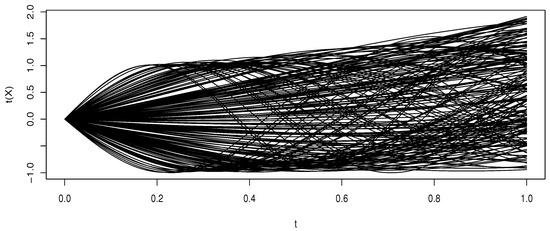
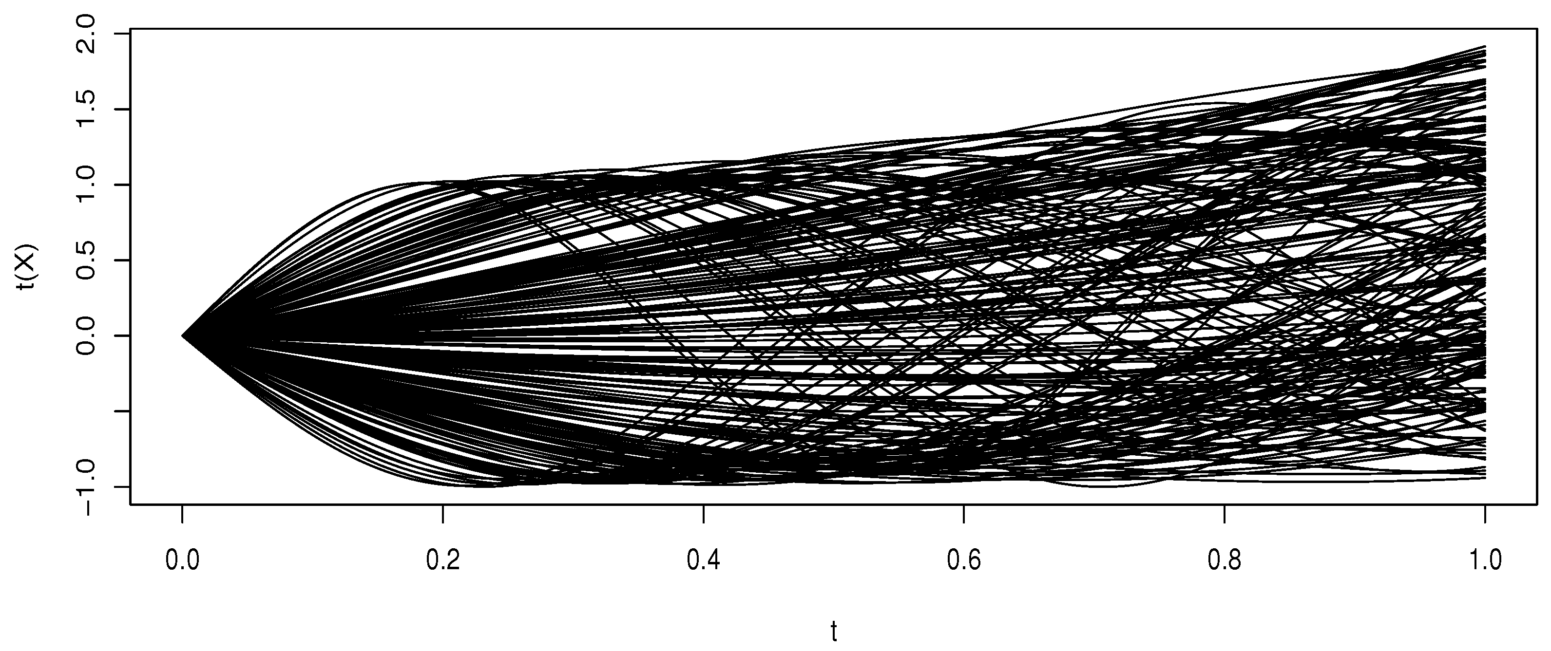
where the innovations are independent and identically distributed as and independent of the process . The initial state is drawn from . Subsequently, we simulate 200 independent variables , independent of the . For each pair , we define the functional covariates by
The functional variables are displayed in Figure 1.
Figure 1.
Sample trajectories , for and .
The response variables are generated from the nonparametric functional regression model
where the regression operator is specified as
with denoting the first derivative of , and where the errors satisfy independently. Following [29], the MAR mechanism is modeled through the conditional probability of observation:
where the logistic (expit) function is given by
and the scalar parameter controls the rate of missingness. The dependence between the functional covariate X and the missingness indicator thus varies with . For each simulated dataset, the empirical proportion of missing values is estimated by
In the simulation, and under assumption (H.6), we employ the Epanechnikov kernel:
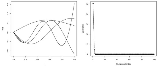
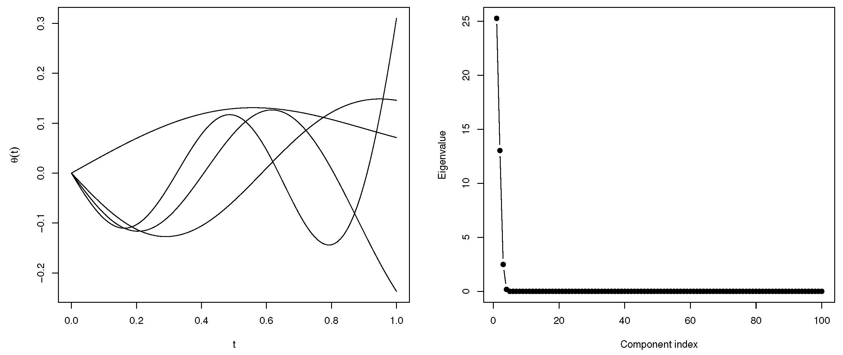
As previously discussed, the location functions and are chosen to reflect both the data structure and the smoothness of the functional trajectories. Specifically, we set
where is selected among the eigenfunctions of the empirical covariance operator
corresponding to the leading eigenvalues, with denoting the empirical mean function, see Figure 2.
Figure 2.
(Left): Eigenfunctions , with , for . (Right): Scree plot of the corresponding empirical eigenvalues.
The choice of the bandwidth parameter is of central importance in smoothing-based estimation. In line with the classical kernel regression framework (see [3]), the optimal bandwidth is determined via cross-validation:
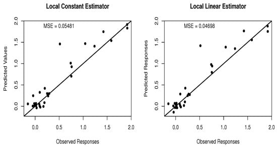
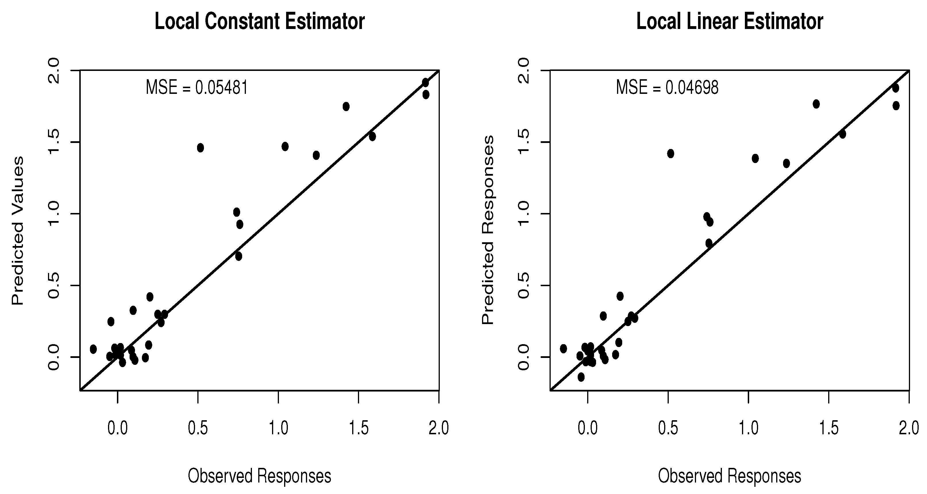
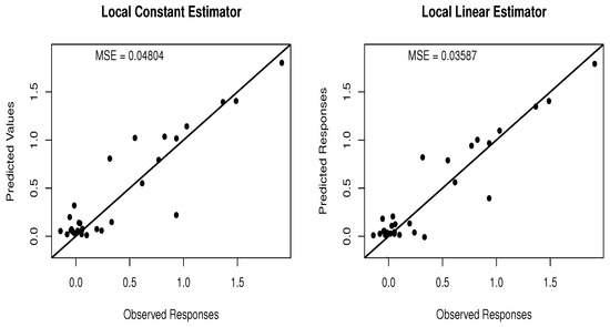
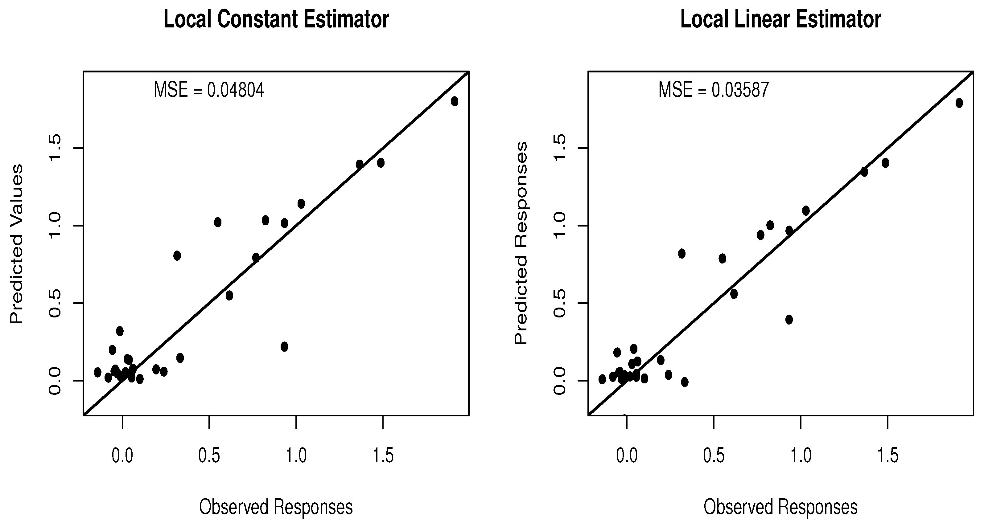
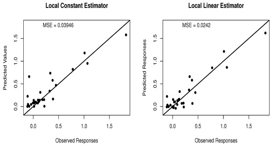
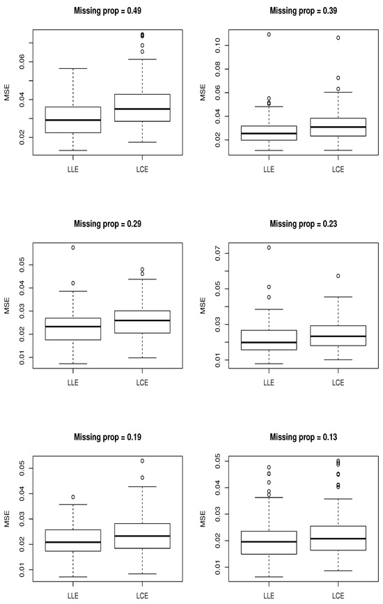
where denotes the leave-one-out estimator of the regression operator. To evaluate the influence of the parameter on predictive performance, we consider samples of size , partitioned into a training set of 170 observations and a test set of 30 observations. This splitting procedure is repeated 40 times for each value of . At each replication, the mean squared error (MSE) is computed for both estimators. The predictive accuracy is further assessed by plotting true versus predicted values and by computing the empirical MSE, defined as
Representative results are presented in Figure 3, Figure 4 and Figure 5.
Figure 3.
MSE of both estimators under MAR with .
Figure 4.
MSE of both estimators under MAR with .
Figure 5.
MSE of both estimators under MAR with .
From the results reported in Figure 3, Figure 4 and Figure 5, it follows that the local linear estimator (LLE) uniformly outperforms the local constant estimator (LCE) in terms of estimation accuracy. The performance of the LCE is markedly sensitive to the proportion of missing observations, thereby rendering it less reliable in the presence of incomplete data. In contrast, the LLE achieves a more favorable bias–variance trade-off (MSE), particularly under weak MAR mechanisms (i.e., for large values of ), where the attenuation of bias dominates the effect of the missingness. Consequently, the proposed procedure exhibits enhanced flexibility and improved fidelity to the underlying regression function. These findings are formally summarized in Table 1, which demonstrates a monotone increase in predictive accuracy as the fraction of missing data decreases. Furthermore, the LLE consistently exhibits superior finite-sample behavior relative to the LCE, with the performance differential being most striking for smaller values of , corresponding to higher levels of missingness.
Table 1.
Effect of on missing data proportion and prediction error (MSE) for the Local Constant Estimator (LCE) and the Local Linear Estimator (LLE).
To enhance the reliability and robustness of the proposed Locally Linear Estimator (LLE), we fixed the sample size at and examined several levels of missingness, expressed as different percentages of missing data. For each proportion , we performed 100 independent replications of the experiment. The performance of the proposed methodology was then systematically assessed across a range of complex regression models, using two widely adopted error metrics: the Mean Squared Error (MSE) and the Mean Absolute Percentage Error (MAPE).
The regression models considered below were carefully chosen to reflect distinct levels of structural complexity and nonlinearity in the regression relationship. Specifically, we investigated the following designs:
- M1.
- where the signal is expressed through the integrated derivative of the covariate trajectory.
- M2.
- with independent noise terms .
The predictive accuracy of the estimators was further quantified through the Mean Absolute Percentage Error (MAPE), defined, respectively, for the LLE and the Local Constant Estimator (LCE) as
The choice of both MSE and MAPE as performance measures is motivated by their complementary interpretive value. While the MSE penalizes large deviations more heavily and is therefore sensitive to outliers, the MAPE provides a scale-free measure that facilitates comparison across models with different magnitudes of response. Taken together, these criteria allow for a more comprehensive evaluation of the finite-sample behavior of the estimators.
In the following, we present the simulation results presenting the impact of the missing data mechanism on the performance of the proposed estimator in comparison with the local constant alternative. The overall performance, summarized by the mean values of the MSE and MAPE across 100 replications (denoted MMSE and MMAPE, respectively), is provided in Table 2.
Table 2.
Mean Squared Error (MMSE) and Mean Absolute Percentage Error (MMAPE) of the two estimators over 100 replications.
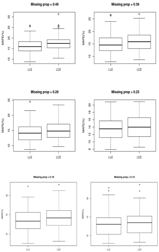
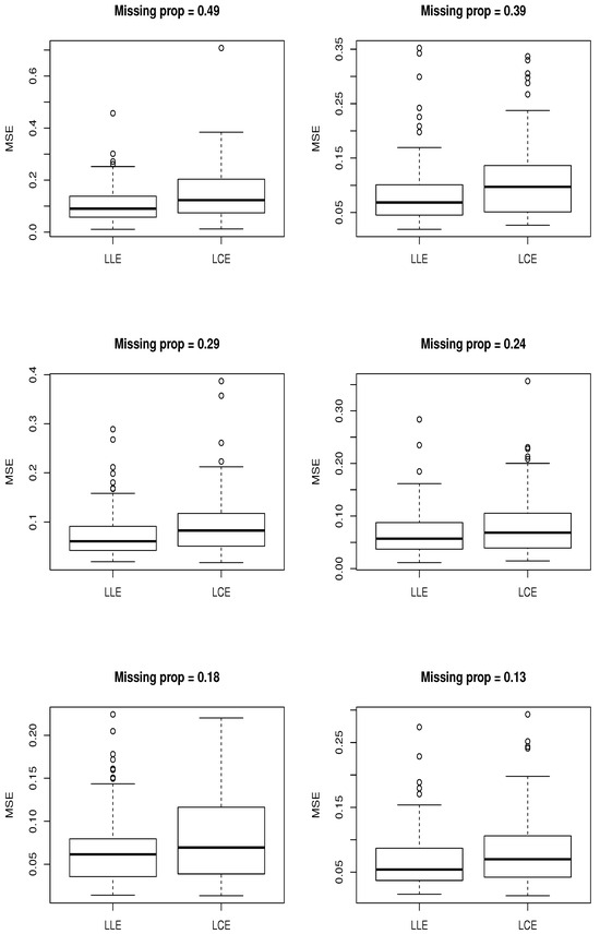
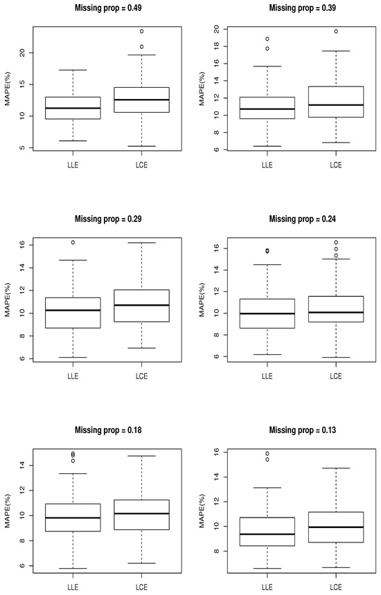
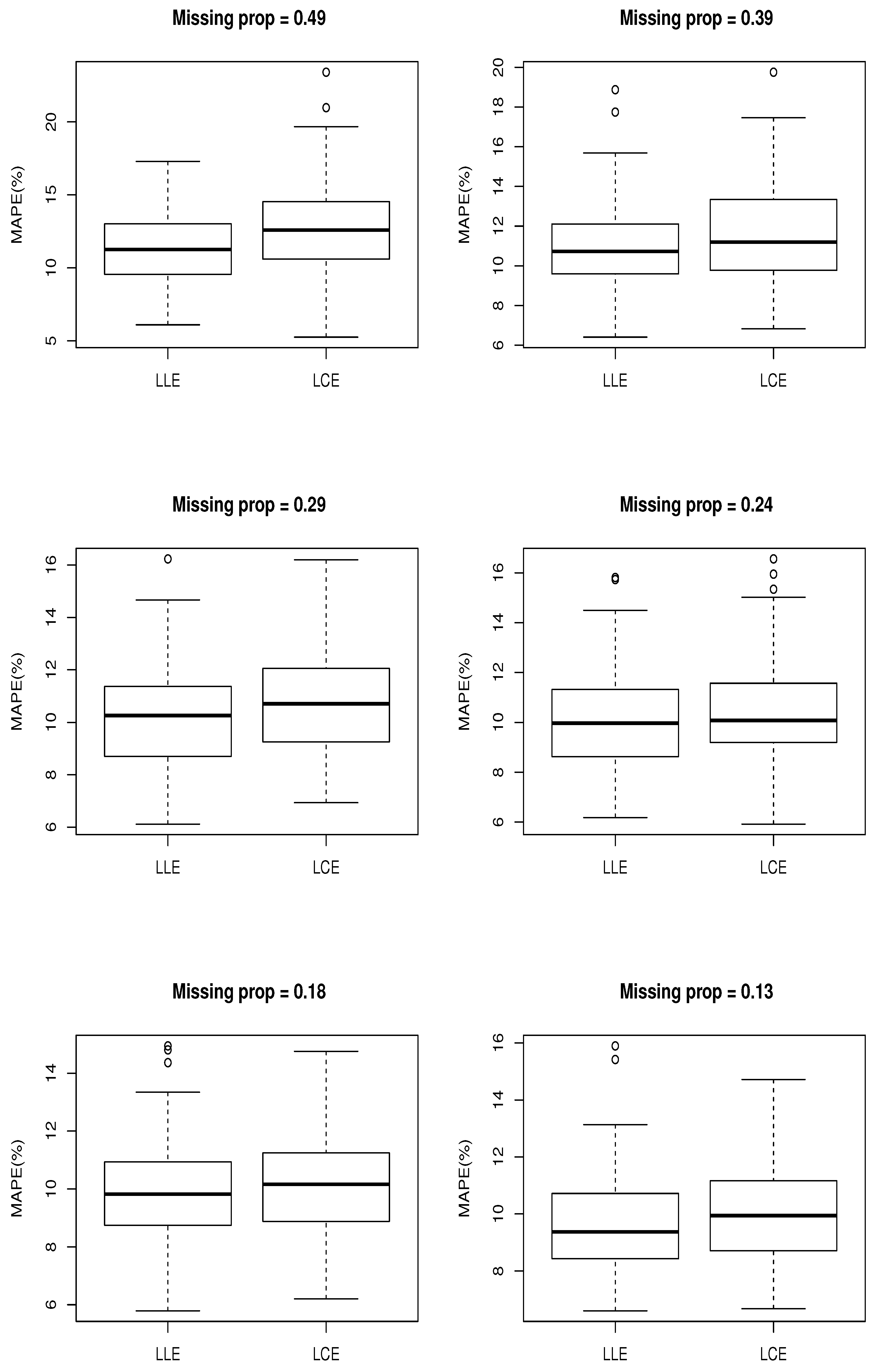
Figure 6, Figure 7, Figure 8 and Figure 9 display boxplot representations of the sampling distributions of the predictive performance measures associated with the estimator , computed over 100 independent replications. The comparison is carried out with respect to the response variable generated under models M1 and M2, and the evaluation is performed using two conventional accuracy criteria:
Figure 6.
Boxplots of the Mean Squared Error (MSE) Distributions for Both Estimators under the MAR Mechanism, Based on 100 Replications of Model M1.
Figure 7.
Boxplots of the empirical distribution of the Mean Absolute Percentage Error (MAPE) for both estimators under the Missing At Random (MAR) mechanism, based on 100 Monte Carlo replications using Model M1.
Figure 8.
Boxplots of the Empirical Distribution of the MSE for Both Estimators under the MAR Mechanism, Based on 100 Monte Carlo Replications Using Model M2.
Figure 9.
Boxplots of the empirical distribution of the Mean Absolute Percentage Error (MAPE) for the two estimators under the MAR mechanism, based on 100 replications from Model M2.
- The sampling distributions of the Mean Squared Error (MSE) and the Mean Absolute Percentage Error (MAPE) for , when estimated via the Local Linear Estimator (LLE), are reported in the panels on the left.
- The corresponding sampling distributions of the MSE and MAPE for , obtained through the Local Constant Estimator (LCE), are displayed in the panels on the right.
5. Concluding Remarks
In this article, we have developed a kernel-based estimation procedure for functional regression in the presence of missing responses, with particular attention to the MAR mechanism. Within the framework of stationary and ergodic functional processes, we introduced a local linear estimator of the regression operator and established its principal asymptotic properties. Specifically, we derived uniform almost sure convergence rates, established asymptotic normality, and provided explicit closed-form expressions for both the asymptotic bias and variance. Taken together, these results yield a rigorous and comprehensive asymptotic characterization of the proposed estimator under the MAR paradigm.
Several important theoretical and methodological directions remain open. A central unresolved issue concerns the optimal selection of the smoothing parameters. In kernel-based nonparametric estimation, bandwidth selection plays a decisive role in governing the bias–variance trade-off, thereby directly influencing the estimator’s risk profile. While the present study refrains from addressing this aspect, future work should focus on developing fully data-driven selection rules, such as cross-validation, plug-in approaches, penalized criteria, or multiscale adaptive methods, accompanied by a precise theoretical analysis of their asymptotic properties. Establishing minimax-optimal bandwidth selection procedures under MAR represents a particularly challenging, yet essential, research avenue.
A second limitation of the current framework lies in the assumption of strict stationarity. Although this assumption simplifies the asymptotic analysis, it may be unduly restrictive in empirical contexts characterized by temporal heterogeneity or structural evolution. Extending the methodology to locally stationary functional ergodic processes would permit the regression operator to evolve smoothly over time, thereby capturing a richer class of nonstationary dynamics. From a theoretical perspective, this extension would require the derivation of uniform laws of large numbers, central limit theorems, and strong approximation results in the locally stationary functional setting, where classical ergodic tools are no longer directly applicable.
Beyond these aspects, several additional perspectives merit attention. First, it is natural to inquire into the minimax efficiency of the proposed estimator. Establishing lower bounds for estimation under MAR mechanisms and determining whether the convergence rates achieved herein are sharp would provide a deeper understanding of the optimality properties of the procedure. Second, one may consider adaptive estimation strategies capable of accommodating heterogeneity in smoothness across the domain of the regression operator, for example via anisotropic kernels or locally adaptive bandwidths.
Another fertile line of investigation concerns the relaxation of the MAR assumption itself. Extending the framework to allow for Missing Not At Random (MNAR) mechanisms, where the probability of missingness depends explicitly on the unobserved responses, would represent a substantial generalization. Addressing this setting would likely require combining kernel-based functional regression techniques with tools from semiparametric efficiency theory, inverse-probability weighting, and possibly instrumental variable methods.
Finally, the advent of high-dimensional and large-scale functional data calls for the development of computationally efficient variants of the proposed methodology. Embedding the kernel estimators in reproducing kernel Hilbert space (RKHS) structures, employing random projection techniques, or leveraging sparsity and dimension reduction methods could provide avenues for scalability without sacrificing statistical rigor.
Author Contributions
Conceptualization, Y.B., O.B. and S.B.; methodology, Y.B., O.B. and S.B.; validation, Y.B., O.B. and S.B.; formal analysis, Y.B., O.B. and S.B.; investigation, Y.B., O.B. and S.B.; resources, Y.B., O.B. and S.B.; writing—original draft preparation, Y.B., O.B. and S.B.; writing—review and editing, Y.B., O.B. and S.B. All authors have read and agreed to the published version of the manuscript.
Funding
This research received no external funding.
Institutional Review Board Statement
Not applicable.
Informed Consent Statement
Not applicable.
Data Availability Statement
Data are contained within the article.
Acknowledgments
The authors extend their sincere gratitude to the Editor-in-Chief, the Associate Editor, and the three referees for their invaluable feedback and for pointing out a number of oversights in the version initially submitted. Their insightful comments have greatly refined and focused the original work, resulting in a markedly improved presentation.
Conflicts of Interest
The authors declare that they have no known competing financial interests or personal relationships that could have appeared to influence the work reported in this paper.
Appendix A
We begin by presenting several preliminary technical lemmas that will be instrumental in obtaining our asymptotic results.
Lemma A1.
Let assumptions (H.4), (H.6), and (H.8) hold. Then, for and , the following conditional moment expansions are valid:
Remark A1.
Provided that conditions (H.1) and (H.2) are satisfied, the assertion of Lemma A1 is valid uniformly for all .
Lemma A2.
Suppose that assumptions (H.1), (H.2), (H.5-ii), (H.6), and (H.8) hold. Then, in conjunction with Lemma A1, the following assertions are valid:
Proof of Lemma A1.
(a) By combining the property of conditional expectation with the condition characterizing missing data at random (MAR), for , we can write
(b) For all , the following holds under assumption (H.6):
Therefore, applying Assumption (H.8-ii) yields
which immediately implies
(c) Since the variables and Y are independent given , we have
By applying the conditional Cauchy–Schwarz inequality, we obtain
Furthermore, we have
Alternatively, under Assumptions (H.4) and (H.6), we establish the following result:
Using Lemma A1, we deduce that
(d)
Let and ; we can write
where
Moreover, under assumption (H4-ii), we have
Hence the proof is complete. □
Proof of Lemma A2.
By invoking part (c) of Lemma A1, with specified as the trivial -algebra, and subsequently applying Lemma A.1 of [35], under assumption (H.1), we deduce that
Applying Lemma A1, under the standing assumptions (H.2) and (H.5), we obtain the following result:
Consequently, we arrive at the following uniform bound:
Moreover, recalling that the inequality holds for all , it follows that
Since almost completely as a consequence of assumption (H.2-ii), we deduce that there exists a strictly positive constant C such that
This inequality ensures the validity of the required bound, thereby establishing the claim and completing the proof. □
Proof of Lemma 1.
Proof of Lemma 2.
Building upon (6), we rigorously establish the uniform convergence of our estimator over a subset . For this purpose, we define
For we have
We now turn to the analysis of the term . Exploiting the boundedness property of K, this term can be expressed as as follows:
By applying inequality (A8), we obtain
We begin by examining the term . Under assumption (H.6), and invoking the bound
the quantity can be decomposed into the sum of the following three components:
with
Since the kernel K is Lipschitz continuous on the interval in this setting, it immediately follows that
Under assumption (H.3), we have
which implies that
By invoking the exponential inequality for unbounded random variables (cf. [3], Corollary A.8), and selecting we deduce that
It suffices to combine the conditions (H.1) and (H.7) to obtain
Following the same approach used for , one can write
where
Under assumptions (H.1) and (H.3), we have
By invoking the exponential inequality for unbounded random variables and selecting the parameter we obtain the following result:
We now analyze the term . Using the same decomposition as used for , we have
where
Concerning , we have
Therefore, we obtain
where
We put
We consider the following decomposition:
where
and
Under assumption (H.4) for all , we have
This implies that, for we obtain
and
However, in the case and , we obtain
Combining (A10) and (A11), we find that
Then, by assumption (H.6), we obtain
Following the same idea used in the proof of , we obtain
Concerning the term , for all , we have
However, we can write
where is a martingale difference. Consequently, Lemma A3 can be invoked to establish an exponential upper bound for the quantity . To this end, we verify the conditions under which such an exponential bound can be obtained. Thereafter, applying Jensen’s inequality yields
From Lemma A1 and inequality (A6), it follows that
We take
Thus, for any we have
Making use of the statement (A8), we have
Using assumptions (H.2-ii) and (H.8), we deduce that
Then, we derive
Thus, by choosing such that , we get
Since
we obtain that
Concerning the term of it is obvious that
and we infer that
Hence, the proof is complete. □
Proof of Lemma 3.
According to the inequality of (A9), we have
meaning that there exists such that
Taking as a trivial algebra in Lemma 2, we deduce that there exists
such that
Hence, the proof is concluded. □
Proof of Lemma 4.
We have the following decomposition:
where
The primary objective is to establish that
We denote
Thus, the sequence naturally arises as a triangular array of martingale difference terms adapted to the filtration . Note that
On the other hand, by appealing to Burkholder’s inequality for martingale difference sequences [55], it follows that
By invoking inequality (A8) and considering as the trivial -algebra in (A13), we consequently obtain that
Secondly, we will prove that
By invoking the sufficient condition for convergence in probability, it remains only to establish the following results:
We have
Note that
By applying Lemma A1, we obtain
Under assumption (H.8), we deduce that
Hence, the proof is complete. □
Proof of Lemma 5.
We denote
We define . It is clear that
Moreover, to prove Lemma 5, it suffices to establish the following two statements:
and
Concerning the proof of (A15), we have
For the second term on the right-hand side of Equation (A17), we use Lemma 1 and the statement (A8) to conclude that
Moreover,
Then
Under assumption (H.2), we obtain
In order to establish the statement (A16), we consider the following decomposition:
where
and
By the properties of conditional expectations, we obtain
Then, we have
Combining assumption B(2) and Lemma A1 with Lemma. A.2 (ii) of [56], we get
By the assumptions (H.2) and (H.4), and using the statements (A13) and (A8), we obtain
Concerning Equation (A16), for all , we have
Let and such that
By Hölder and Markov inequalities, one can write for all ,
Let for any such that
is a continuous function. It follows that
This completes the proof. □
Appendix B
This appendix presents supplementary material that is integral to developing a more thorough and nuanced understanding of the paper’s contributions. In contexts involving dependent data—particularly under ergodicity—martingale difference sequences (MDSs) emerge as a central analytical framework. The derivation of general results for MDS is essential for investigating the asymptotic properties of a wide class of statistics, stochastic processes, and estimators that can be represented in terms of these sequences.
Definition A1.
Let be a filtration (an increasing sequence of σ algebras), and let be a sequence of integrable random variables with real values adapted to . The sequence is called a martingale difference sequence (MDS) with respect to if, for all ,
In the asymptotic analysis of our estimators for functional ergodic data, rigorous control of the deviation probabilities associated with partial sums of unbounded martingale differences is of critical importance. The lemma below establishes an exponential deviation bound for these partial sums, under a suitable moment growth condition.
Lemma A3
(Exponential Bound for Martingale Partial Sums). Let be a martingale difference sequence with respect to its natural filtration. Suppose there exist constants and a sequence such that, for all ,
Then, for any ,
where
Theorem A1
(Lindeberg central limit theorem). Let be a triangular array of independent random variables for each , satisfying
Define the normalized variables
Then the sum of the normalized variables converges in distribution to the standard normal distribution:
provided the following Lindeberg condition holds: for every ,
References
- Bosq, D. Linear Processes in Function Spaces; Lecture Notes in Statistics; Theory and Applications; Springer: New York, NY, USA, 2000; Volume 149, p. xiv+283. [Google Scholar] [CrossRef] [Scilit]
- Ramsay, J.O.; Silverman, B.W. Functional Data Analysis, 2nd ed.; Springer Series in Statistics; Springer: New York, NY, USA, 2005; p. xx+426. [Google Scholar] [CrossRef] [Scilit]
- Ferraty, F.; Vieu, P. Nonparametric Functional Data Analysis; Springer Series in Statistics; Theory and Practice; Springer: New York, NY, USA, 2006; p. xx+258. [Google Scholar] [CrossRef] [Scilit]
- Horváth, L.; Kokoszka, P. Inference for Functional Data with Applications; Springer Series in Statistics; Springer: New York, NY, USA, 2012. [Google Scholar] [CrossRef] [Scilit]
- Zhang, J. Analysis of Variance for Functional Data; Monographs on Statistics and Applied Probability; CRC Press: Boca Raton, FL, USA, 2014; Volume 127. [Google Scholar] [CrossRef] [Scilit]
- Qing, S.; Choi, T. Gaussian Process Regression Analysis for Functional Data; CRC Press: Boca Raton, FL, USA, 2011. [Google Scholar] [CrossRef] [Scilit]
- Goia, A.; Vieu, P. A partitioned single functional index model. Comput. Statist. 2015, 30, 673–692. [Google Scholar] [CrossRef] [Scilit]
- Chen, D.; Hall, P.; Müller, H. Single and Multiple Index Functional Regression Models with Nonparametric Link. Ann. Stat. 2011, 39, 1720–1747. [Google Scholar] [CrossRef] [Scilit]
- Aneiros, G.; Vieu, P. Partial linear modelling with multi-functional covariates. Comput. Statist. 2015, 30, 647–671. [Google Scholar] [CrossRef] [Scilit]
- Ferré, L.; Yao, A.F. Smoothed functional inverse regression. Statist. Sin. 2005, 15, 665–683. [Google Scholar]
- Horváth, L.; Rice, G. An introduction to functional data analysis and a principal component approach for testing the equality of mean curves. Rev. Mat. Complut. 2015, 28, 505–548. [Google Scholar] [CrossRef] [Scilit]
- Müller, H. Peter Hall, functional data analysis and random objects. Ann. Statist. 2016, 44, 1867–1887. [Google Scholar] [CrossRef] [Scilit]
- Ling, N.; Vieu, P. Nonparametric modelling for functional data: Selected survey and tracks for future. Statistics 2018, 52, 934–949. [Google Scholar] [CrossRef] [Scilit]
- Goia, A.; Vieu, P. An introduction to recent advances in high/infinite dimensional statistics [Editorial]. J. Multivar. Anal. 2016, 146, 1–6. [Google Scholar] [CrossRef] [Scilit]
- Bouzebda, S. Weak convergence of the conditional single index U-statistics for locally stationary functional time series. AIMS Math. 2024, 9, 14807–14898. [Google Scholar] [CrossRef] [Scilit]
- Masry, E. Multivariate regression estimation—Local polynomial fitting for time series. Stoch. Process. Appl. 1996, 65, 81–101. [Google Scholar] [CrossRef] [Scilit]
- Masry, E. Multivariate regression estimation of continuous-time processes from sampled data: Local polynomial fitting approach. IEEE Trans. Inform. Theory 1999, 45, 1939–1953. [Google Scholar] [CrossRef]
- Masry, E. Multivariate local polynomial regression for time series: Uniform strong consistency and rates. J. Time Ser. Anal. 1996, 17, 571–599. [Google Scholar] [CrossRef] [Scilit]
- Masry, E.; Fan, J. Local polynomial estimation of regression functions for mixing processes. Scand. J. Statist. 1997, 24, 165–179. [Google Scholar] [CrossRef] [Scilit]
- Masry, E.; Mielniczuk, J. Local linear regression estimation for time series with long-range dependence. Stoch. Process. Appl. 1999, 82, 173–193. [Google Scholar] [CrossRef] [Scilit]
- Wu, J.; Peng, H.; Tu, W. Large-sample estimation and inference in multivariate single-index models. J. Multivar. Anal. 2019, 171, 382–396. [Google Scholar] [CrossRef] [Scilit]
- Cheng, P.E. Nonparametric estimation of mean functionals with data missing at random. J. Am. Stat. Assoc. 1994, 89, 81–87. [Google Scholar] [CrossRef]
- Little, R.J.A.; Rubin, D.B. Statistical Analysis with Missing Data, 2nd ed.; Wiley Series in Probability and Statistics; Wiley-Interscience [John Wiley & Sons]: Hoboken, NJ, USA, 2002; p. xviii+381. [Google Scholar] [CrossRef] [Scilit]
- Nittner, T. Missing at random (MAR) in nonparametric regression—A simulation experiment. Stat. Methods Appl. 2003, 12, 195–210. [Google Scholar] [CrossRef] [Scilit]
- Wang, Q.; Linton, O.; Härdle, W. Semiparametric regression analysis with missing response at random. J. Amer. Statist. Assoc. 2004, 99, 334–345. [Google Scholar] [CrossRef] [Scilit]
- Liang, H.; Wang, S.; Carroll, R.J. Partially linear models with missing response variables and error-prone covariates. Biometrika 2007, 94, 185–198. [Google Scholar] [CrossRef] [Scilit]
- Efromovich, S. Nonparametric regression with predictors missing at random. J. Amer. Statist. Assoc. 2011, 106, 306–319. [Google Scholar] [CrossRef] [Scilit]
- Josse, J.; Reiter, J.P. Introduction to the special section on missing data. Statist. Sci. 2018, 33, 139–141. [Google Scholar] [CrossRef] [Scilit]
- Ferraty, F.; Sued, M.; Vieu, P. Mean estimation with data missing at random for functional covariables. Statistics 2013, 47, 688–706. [Google Scholar] [CrossRef] [Scilit]
- Ling, N.; Liang, L.; Vieu, P. Nonparametric regression estimation for functional stationary ergodic data with missing at random. J. Statist. Plann. Inference 2015, 162, 75–87. [Google Scholar] [CrossRef] [Scilit]
- Febrero-Bande, M.; Galeano, P.; González-Manteiga, W. Estimation, imputation and prediction for the functional linear model with scalar response with responses missing at random. Comput. Statist. Data Anal. 2019, 131, 91–103. [Google Scholar] [CrossRef] [Scilit]
- Kraus, D. Inferential procedures for partially observed functional data. J. Multivar. Anal. 2019, 173, 583–603. [Google Scholar] [CrossRef] [Scilit]
- Bouanani, O.; Bouzebda, S. Limit theorems for local polynomial estimation of regression for functional dependent data. AIMS Math. 2024, 9, 23651–23691. [Google Scholar] [CrossRef] [Scilit]
- Baíllo, A.; Grané, A. Local linear regression for functional predictor and scalar response. J. Multivar. Anal. 2009, 100, 102–111. [Google Scholar] [CrossRef] [Scilit]
- Barrientos-Marin, J.; Ferraty, F.; Vieu, P. Locally modelled regression and functional data. J. Nonparametr. Stat. 2010, 22, 617–632. [Google Scholar] [CrossRef] [Scilit]
- Kolmogorov, A.N.; Tihomirov, V.M. ε-entropy and ε-capacity of sets in function spaces. Uspehi Mat. Nauk 1959, 14, 3–86. [Google Scholar]
- Bouzebda, S.; Nezzal, A. Uniform in number of neighbors consistency and weak convergence of kNN empirical conditional processes and kNN conditional U-processes involving functional mixing data. AIMS Math. 2024, 9, 4427–4550. [Google Scholar] [CrossRef] [Scilit]
- Ferraty, F.; Laksaci, A.; Tadj, A.; Vieu, P. Rate of uniform consistency for nonparametric estimates with functional variables. J. Statist. Plann. Inference 2010, 140, 335–352. [Google Scholar] [CrossRef] [Scilit]
- Kuelbs, J.; Li, W.V. Metric entropy and the small ball problem for Gaussian measures. J. Funct. Anal. 1993, 116, 133–157. [Google Scholar] [CrossRef] [Scilit]
- Nicoleris, T.; Yatracos, Y.G. Rates of convergence of estimates, Kolmogorov’s entropy and the dimensionality reduction principle in regression. Ann. Statist. 1997, 25, 2493–2511. [Google Scholar] [CrossRef] [Scilit]
- Li, W.V.; Shao, Q.M. Gaussian processes: Inequalities, small ball probabilities and applications. In Handbook of Statistics, Stochastic Processes: Theory and Methods; Elsevier: Amsterdam, The Netherlands, 2001; Volume 19, pp. 533–597. [Google Scholar] [CrossRef] [Scilit]
- Laib, N.; Louani, D. Nonparametric kernel regression estimation for functional stationary ergodic data: Asymptotic properties. J. Multivar. Anal. 2010, 101, 2266–2281. [Google Scholar] [CrossRef] [Scilit]
- Litimein, O.; Alshahrani, F.; Bouzebda, S.; Laksaci, A.; Mechab, B. Kolmogorov Entropy for Convergence Rate in Incomplete Functional Time Series: Application to Percentile and Cumulative Estimation in High Dimensional Data. Entropy 2023, 25, 1108. [Google Scholar] [CrossRef] [Scilit]
- Rosenblatt, M. Uniform ergodicity and strong mixing. Z. Wahrscheinlichkeitstheorie und Verw. Gebiete 1972, 24, 79–84. [Google Scholar] [CrossRef] [Scilit]
- Bouzebda, S.; Didi, S. Multivariate wavelet density and regression estimators for stationary and ergodic discrete time processes: Asymptotic results. Comm. Statist. Theory Methods 2017, 46, 1367–1406. [Google Scholar] [CrossRef] [Scilit]
- Bouzebda, S.; Didi, S. Some asymptotic properties of kernel regression estimators of the mode for stationary and ergodic continuous time processes. Rev. Mat. Complut. 2021, 34, 811–852. [Google Scholar] [CrossRef] [Scilit]
- Bradley, R.C. Introduction to Strong Mixing Conditions, Vol. 3; Kendrick Press: Heber City, UT, USA, 2007; p. xii+597. [Google Scholar]
- Leucht, A.; Neumann, M.H. Degenerate U- and V-statistics under ergodicity: Asymptotics, bootstrap and applications in statistics. Ann. Inst. Statist. Math. 2013, 65, 349–386. [Google Scholar] [CrossRef] [Scilit]
- Neumann, M.H. Absolute regularity and ergodicity of Poisson count processes. Bernoulli 2011, 17, 1268–1284. [Google Scholar] [CrossRef] [Scilit]
- Chaouch, M.; Laïb, N. Regression estimation for continuous-time functional data processes with missing at random response. J. Nonparametr. Stat. 2025, 37, 1–32. [Google Scholar] [CrossRef] [Scilit]
- Giraitis, L.; Leipus, R. A generalized fractionally differencing approach in long-memory modeling. Liet. Mat. Rink. 1995, 35, 65–81. [Google Scholar] [CrossRef] [Scilit]
- Guégan, D.; Ladoucette, S. Non-mixing properties of long memory processes. C. R. Acad. Sci. Paris Sér. I Math. 2001, 333, 373–376. [Google Scholar] [CrossRef] [Scilit]
- Andrews, D.W.K. Non-strong mixing autoregressive processes. J. Appl. Probab. 1984, 21, 930–934. [Google Scholar] [CrossRef] [Scilit]
- Francq, C.; Zakoïan, J.M. GARCH Models; Structure, Statistical Inference and Financial Applications; John Wiley & Sons, Ltd.: Chichester, UK, 2010; p. xiv+489. [Google Scholar] [CrossRef] [Scilit]
- Hall, P.; Heyde, C.C. Martingale Limit Theory and Its Application; Academic Press: Cambridge, MA, USA, 1980. [Google Scholar] [CrossRef] [Scilit]
- Ayad, S.; Laksaci, A.; Rahmani, S.; Rouane, R. Local linear modelling of the conditional distribution function for functional ergodic data. Math. Model. Anal. 2022, 27, 360–382. [Google Scholar] [CrossRef] [Scilit]

Disclaimer/Publisher’s Note: The statements, opinions and data contained in all publications are solely those of the individual author(s) and contributor(s) and not of MDPI and/or the editor(s). MDPI and/or the editor(s) disclaim responsibility for any injury to people or property resulting from any ideas, methods, instructions or products referred to in the content. |
© 2025 by the authors. Licensee MDPI, Basel, Switzerland. This article is an open access article distributed under the terms and conditions of the Creative Commons Attribution (CC BY) license (https://creativecommons.org/licenses/by/4.0/).