Numerical Tests of Formulae for Volume Enclosed by Flux Surfaces of Integrable Magnetic Fields

Abstract

Numerical tests of volume formulae are presented to efficiently compute the volume enclosed between flux surfaces for integrable 3D vector fields with various degrees of symmetry. In the process, a new case is proposed and tested.

1. Introduction

In the design of magnetic confinement devices for plasma, it is often important to determine the volume V enclosed by a flux surface S, particularly the volume bounded by the outermost flux surface of a given class within the vacuum vessel. This is one objective function that is considered in computational optimisation of designs, e.g., [1]. Given the field, the volume is usually found by simple 3D integration.

An approach presented in [2] derives expressions for the volume that take advantage of the invariance of S under the magnetic field B for a range of integrable cases, thereby simplifying the conventional three-dimensional integration and potentially enabling more efficient computation.

The purpose of this work is to test the volume formulae in [2] numerically on relevant, non-trivial examples, in order to demonstrate the advantages or potential issues arising from their use.

The explicit example fields available for numerical testing are rather limited, as these formulae require some form of integrability, in particular the existence of a continuous family of flux surfaces and an associated label function $\mathsf{\Psi }$, so we restrict our attention to example fields that are integrable. This is, however, a common assumption in the plasma physics context, e.g., [3], because it holds for all non-degenerate magnetohydrostatic (MHS) fields (MHS means $J\times B=\nabla p$ for some function p, where $J=\mathrm{curl}B$, and non-degenerate means $\nabla p\ne 0$ except on a set of measure zero). It is also a common assumption in numerical codes for computing MHS fields and more generally MHD equilibria (but see Ref. [4] for one that does not make this assumption and presents references to various ones that do).

Section 2.1 provides a brief exposition of the terminology and results from [2], plus a new result that treats the case of integrable magnetic fields for which the associated symmetry preserves some density that is not necessarily constant. Section 2.2 describes the analytical magnetic fields used to test these results. Section 3 presents our numerical findings, which are discussed in Section 4, and the conclusions are summarised in Section 5.

2. Materials and Methods

2.1. Volume Enclosed by Flux Surfaces

A magnetic field is a $C^1$ vector field B on an orientable three-dimensional manifold M that preserves a volume form Ω (for the standard Euclidean volume, this is the condition $\mathrm{div}B=0$).

We will formulate most of our exposition in the language of exterior calculus because it makes many concepts much simpler to express and some results more evident. It is less familiar to plasma physicists, however, to whom this work is particularly directed, so we translate into vector calculus language in many places.

In the language of exterior calculus, to a magnetic field B, an associated flux 2-form can be defined as $\beta =i_B\mathrm{\Omega }$, allowing the volume-preservation condition to be written as $d\beta =0$ (i.e., $\beta$ is closed: its integral over any closed surface contractible to a point is zero). The vector calculus interpretation of $\beta$ is that acting on a pair of vectors $\xi$ and $\eta$, $\beta (\xi ,\eta )=B·dS$ for the area element $dS$ given by the oriented parallelogram spanned by $\xi$ and $\eta$. So $\beta$ can be integrated over a surface S by chopping S into little parallelograms, summing their contributions and taking the limit. The exterior derivative $d\beta$ of $\beta$ is defined to be the 3-form, acting on oriented triples of vectors, that gives the sum of $\beta$ over the faces of the parallelepiped they span, oriented outwards. The exterior derivative d on 1-forms is defined similarly, and on functions $f:{\mathbb{R}}^3\to \mathbb{R}$, $df$ is just the ordinary derivative. A tutorial on the use of differential forms in plasma physics can be found in [5].

The fields relevant to the present work, and to much of plasma physics, typically assume the slightly stronger condition that $\beta$ is exact, i.e., $\beta =d\alpha$ for some 1-form $\alpha$. This is equivalent to requiring the existence of a vector potential A such that $B=\nabla \times A$, where $\alpha =A^{♭}$, the 1-form that when acting on any vector $\xi$ produces $A^{♭}\left(\xi \right)=A·\xi$. Another way to define exactness of $\beta$ is that ${\int }_S\beta =0$ for any closed surface S, not only contractible ones.

An invariant torus of B is called a flux surface. A magnetic field is called integrable if there is a $C^1$ function $\mathrm{\Psi }$ (called a flux function or flux surface label) such that $d\mathrm{\Psi }\ne 0$ almost everywhere (a.e.) and $i_{B}d\mathrm{\Psi }=0$ (in vector calculus, $\nabla \mathrm{\Psi }\ne 0$ a.e. and $B·\nabla \mathrm{\Psi }=0$, but the property does not require the Riemannian metric implicit in ∇ and ·, which is why we prefer to express it using differential forms). For an integrable field, the level sets of $\mathrm{\Psi }$ are invariant under B. If B and $d\mathrm{\Psi }$ are nowhere-zero on a compact component of a level set, then it is a torus and hence a flux surface. Furthermore, it has a neighbourhood that is foliated by flux surfaces. From KAM theory, if B is non-integrable but smooth enough, then various simple conditions imply a set of positive volumes of flux surfaces, but we will not be using that here.

To quantify the volume V enclosed by a flux surface S, once the surface has been computed, the enclosed volume can be obtained via a 3D integral ${\int }_V\mathrm{\Omega }$. This can be reduced to a 2D integral ${\int }_S\nu$ for some 2-form $\nu$ if the manifold M is contractible (i.e., $\mathrm{\Omega }=d\nu$ for some 2-form $\nu$ and then the result follows by Stokes’ theorem). For example, if $\mathrm{\Omega }=dx\wedge dy\wedge dz$, as for a standard volume in Cartesian coordinates, then one can take $\nu =zdx\wedge dy$, and integrating this over a closed surface corresponds to integrating the height difference between the points of the surface above a given point $(x,y)$ of the horizontal plane, with respect to horizontal area. However, this direct approach does not take into account the invariance of S under B.

The first formula presented in [2] for computing the volume that exploits this invariance is:

$$V={\int }_D\mathsf{T}\beta ,$$

(1)

where D is a disk transverse to B whose boundary is on the flux surface S, and $\mathsf{T}$ is the first-return time to D along the fieldline flow $\dot{x}=B\left(x\right)$. Although (1) is a 2D integral, it involves computing the return-time function, which effectively makes the integration 3D, so there is no real computational reduction (in the Appendix A, however, a way to reduce the computation of V from (1) as a function of $\mathrm{\Psi }$ for integrable fields is given).

So we are restricted to a sequence of special cases of magnetic field, for which the integration can be reduced. In the two strongest cases, it is reduced to 2D; in the other two cases, it is reduced to a bit more than 2D, in a sense to be described.

All cases considered are integrable, but they differ in their degree of symmetry. To explain this, note that if B is integrable and non-zero a.e., then there is a vector field u independent of B a.e. such that $L_u\beta =0$, where $L_u$ denotes the Lie derivative along u, that is, u is a symmetry of $\beta$. The expression of this in vector calculus language is $\mathrm{curl}(B\times u)+\left(\mathrm{div}B\right)u=0$. For example, if B is integrable (and divergence-free, always assumed), with flux function $\mathrm{\Psi }$, one can take $u=B\times \nabla \mathrm{\Psi }/{\left|B\right|}^2+fB$ using any Riemannian metric and any function f. But there might be values of u which preserve more than just $\beta$. For example, u might also preserve $\rho \mathrm{\Omega }$ ($L_u\left(\rho \mathrm{\Omega }\right)=0$, equivalently $\mathrm{div}\left(\rho u\right)=0$) for some positive function $\rho$, which we call a density. Or it might preserve volume $\mathrm{\Omega }$ (so constant density, $\mathrm{div}u=0$); in which case, $L_{u}B$ is also zero (it is equal to the commutator $[u,B]$, which can be written as $\mathrm{curl}(B\times u)-\mathrm{div}uB+\mathrm{div}Bu$). If in addition u preserves $\left|B\right|$ ($L_u\left|B\right|=0$, equivalently, $u·\nabla \left|B\right|=0$), then we say u is a weak quasisymmetry of B, or it might furthermore preserve $B^{♭}$ (defined the same way as $A^{♭}$), at which point we say u is a quasisymmetry of B (in vector calculus, $L_u{B}^{♭}=0$ is written as $\left(\mathrm{curl}B\right)\times u+\nabla (u·B)=0$).

Note that for an integrable field, it makes sense to ask to compute not just the volume enclosed by one flux surface, but instead the whole function giving the volume $V\left(\mathrm{\Psi }\right)$ enclosed as a function of $\mathrm{\Psi }$. Our methods will compute this by finding $dV/d\mathrm{\Psi }$ as a 1D integral (or a bit more) and then the function $V\left(\mathrm{\Psi }\right)$ by one more integration.

The proof of (1), as well as those of Theorems 1–4, can be found in [2]. A subsection on a new result, Theorem 3’, and its proof, is included.

In contrast to what we have just described, we will now treat the cases in order of decreasing specialisation.

2.1.1. Quasisymmetric Fields

A quasisymmetric (QS) magnetic field B is the special case in which there exists a vector field u independent from B almost everywhere (in the region of interest), with 

$$L_u\beta =0,L_u\mathrm{\Omega }=0,L_u{B}^{♭}=0.$$

(2)

Expressions for these in vector calculus language were given above. Under mild additional conditions [6], every orbit of u is closed and has the same period $\tau >0$.

The only known analytic examples of these fields (with bounded u orbits) are axisymmetric, where $u={\partial }_{\varphi }$ in cylindrical coordinates (the vector field with $\dot{\varphi }=1,\dot{r}=0,\dot{z}=0$) (so $\tau =2\pi$). It is an open question whether there are any other exactly quasisymmetric fields, although fields with non-axisymmetric quasisymmetry can be constructed to a high degree of accuracy [7].

The conditions $L_u\beta =0$ and $L_u\mathrm{\Omega }=0$ imply that $i_u\beta$ is a closed form, i.e., ${\int }_{\gamma }B\times u·dl$, and, along a path, $\gamma$ is unchanged under continuous deformation of the path preserving the ends. Assuming there is no homological obstruction (one might want to assume that every loop is contractible to a point but is stronger than necessary and rules out toroidal geometry; it is enough to suppose that each homology class in dimension 1 can be realised by an orbit of some linear combination of u and B), this further implies that $i_u\beta$ is exact; i.e., there exists a function $\mathrm{\Psi }$ such that $i_u\beta =d\mathrm{\Psi }$ ($B\times u=\nabla \mathrm{\Psi }$). It follows that both u and B are tangent to the level sets of $\mathrm{\Psi }$, $\mathrm{\Psi }$ is a flux or a label function, and that the bounded components of the level sets are tori.

Using the volume-preserving property and the conditions in (2), ref. [2] provides the following formula. Choose a u-line $\gamma$ and a point $x\in \gamma$, then

Theorem 1.

$dV=\tau T\left(\mathrm{\Psi }\right)d\mathrm{\Psi }$, where the return time $T>0$ is the first time for which the flow of B starting at x returns to γ.

• The return time can be proved to depend on x through only $\mathrm{\Psi }\left(x\right)$. As computing the return time $T\left(\mathrm{\Psi }\right)$ requires a 1D integration, the entire volume calculation is thereby reduced to a 2D integral. For clarity, the return time $T\left(\mathrm{\Psi }\right)$ corresponds to the time between two successive crossings of a fieldline on S with a u-line $\gamma$, while $\mathsf{T}$ in (1) corresponds to the time between two crossings through a given transverse disk D.

This result generalises to the case of a magnetic field with weak quasisymmetry [8]; this is defined by requiring

$$L_u\beta =0,L_u\mathrm{\Omega }=0,L_u\left|B\right|=0.$$

(3)

The only relevant consequence for the volume formula is that now the value of $\tau$ is in general a function of $\mathrm{\Psi }$. The extended result is the following:

Theorem 2.

$dV=\tau \left(\mathrm{\Psi }\right)T\left(\mathrm{\Psi }\right)d\mathrm{\Psi }$.

• Thus, the computation of the volume is still equivalent to a 2D integration. It is an open question again, however, whether there are any weak QS fields that are not axisymmetric.

2.1.2. Fields with Flux-Form Symmetry

The next case considered in [2] is magnetic fields B with flux-form symmetry, defined as having a volume-preserving vector field u independent from B almost everywhere, such that $L_u\beta =0$ (recall, this means $\mathrm{curl}(B\times u)=0$ because we are assuming $\mathrm{div}B=0$). Perhaps the name is insufficiently clear, because for the definition it is essential that u be volume-preserving, not just $L_u\beta =0$, but we continue to use it. It is equivalent to require u to be a volume-preserving field that commutes with B (e.g., [6]). It holds for all non-degenerate MHS fields that $u=J$, though all examples that we know of such fields are axisymmetric (so are already covered by Theorem 1).

Under the same homological condition, this implies again that $i_u\beta =d\mathrm{\Psi }$ for some function $\mathrm{\Psi }$ whose level sets are invariant under both u and B. Furthermore, the commutation condition implies that $(u,B)$ generates an action $\phi$ of ${\mathbb{R}}^2$ on the flux surfaces. For each pair $(t_1,t_2)\in {\mathbb{R}}^2$ and point x on a flux surface, ${\varphi }_{(t_1,t_2)}x$ is given by flowing from x for time $t_1$ with u and time $t_2$ with B, in any order because the two fields commute. This is a place where formulation in vector calculus makes it harder to reach the result, though it was achieved by Hamada [9]. From the condition $\mathrm{curl}(B\times u)-\mathrm{div}uB+\mathrm{div}Bu=0$, one has to prove that flowing along u for a time $t_1$ and along B for time $t_2$ commutes. Consequently, for each flux surface, there exists a lattice $\mathrm{\Gamma }\subset {\mathbb{R}}^2$ of pairs $t\in {\mathbb{R}}^2$ of times such that ${\phi }_t=\mathrm{Id}$ if and only if $t\in \mathrm{\Gamma }$. Let $T_1,T_2\in {\mathbb{R}}^2$ be generators of $\mathrm{\Gamma }$. Form a matrix $\mathcal{T}$ with the vectors $T_1$ and $T_2$ as columns, and let $\mathrm{\Delta }=det\mathcal{T}$, which is a function of $\mathrm{\Psi }$. The volume formula for this case can then be written as

Theorem 3.

$dV=\mathrm{\Delta }\left(\mathrm{\Psi }\right)d\mathrm{\Psi }$.

2.1.3. Integrable Fields with Symmetry Preserving a Density

In preparing this paper, we realised that several examples, including one that we treat numerically, satisfy $L_u\beta =0$, but with u preserving a non-constant density $\rho$, i.e., $L_u\left(\rho \mathrm{\Omega }\right)=0$ for some smooth positive function $\rho$. Examples of this case that are not covered by a preceding Theorem are given by the fields with helical symmetry from [10], which is the example we will treat here, and MHD equilibria with flow and electrostatic potential. In the latter example, the electrostatic potential provides an integral; the symmetry field is the plasma velocity, which in general is not volume-preserving but does preserve plasma mass.

Although this case can be treated by Theorem 4 below, we have derived a potentially more efficient formula for it that we explain here.

As before, $L_u\beta =0$ plus a homological condition implies there is a flux function $\mathrm{\Psi }$. The next step is to notice that u commutes with $B/\rho$.

Lemma 1.

$L_u\beta =0$ and $L_u\left(\rho \mathrm{\Omega }\right)=0$ imply $[u,B/\rho ]=0$.

• In vector calculus language, this says that $\mathrm{curl}(B\times u)+\mathrm{div}Bu=0$ and $\mathrm{div}\left(\rho u\right)=0$ (together with $\mathrm{div}B=0$ assumed throughout) implies $\mathrm{curl}({\displaystyle \frac{B}{\rho }}\times u)-\mathrm{div}u{\displaystyle \frac{B}{\rho }}+\mathrm{div}{\displaystyle \frac{B}{\rho }}u=0$. A vector calculus reader may prove this for themselves. We give an exterior calculus proof.

Proof. 

A standard result for commutators of vector fields yields

$$i_{[u,B/\rho ]}\mathrm{\Omega }=L_u{i}_{B/\rho }\mathrm{\Omega }-i_{B/\rho }{L}_u\mathrm{\Omega }.$$

(4)

Recalling that $i_B\mathrm{\Omega }=\beta$, the first term gives

$${\displaystyle \frac{1}{\rho }}{L}_u\beta -{\displaystyle \frac{L_u\rho }{{\rho }^2}}\beta =-{\displaystyle \frac{L_u\rho }{{\rho }^2}}\beta ,$$

using $L_u\beta =0$. Next, use $L_u\left(\rho \mathrm{\Omega }\right)=0$ to obtain $L_u\mathrm{\Omega }=-{\displaystyle \frac{L_u\rho }{\rho }}\mathrm{\Omega }$. Then the second term of (4) gives $-{\displaystyle \frac{L_u\rho }{{\rho }^2}}\beta$, which cancels the first. As $\mathrm{\Omega }$ is non-degenerate, $i_{[u,B/\rho ]}\mathrm{\Omega }=0$ implies that $[u,B/\rho ]=0$.    □

Together with the linear independence of u and B, this implies that on any flux surface S, the pair $(u,B/\rho )$ of vector fields induces an action $\varphi$ of ${\mathbb{R}}^2$, and the set of pairs $t\in {\mathbb{R}}^2$ of times for which the resulting ${\varphi }_t$ is the identity forms a lattice $\mathrm{\Gamma }\subset {\mathbb{R}}^2$. As for Theorem 3, let $T_1,T_2\in {\mathbb{R}}^2$ be generators for $\mathrm{\Gamma }$ and $\mathrm{\Delta }$ be the determinant of the matrix $\mathcal{T}$ they form. Furthermore, the action $\varphi$ allows one to parametrise the flux surface by a pair of angle variables $({\theta }_1,{\theta }_2)$ modulo 1, which evolve at constant speeds with respect to the u flow and the $B/\rho$ flow. They are called Arnol’d–Liouville (AL) coordinates [11].

To relate the volume enclosed by S to its value of $\psi$, one more ingredient is required, namely the harmonic average $\widehat{\rho }$ of $\rho$ on S, with respect to the AL coordinates $({\theta }_1,{\theta }_2)$ on it:

$${\displaystyle \frac{1}{\widehat{\rho }}}={\int }_S{\displaystyle \frac{1}{\rho }}d{\theta }_1\wedge d{\theta }_2.$$

This can be computed as the limit of the average of $1/\rho$ at the points of a regular subdivision of the lattice $\mathrm{\Gamma }$; i.e., for a large enough integer q, choose a starting point on S, flow with $(u,B/\rho )$ for vector-times $(n_1{T}_1+n_2{T}_2)/q$ with integers $n_1,n_2\in \{0,\dots q-1\}$, evaluate $1/\rho$ there, and take the average. If everything is analytic, then by Fourier analysis the error is exponentially small in q (see [12] for an entertaining exposition of this), so in practice one can expect to get away with a relatively small q. In this sense, we think of evaluating $\widehat{\rho }$ as only a bit more than a 1D integral.

We obtain the following theorem for the change in the volume enclosed by a flux surface for a change in the value of $\mathrm{\Psi }$, numbered 3’ because its hypotheses are intermediate between those for Theorems 3 and 4 of [2].

Theorem 3’.

If $L_u\beta =0$ and $L_u\left(\rho \mathrm{\Omega }\right)=0$, then

$$dV={\displaystyle \frac{\mathrm{\Delta }}{\widehat{\rho }}}d\mathrm{\Psi }.$$

Proof. 

Recall that in AL coordinates $({\theta }_1,{\theta }_2)$, the vector fields u and $B/\rho$ have constant components on each flux surface. Then our key step is to notice that

$$\mathrm{\Omega }={\displaystyle \frac{\mathrm{\Delta }}{\rho }}d{\theta }_1\wedge d{\theta }_2\wedge d\mathrm{\Psi }.$$

(5)

To prove this, let n be a vector field such that $i_{n}d\mathrm{\Psi }=1$ (equivalently, $n·\nabla \mathrm{\Psi }=1$), e.g., $n=\nabla \mathrm{\Psi }/{|\nabla \mathrm{\Psi }|}^2$ (for an arbitrary Riemannian metric), and apply $i_u{i}_{B/\rho }{i}_n$ to both sides of (5). Applied to $\mathrm{\Omega }$ this gives ${\displaystyle \frac{1}{\rho }}{i}_u{i}_B{i}_n\mathrm{\Omega }$ (this is ${\displaystyle \frac{1}{\rho }}$ times the triple product of $(n,B,u)$), which reduces to ${\displaystyle \frac{1}{\rho }}$ because $i_u{i}_B\mathrm{\Omega }=d\mathrm{\Psi }$ and $i_{n}d\mathrm{\Psi }=1$. Applied to $d{\theta }_1\wedge d{\theta }_2\wedge d\mathrm{\Psi }$, it gives $det\mathcal{V}$, where $\mathcal{V}$ is the matrix formed by the $({\theta }_1,{\theta }_2)$ components of u and $B/\rho$. Here we have again used that $i_{n}d\mathrm{\Psi }=1$. Now $\mathcal{V}\mathcal{T}$ is the identity matrix, and so

$$i_u{i}_{B/\rho }{i}_n{\displaystyle \frac{\mathrm{\Delta }}{\rho }}d{\theta }_1\wedge d{\theta }_2\wedge d\mathrm{\Psi }={\displaystyle \frac{1}{\rho }}.$$

Because the space of top-forms at a point is one-dimensional, the two sides of (5) are equal.

Then it follows by integration over S that $dV={\displaystyle \frac{\mathrm{\Delta }}{\widehat{\rho }}}d\mathrm{\Psi }$.    □

Apart from the extra factor $\widehat{\rho }$, using this formula is a simple modification of the case of Theorem 3.

2.1.4. Integrable Fields

After Theorem 3, ref. [2] presents a weaker version, in which $L_u\beta =0$ but u is not required to be volume-preserving, nor even to preserve a density, so it is weaker than Theorem 3’ too. This case is called integrable because it is equivalent to the existence of a flux function $\mathrm{\Psi }$ whose level sets are invariant (modulo the homological condition). All the previous cases are also integrable but with more conditions on the symmetry field u. The result is

Theorem 4.

Choose a closed curve γ on each flux surface, depending smoothly on Ψ. Then $dV=\overline{T}d\mathrm{\Phi }$, where

$$\mathrm{\Phi }={\int }_{\gamma }{A}^{♭},$$

and $\overline{T}$ is defined as the limiting average return time to γ of an infinitely long B-line starting at any point of γ.

• Note that $\mathrm{\Phi }$ is the magnetic flux across a disk spanning $\gamma$; ref. [2] gives a way to compute it if the vector potential is not given explicitly. One can compute ${\displaystyle \frac{d\mathrm{\Phi }}{d\mathrm{\Psi }}}$, so this is again in the form of evaluating $dV/d\mathrm{\Psi }$. We call it a bit more than a 1D integral because evaluating the average return time is longer than a bounded 1D integral.

A question is whether there are integrable magnetic fields for which there is no choice of symmetry field u that preserves a density. Integrability implies B is conjugate to $\lambda C$ for some function $\lambda$ and constant vector C for each flux surface [13], a conclusion that would follow if $\beta$ has a symmetry field u that preserves $\lambda \mathrm{\Omega }$, so this suggests that the answer is no. Indeed, ref. [14] shows that in any “toroidal component” for an integrable magnetic field, there is a choice of symmetry field that preserves a density. Their construction uses a result of [15], which in turn uses a result of Calibi that does not look explicit to us, but they give explicit choices in particular contexts. For example, if $\mathrm{curl}B$ preserves the same function $\mathrm{\Psi }$, then $u=B\times \nabla \mathrm{\Psi }/{\left|B\right|}^2$ works, with $\rho ={\left|B\right|}^2$. As another example, if B has a global cross-section, then Birkhoff proved there is an angle variable $\varphi$ that increases by 1 for each return to the section, and [14] proved that there is a symmetry field u preserving $\rho =L_B\varphi$ (namely the vector field along the contours of $(\varphi ,\mathrm{\Psi })$ normalised to make $i_u{i}_B\mathrm{\Omega }=d\mathrm{\Psi }$). An interesting challenge is to work out the set of all compatible pairs $(u,\rho )$ for a general integrable B-field, including at least one explicit case. A curious thing is that the construction of [14] always produces a symmetry field with a rational winding ratio, whereas there are axisymmetric cases for which this is not the case. Indeed, one can add any flux function times $B/\rho$ to u and get another symmetry preserving the same density, and this will make the winding ratio of u change continuously, in particular through irrational values.

As a result of this discussion, Theorem 4 may turn out to have little value. Nevertheless, if the construction of a compatible pair $(u,\rho )$ is awkward in an example, then it might still be useful. So we also test it.

2.2. Tested Magnetic Fields

The present work considers two different kinds of magnetic fields to test the volume formulae presented in the previous section. For Theorem 1, we consider a simple axisymmetric tokamak field as in [16]. For Theorems 3’ and 4, we use a different integrable vector field consisting of an axisymmetric field perturbed by a single helical mode, described in [10].

2.2.1. Axisymmetric Magnetic Field

As the only known quasisymmetric fields are the axisymmetric ones, our chosen example to test the quasisymmetric volume formula is axisymmetric. Taken from Section 3.2 in [16], an example of an axisymmetric tokamak magnetic field in cylindrical polar coordinates $(R,\varphi ,z)$, is given by contravariant components

$$B^R={\displaystyle \frac{-z}{R}},B^{\varphi }={\displaystyle \frac{C}{R^2}},B^z={\displaystyle \frac{r}{R}},$$

(6)

in a solid torus $r^2+z^2\le r_0^2$ for some $r_0<1$, with $r=R-1$, and $C>0$. This field has a closed line for $z=0$, $R=1$, called the ‘magnetic axis’. Corresponding to the symmetry $u={\partial }_{\varphi }$, the fieldlines preserve a flux function,

$$\mathrm{\Psi }={\displaystyle \frac{1}{2}}\left(r^2+z^2\right).$$

(7)

The flux surfaces for this field are two-tori of minor radius $\sqrt{2\mathrm{\Psi }}$ and major radius $R_0=1$. Therefore the volume enclosed between a flux surface $\mathrm{\Psi }>0$ and the magnetic axis ($\mathrm{\Psi }=0$) is given by a relatively simple integral that evaluates to

$$V=4{\pi }^2\mathrm{\Psi }.$$

(8)

2.2.2. Toroidal Helical Magnetic Fields

To test the volume formula of Theorem 4 for fields with only integrability, we opted to use the magnetic fields considered in [10,17], which correspond to perturbations of a circular tokamak field by helical modes, based on [18]. Readers interested in the details can refer to [10,17]. As it turns out, to preserve a density, however, we take the opportunity to also test Theorem 3’.

The fields considered have a circular magnetic axis of radius $R_0>0$ in the horizontal plane $z=0$. They are best described and treated in an adapted toroidal coordinate system $(\psi ,\vartheta ,\varphi )$, which is a variant of the standard toroidal coordinates $(r,\theta ,\varphi )$. The latter coordinates are related to Cartesian coordinates $(x,y,z)$ through

$$x=Rsin\varphi ,y=Rcos\varphi ,z=rsin\theta ,$$

where

$$R=R_0+rcos\theta ,$$

for $0\le r<R_0$. R represents the cylindrical radius relative to the z-axis. In these standard coordinates, the metric tensor is represented by the matrix $\mathrm{diag}(1,r^2,R^2)$.

Following [18], the adapted coordinates $(\psi ,\vartheta )$ are introduced to simplify the restriction of the magnetic flux-form $\beta$ to a poloidal section ($\varphi =$ constant), and through some sensible choices (like setting $\psi$ as the toroidal magnetic flux across the poloidal disk of radius r and selecting $B^{\varphi }=B_0{R}_0/R^2$) [10,18,19], we get

$$\begin{array}{c}\hfill \begin{array}{cc}\hfill & \psi =B_0{R}_0^2\left(1-\sqrt{1-{\displaystyle \frac{r^2}{R_0^2}}}\right)\hfill \\ \hfill & tan{\displaystyle \frac{\vartheta }{2}}=\sqrt{{\displaystyle \frac{R_0-r}{R_0+r}}}tan{\displaystyle \frac{\theta }{2}}.\hfill \end{array}\end{array}$$

(9)

In terms of the covariant components of A, the contravariant components of B are given by

$$B^i={\displaystyle \frac{1}{\sqrt{\left|g\right|}}}{ϵ}^{ijk}{\partial }_j{A}_k,$$

where $ϵ$ is the Levi-Civita symbol and $\left|g\right|$ is the determinant of the matrix g representing the metric tensor, $d{s}^2=g_{ij}d{x}^{i}d{x}^j$. In our adapted toroidal coordinates, the volume factor

$$\sqrt{\left|g\right|}=1/B^{\varphi }=R^2/\left(B_0{R}_0\right).$$

(10)

We take a vector potential, with one helical mode introduced in its toroidal component, of the form (in covariant components)

$$\begin{array}{c}\hfill \begin{array}{cc}\hfill A_{\psi }& =0\hfill \\ \hfill A_{\vartheta }& =\psi \hfill \\ \hfill A_{\varphi }& =-[w_1\psi +w_2{\psi }^2+\epsilon {\psi }^{m/2}f\left(\psi \right)cos(m\vartheta -n\varphi +\zeta )],\hfill \end{array}\end{array}$$

(11)

where $w_1\in \mathbb{R}$, $w_2\ne 0$, $m,n$ are integers with $m\ge 2$, f are smooth functions and $\zeta$ is an arbitrary phase.

The vector potential (11) gives rise to the magnetic field B, whose (contravariant) components are

$$\begin{array}{c}\hfill \begin{array}{cc}\hfill B^{\psi }& ={\displaystyle \frac{B_0{R}_0}{R^2}}\left[m\epsilon {\psi }^{m/2}f\left(\psi \right)sin(m\vartheta -n\varphi +\zeta )\right]\hfill \\ \hfill B^{\vartheta }& ={\displaystyle \frac{B_0{R}_0}{R^2}}\left[w_1+2w_2\psi +\epsilon {\psi }^{m/2-1}\left[\frac{m}{2}f\left(\psi \right)+\psi f^{\prime }\left(\psi \right)\right]cos(m\vartheta -n\varphi +\zeta )\right]\hfill \\ \hfill B^{\varphi }& ={\displaystyle \frac{B_0{R}_0}{R^2}}.\hfill \end{array}\end{array}$$

(12)

The cylindrical radius R occurring in the conversion from V to B can be expressed in our adapted coordinates via

$$R={\displaystyle \frac{R_0^2-r^2}{R_0-rcos\vartheta }}$$

with

$$r=R_0\sqrt{1-{\left(1-{\displaystyle \frac{\psi }{B_0{R}_0^2}}\right)}^2}.$$

Because we take $m\ge 2$, all the fields have $\psi =0$ as a closed fieldline, which can be considered the magnetic axis.

As mentioned in [10], with the addition of a single helical mode, the field is still integrable [18]. Indeed, it has the invariant (i.e., integral of motion)

$$\mathrm{\Psi }=-n\psi -m{A}_{\varphi },$$

(13)

and the symmetry field

$$u=n{\partial }_{\vartheta }+m{\partial }_{\varphi }.$$

(14)

They are related by $i_u\beta =-d{i}_u{A}^{♭}=d\mathrm{\Psi }$. In vector calculus, this is $B\times u=\nabla \mathrm{\Psi }$, but one has to use the metric to express it in the adapted toroidal coordinates. However, for $n\ne 0$ (else the field is axisymmetric), u is not volume-preserving:

$$L_u\mathrm{\Omega }=-2n{\displaystyle \frac{rsin\vartheta }{R_0-rcos\vartheta }}\mathrm{\Omega },$$

(15)

so we can not use Theorem 3. Nonetheless, from (10), u preserves the density $B^{\varphi }$, so in addition to testing the formula of Theorem 4, we also test the new formula of Theorem 3’.

As in [10,17], the particular field considered takes the following values and function for the vector potential (11).

$$\begin{gathered} \begin{array}{ccc}{w}_1=1/4, \\ {w}_2=1,\hspace{1em}\hfill & B_0=1,\hspace{1em}\hspace{1em} \\ {R}_0=2,\hfill & \hfill \zeta =0,\hspace{1em}\hspace{1em} \\ f\left(\psi \right)=\psi -R_0^2/B_0.\hfill \end{array} \end{gathered}$$

(16)

  The poloidal plane plots for this field will use “symplectic” coordinates, defined as

$$\begin{array}{c}\hfill \begin{array}{cc}\hfill \tilde{y}& =\sqrt{2\psi /B_0}cos\vartheta \hfill \\ \hfill \tilde{z}& =\sqrt{2\psi /B_0}sin\vartheta \hfill \end{array}\end{array}$$

(17)

on the poloidal section $\varphi =0$. Near the magnetic axis, this is a small distortion (especially for a large aspect ratio $r/R_0⟶0$) of the true $yz$-plane $x=0$, but with area equal to toroidal flux and the magnetic axis shifted to the origin.

As can be observed from Figure 1, the label function $\mathrm{\Psi }$ in (13) can switch between three different regions in the poloidal plane—inner tori, magnetic islands, and outer tori—which are to be distinguished. Therefore, the volume computation should be carried out over different intervals of $\mathrm{\Psi }$. Additionally, it is expected that the slow dynamics of fieldlines near the separatrices will yield divergent values for $T\left(\mathrm{\Psi }\right)$; consequently, the volume estimations given by (1) and Theorems 3’ and 4 should be computed carefully, but the integrals are still expected to converge.

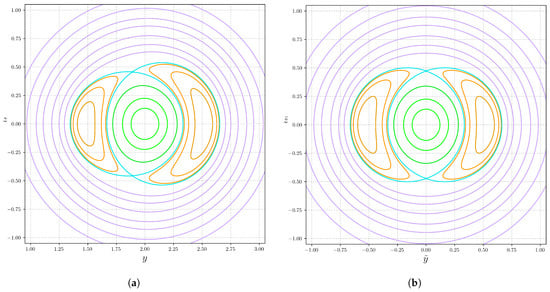
Figure 1. Level sets of $\mathrm{\Psi }$ on the poloidal section $\varphi =0$ for $(m,n)=(2,1)$ and standard values given by (16), in Cartesian (a) and symplectic (b) coordinates. The tori are coloured according to the region: inner (green), magnetic island (yellow), outer (magenta) and the separatrices (cyan).

3. Results

In this section, we apply the formulae in Equation (1) and Theorem 1 to the axisymmetric field (6), and the Equation (1) and Theorems 3’ and 4 to the field (12). As previously mentioned, the results in all forthcoming figures are presented over the poloidal plane $\varphi =0$.

For the computation of the volume Formula (1), we employ a regular grid in a convenient set of Cartesian coordinates $(\mathsf{x},\mathsf{y})$ over the chosen poloidal plane, in order to approximate the area element appearing in the volume formula. More precisely, for the volume enclosed between the flux surfaces ${\mathrm{\Psi }}_0$ and ${\mathrm{\Psi }}_1$ (with ${\mathrm{\Psi }}_1>{\mathrm{\Psi }}_0$), we consider

$$\mathcal{D}=\{({\mathsf{x}}_m,{\mathsf{y}}_n)\in {\mathbb{R}}^2:{\mathrm{\Psi }}_0<\mathrm{\Psi }({\mathsf{x}}_m,{\mathsf{y}}_n)<{\mathrm{\Psi }}_1\},$$

(18)

where $({\mathsf{x}}_m,{\mathsf{y}}_n)$ are the nodes of an $N_1\times N_2$ regular grid over the domain $[{\mathsf{x}}_0-L_1,{\mathsf{x}}_0+L_1]\times [{\mathsf{y}}_0-L_2,{\mathsf{y}}_0+L_2].$ If $\beta$ in these coordinates (restricted to the poloidal plane) takes the form

$${\beta }_P=f(\mathsf{x},\mathsf{y})d\mathsf{x}\wedge d\mathsf{y},$$

(19)

then the volume Formula (1) is approximated by

$$V\sim {\displaystyle \frac{4L_1{L}_2}{N_1{N}_2}}\sum _{i=1}^{N_1}\sum _{j=1}^{N_2}\mathsf{T}({\mathsf{x}}_i,{\mathsf{y}}_j)\left|f({\mathsf{x}}_i,{\mathsf{y}}_j)\right|·1_{\{({\mathsf{x}}_i,{\mathsf{y}}_j)\in \mathcal{D}\}}.$$

(20)

In the first example, the axisymmetric magnetic field, the convenient coordinates are $(R,z)$ over the poloidal plane $\varphi =0$. In this case, $\beta$ restricted to the poloidal section takes the form:

$${\beta }_P=-B^{\varphi }RdR\wedge dz=-{\displaystyle \frac{C}{R}}dR\wedge dz,$$

(21)

therefore, for this case: $|f(R_i,z_j)|=C/R_i$.

For the second example, we employ the symplectic coordinates $(\tilde{y},\tilde{z})$, since the areas are equivalent whether computed in $(\tilde{y},\tilde{z})$ or in $(\psi ,\vartheta )$, by  $d\tilde{y}\wedge d\tilde{z}=B_0^{-1}d\psi \wedge d\vartheta$. Thus, $\beta$ restricted to the poloidal section $\varphi =0$ can be written as,

$${\beta }_P=B^{\varphi }\sqrt{\left|g\right|}d\psi \wedge d\vartheta =B_{0}d\tilde{y}\wedge d\tilde{z};$$

(22)

therefore, for the second example: $|f({\tilde{y}}_i,{\tilde{z}}_j)|=|B_0|$.

Note, however, that the accuracy of (20) cannot be expected to be better than $O\left({\left(N_1{N}_2\right)}^{-3/4}\right)$; see for example, the classic cases of Gauss and Dirichlet for the number of grid points inside a circle or under a hyperbola [20]. Partly for this reason, and partly to see if we could improve the efficiency of computation of $V\left(\mathrm{\Psi }\right)$ as a function of $\mathrm{\Psi }$ (not just individual values of $\mathrm{\Psi }$), we also tested the method in the Appendix A. For this purpose, we established an algorithm to determine the level sets of $\mathrm{\Psi }(\tilde{y},\tilde{z},\varphi =0)={\mathrm{\Psi }}_0$ on the poloidal plane, which then is discretised into a regular partition of $N_g$ points $\left\{{\nu }_j\right\}$. With it, we computed (A1) by,

$${\displaystyle \frac{dV}{d\mathrm{\Psi }}}\left({\mathrm{\Psi }}_0\right)\sim \sum _{j=1}^{N_g}\mathsf{T}\left({\nu }_j\right)i_{{ϵ}_j}\lambda ,$$

(23)

where ${ϵ}_j$ denotes half displacement between ${\nu }_{j-1}$ and ${\nu }_{j+1}$, and $\lambda =i_B{i}_n\mathrm{\Omega }$, with $n=\nabla \mathrm{\Psi }/{|\nabla \mathrm{\Psi }|}^2$. To simplify the computations for the second example, we used the diagonal metric

$$d{s}^2={\displaystyle \frac{1}{2B_0\psi }}d{\psi }^2+{\displaystyle \frac{2\psi }{B_0}}d{\vartheta }^2+R_0^{2}d{\varphi }^2,$$

to compute $\nabla \mathrm{\Psi }$ and $i_{{ϵ}_j}\lambda =detW/B^{\varphi }$, where W is a matrix whose columns are the contravariant components of $(n,B,{\epsilon }_j)$ in the $(\psi ,\vartheta ,\varphi )$ coordinate system.

The implementation of (A1) for the first example used a discretisation ${\nu }_j$ of the level sets of $\mathrm{\Psi }$ with coordinates $R_j=(1+\sqrt{2\mathrm{\Psi }}cos{\theta }_j),z_j=\sqrt{2\mathrm{\Psi }}sin{\theta }_j$ and ${\theta }_j=2\pi /N$, $j=0,1,\dots ,N-1$. Following the steps in the Appendix A, (23) reduces in this case to

$${\displaystyle \frac{dV}{d\mathrm{\Psi }}}\left({\mathrm{\Psi }}_0\right)\sim C\sum _{j=0}^{N-1}{\displaystyle \frac{\mathsf{T}\left({\nu }_j\right)sin(2\pi /N)}{1+\sqrt{2\mathrm{\Psi }}cos{\theta }_j}}.$$

(24)

In contrast, for the integration of the volume formulae in Theorems 1, 3’ and 4, and the integration of (23), the trapezoidal rule was applied over a uniform grid in $\mathrm{\Psi }$, and the LSODA algorithm (Python’s scipy implementation) was employed for the field-line integration. All codes used an a priori short integration time for the fieldline (to get away from the initial line) and then extended it until the minimum number of crossings, $N_c$, required by the corresponding formula was attained.

Details about the codes used in the computations are provided in the Supplementary Materials.

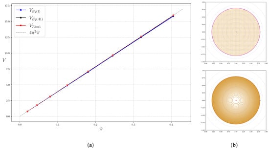
3.1. Axisymmetric Magnetic Field—Theorem 1

The left subplot in Figure 2 shows a comparison between the computations of the volume enclosed by the flux surfaces using the general Formula (1) and Theorem 1, for the axisymmetric magnetic field (1), as a function of the flux function $\mathrm{\Psi }$, defined in (7). The analytic volume given in (8) is also included. The volume formula (1) was computed over a regular array of points contained within a disc D of radius $\sqrt{2\mathrm{\Psi }}$, with $\mathrm{\Psi }$ taken from (7). For the volume computation using Theorem 1, only one initial point $x=(1+\sqrt{2\mathrm{\Psi }},0)$ was used to compute $T\left(\mathrm{\Psi }\right)$. The right inset in Figure 2 shows an example of the regular grid used to compute (8) and the flux surfaces corresponding to a uniform discretisation on $\mathrm{\Psi }$ used in Theorem 1.

Figure 2. (a) Volume enclosed by the flux-surface computed by (1) (blue), (A1) (black), Theorem 1 (red) and exact formula (8) (dashed grey) as a function of $\mathrm{\Psi }$ for the field (6), with $C=1$. (b) Example of the grid (top) and set of flux surfaces (bottom) used to compute (1) and Theorems 1, respectively.

3.2. Toroidal Helical Magnetic Field—Theorems 3’ and 4

The example considered corresponds to the magnetic field derived from (11) for one mode, namely the resonance $2/1$, that is

$$A_{\varphi }=-\left[\psi /4+{\psi }^2+\epsilon \psi (\psi -4)cos(2\vartheta -\varphi )\right].$$

(25)

Thus, (13) becomes $\mathrm{\Psi }=-\psi -2A_{\varphi }$, which implies that vector field u takes the form,

$$u={\partial }_{\vartheta }+2{\partial }_{\varphi }.$$

(26)

Write

$$v=B/\rho ,$$

(27)

with $\rho =B^{\varphi }$.

As the vector field u in (26) is constant with integer components (and thus commensurate), the u-lines are closed and all have period $2\pi$ in this case. Consequently, one of the lattice generators can be written as $T_1={(2\pi ,0)}^{\mathrm{T}}$ (superscript ^T denotes transpose, and flowing for time $2\pi$ along u and for 0 along v produces the identity map on any flux surface). The generator $T_2$ can be obtained through the return time T along v to any chosen u-line, using $T_2={(-c,T)}^{\mathrm{T}}$, where $-c$ is the time needed to flow along u to reach the initial point again. This is illustrated in Figure 3 for the tori in the inner and outer regions. Thus, the determinant in the volume formula for this case (Theorem 3’) takes the form

$$\mathrm{\Delta }\left(\mathrm{\Psi }\right)=2\pi T\left(\mathrm{\Psi }\right),$$

where $T\left(\mathrm{\Psi }\right)$ is the return time to the u-line along the scaled field v. The value of c is irrelevant for this. Thus, one factor in the volume formula for this example happens to take a similar form as in Theorem 1.

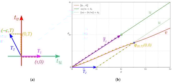
Figure 3. Selection of the lattice generators $T_1$ and $T_2$ for a torus in the inner region. (a): Generators $T_j$ in $(t_u,t_v)$-coordinates, corresponding to the flow times under the u- and v-fields. (b): Vectors ${\tilde{T}}_j$, the images of $T_j$ under ${\phi }_T(0,0)$ in the $(\varphi ,\vartheta )$-plane. ${\tilde{T}}_1$ (in purple) is drawn over an orbit of u (in green) through the initial point $(0,0)$; one translate of the u-orbit is also shown in green. The construction of ${\tilde{T}}_2$ requires the flow of T units under v (along the red curve) and then $-c$ units under u.

The other factor, namely $1/\widehat{\rho }$, is computed by averaging $1/\rho$ over a regular subdivision of the lattice $\mathrm{\Gamma }$, as described in Section 2.1.3. Figure 4 shows $1/\widehat{\rho }$ computed in the three regions for subdivisions by $q=4-12$. We see convergence for practical purposes when $q=6$, except near the separatrix. The convergence near the separatrix is less good, because analyticity of the AL coordinates fails in the separatrix limit, but the true value of $1/\widehat{\rho }$ is just the time-average of $1/\rho$ along the hyperbolic closed fieldline (≈1.94399). The approach of $1/\widehat{\rho }$ to the separatrix value is consistent with the form $\delta \mathrm{\Psi }log\delta \mathrm{\Psi }$, as is to be expected from the typical logarithmic divergence of return times near a hyperbolic periodic orbit. We use $q=6$ in our calculations of enclosed volume.

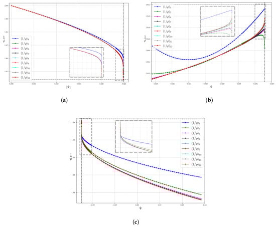
Figure 4. Average $1/\widehat{\rho }$ computed for subdivisions of sizes $q=4-12$: ${⟨1/\rho ⟩}_q$, as a function of $\mathrm{\Psi }$ in the three regions: (a) inner, (b) magnetic island, and (c) outer regions. The vertical lines indicate the value of $\mathrm{\Psi }$ for the separatrix, and the horizontal dash–dot line indicates the numerical value of $⟨1/\rho ⟩$ on the hyperbolic closed fieldline. Details of the plots near the separatrix are shown in dashed insets.

In the case of tori within a magnetic island, the visualisation on the $(\varphi ,\vartheta )$ plane is insufficient, as these coordinates are not well suited to describing an island torus. In these coordinates, the v-orbit appears to oscillate around the u-line, as shown in the right-hand inset of Figure 5. But the first apparent intersection of the v-orbit with the u-line is actually an illusion caused by a two-to-one projection of the flux surface to $(\varphi ,\vartheta )$. This apparent first crossing triggers the code to search for a second crossing ($N_c=2$, instead of 1 as in the two other regions).

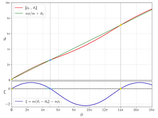
Figure 5. Plot in the $(\varphi ,\vartheta )$ plane of the orbit (red) and the u-line (green) starting at the point $(\tilde{y},\tilde{z})=(0.570,0.211)$ within the magnetic island. The first intersection in this plot, between the orbit and the u-line, does not correspond to an actual crossing, but rather to the orbit passing through a different point $({\psi }_1,{\vartheta }_1,{\varphi }_1)$ on the flux surface that satisfies ${\vartheta }_0={\vartheta }_1-n{\varphi }_1/m$ but not ${\psi }_1={\psi }_0$.

For Theorem 4, choosing $\gamma$ to be a u-line (i.e., $\psi$ = constant and $2\vartheta -\varphi$ = constant), we have that,

$$\begin{array}{c}\hfill \begin{array}{cc}\hfill \mathrm{\Phi }=& {\int }_{\gamma }{A}^{♭}={\int }_{\gamma }(A_{\psi }d\psi +A_{\vartheta }d\vartheta +A_{\varphi }d\varphi )\hfill \\ \hfill =& {\int }_{\gamma }\{\psi d\vartheta -\left[\psi /4+{\psi }^2+\epsilon \psi (\psi -4)cos(2\vartheta -\varphi )\right]d\varphi )\}\hfill \\ \hfill =& 2\pi \psi -4\pi [\psi /4+{\psi }^2+\epsilon \psi (\psi -4)cos(2{\vartheta }_0-{\varphi }_0)]\hfill \\ \hfill =& -2\pi \mathrm{\Psi }(\psi ,{\vartheta }_0,{\varphi }_0).\hfill \end{array}\end{array}$$

(28)

Therefore, the volume formula for this example again takes a form similar to that in Theorem 1: $dV=2\pi \overline{T}d\mathrm{\Psi },$ where the average $\overline{T}$ is computed using the unscaled magnetic field B. We found it to be sufficiently accurate when estimated by averaging the first ten crossings.

Figure 6 shows the averages of the return time, ${⟨T⟩}_N$, over the first N crossings as a function of $\mathrm{\Psi }$, with $N=1,10,20,30$, in the three regions: inner, island, and outer. The first plot uses $\left|\mathrm{\Psi }\right|$ on the x-axis (rather than $\mathrm{\Psi }$, which is negative there) to make it go from the magnetic axis on the left to the separatrix on the right. The value of $\mathrm{\Psi }$ corresponding to the separatrix is indicated by a vertical dashed line in all three subplots, coinciding with the divergence of T.

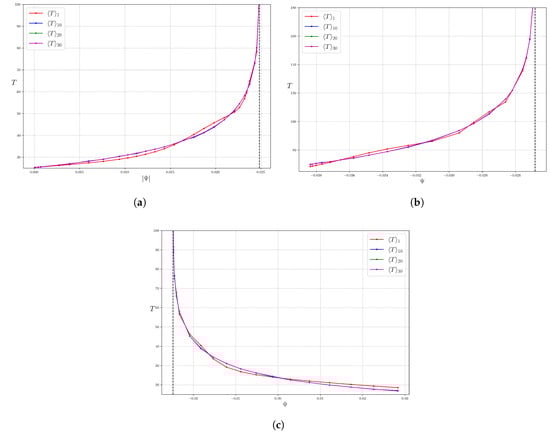
Figure 6. Averages of the return time ${⟨T⟩}_N$ of an unscaled field-line to a u-line as a function of $\mathrm{\Psi }$ in the three regions: inner (a), magnetic island (b) and outer (c) regions. The vertical lines indicate the value of $\mathrm{\Psi }$ for the separatrix.

In the next subsections, we give a little more detail about how we determine the lattice generators and give the results for the enclosed volumes for the three types of flux surface in this example.

3.2.1. Inner Region

For the inner region, a typical computation of $T_2\left(\mathrm{\Psi }\right)$ is displayed in Figure 7. From the theory, the return time along v to a given u-line is independent of the initial point on the u-line, but we checked this numerically and confirmed it. Also, the return time $T_2$ diverges like $-log\delta \mathrm{\Psi }$ as a separatrix is approached (compare the period of a pendulum), Figure 8.

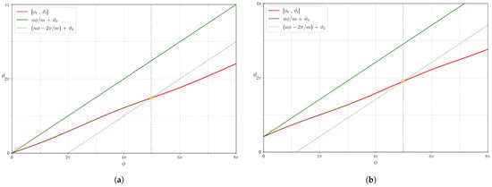
Figure 7. Crossing of the fieldline (red) and images of the u-line (green), starting at two selected initial points $({\tilde{y}}_i,{\tilde{z}}_i)$ on the poloidal plane $\varphi =0$: (a) $(0.2,0)$ and (b) $(0.06,0.21)$ on the same flux surface ($\mathrm{\Psi }=-0.01031$) in the inner region, for $\epsilon =0.007$. The return time along v is the same in both subplots $T\left(\mathrm{\Psi }\right)=15.60$.

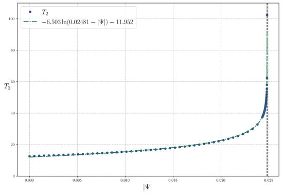
Figure 8. Return time $T_2$ along v, computed in the inner region (blue), and the fitted logarithmic curve $f\left(\mathrm{\Psi }\right)=-Aln(S-|\mathrm{\Psi }\left|\right)+B$ (green dash-dot line), with $S=0.0248157$ corresponding to the separatrix.

Figure 9 shows the volume computed by (1) and by Theorem 3 for the inner region as a function of $\mathrm{\Psi }$ defined in (13). We expected to see a more evident $\delta \mathrm{\Psi }log\delta \mathrm{\Psi }$ behaviour near the separatrix but it requires zooming in (not shown).

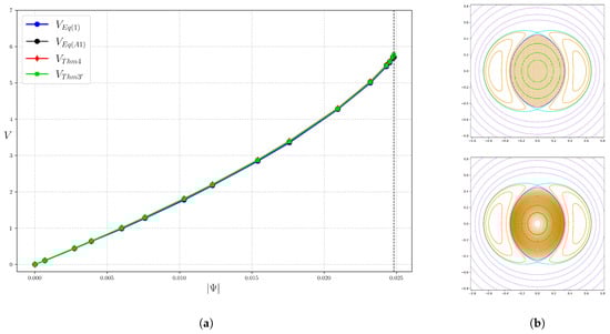
Figure 9. (a) Volume computed by (1) (blue), (A1) (black), Theorem 4 (red) and Theorem 3’ (green) as a function of $\left|\mathrm{\Psi }\right|$ (to make the slope positive) for the field (25) in the inner region. The vertical dashed line indicate the value of $\mathrm{\Psi }$ for the separatrix. (b) Example of the grid (top) and the set of flux surfaces (bottom), corresponding to a uniform partition in $\mathrm{\Psi }$, used to compute (1) and Theorems 3’ and 4, respectively.

3.2.2. Magnetic Island

A typical computation of $T_2\left(\mathrm{\Psi }\right)$ for the magnetic island region is displayed in Figure 10. As mentioned earlier in this section, $T_2$ is recorded for the second intersection between the fieldline and the u-line on the $(\varphi ,\vartheta )$-plane.

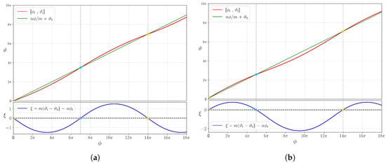
Figure 10. Crossing of the fieldline (red) and u-line (green) starting at two selected initial points $({\tilde{y}}_i,{\tilde{z}}_i)$ on the poloidal plane $\varphi =0$: $(0.4,0)$ and $(0.570,0.211)$ on the same flux surface ($\mathrm{\Psi }=-0.0316$) and same component, in the magnetic island region, for $\epsilon =0.007$. The second crossing time under v is the same in both subplots, $T\left(\mathrm{\Psi }\right)=43.86$, while the first (spurious crossing time) differs: 21.93 (a) and 15.53 (b). The blue graph in the bottom subplots corresponds to $\xi =m({\vartheta }_t-{\vartheta }_0)-n{\varphi }_t$, to more easily identify the crossings between the orbit and the u-line.

Figure 11 shows the volume computed by (1) and Theorem 3 for flux surfaces in the magnetic island as a function of $\mathrm{\Psi }$ defined in (13).

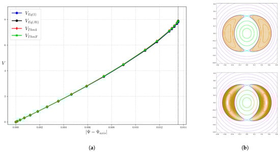
Figure 11. (a) Volume computed by (1) (blue), (A1) (black), Theorem 4 (red) and Theorem 3’ (green) as a function of $\mathrm{\Psi }$ for the field (25) in the magnetic island. The vertical dashed line indicate the value of $\mathrm{\Psi }$ for the separatrix. (b) Example of the grid (top) and the set of flux surfaces (bottom), corresponding to a uniform partition in $\mathrm{\Psi }$, used to compute (1), and Theorems 3’ and 4 and (A1), respectively.

3.2.3. Outer Region

A typical computation of $T_2\left(\mathrm{\Psi }\right)$ for the outer region is displayed in Figure 12.

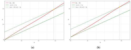
Figure 12. Crossing of the fieldline (red) and images of the u-line (green), starting at two selected initial points $({\tilde{y}}_i,{\tilde{z}}_i)$ on the poloidal plane $\varphi =0$: (a) $(0.7,0)$ and (b) $(0.41,0.54)$, on the same flux surface ($\mathrm{\Psi }=-0.01533$) in the outer region, for $\epsilon =0.007$. The return time is the same in both subplots $T\left(\mathrm{\Psi }\right)=18.15$.

Figure 13 shows the volume computed by (1) and Theorem 3 for the inner region as a function of $\mathrm{\Psi }$ defined in (13).

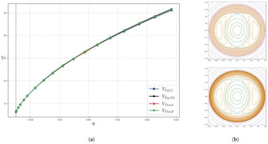
Figure 13. (a) Volume computed by (1) (blue), (A1) (black), Theorem 4 (red) and Theorem 3’ (green) as a function of $\mathrm{\Psi }$ for the field (25) in the outer region. The volumes enclosed by the island and inner regions has been added in. The vertical dashed line indicate the value of $\mathrm{\Psi }$ for the separatrix. (b) Example of the grid (top) and the set of flux surfaces (bottom), corresponding to a uniform partition in $\mathrm{\Psi }$, used to compute (1) and Theorems 3’ and 4, respectively.

4. Discussion

In this section, we discuss the performance of our implementations of the various methods of computation used in these examples. There are two aspects: computation time and accuracy of the result.

For the axisymmetric field, the volume computations of (1) and Theorem 1 were straightforward and the only parameter values to vary to improve the accuracy of the volume enclosed between a given ${\mathrm{\Psi }}_0$ and ${\mathrm{\Psi }}_1$, were the grid size for each method, as the integration times required to compute the respective return times are of the same order. In general, we found that Theorem 1 yields higher accuracy in only a fraction of the runtime of (1) or (A1), as illustrated in Table 1, which reports average runtimes for four values of $\mathrm{\Psi }$ from Figure 2, with grids chosen to achieve approximately 1% relative error for (1) and a coarse grid with $N=20$ for Theorem 1. Our implementation of (A1) was consistently faster and more accurate than (1), but not as efficient as Theorem 1. The average runtimes are given in seconds and correspond to single-core computations on an AMD^® Ryzen 5 3500U (2.1 GHz).

Table 1. Comparison of the volume estimation $V_0$, enclosed by the flux surfaces passing through $[1,0]$ (${\mathrm{\Psi }}_0=0$) and $[R_1,0]$ (${\mathrm{\Psi }}_1$), obtained using (1) and Theorem 1, with respect to grid size and average run time. The grid dimensions are $N_1\times N_2$ for (1), $N_g=N_2$ for the discretised level sets in (A1), and $N_{\mathrm{\Psi }}=N_1$ for integration in $\mathrm{\Psi }$ in (A1) and Theorems 3’ and 4. The rectangular domain for (1) is $[0.1,1.9]\times [-0.9,0.9]$.

${\mathit{R}}_1$	$\mathbf{\Psi }$	${\mathit{V}}_{\mathit{e}}$	Method	${\mathit{N}}_1$	${\mathit{N}}_2$	${\mathit{V}}_0$	$⟨{\mathit{t}}_0⟩$(s)	$\mathbf{\Delta }/{\mathbf{V}}_{\mathbf{e}}$
$1.2$	0.020	0.789568	Equation (1)	300	300	0.782214	67	0.009
			Equation (A1)	50	50	0.787261	56	0.003
			Theorem 1	20	—	0.789548	5	$2.6\times {10}^{-5}$
$1.4$	0.080	3.158273	Equation (1)	200	200	3.123140	107	0.011
			Equation (A1)	50	50	3.149079	57	0.003
			Theorem 1	20	—	3.158248	5	$7.9\times {10}^{-6}$
$1.6$	0.180	7.106115	Equation (1)	200	200	7.016993	240	0.012
			Equation (A1)	50	50	7.085340	57	0.003
			Theorem 1	20	—	7.106088	4	$3.8\times {10}^{-6}$
$1.8$	0.320	12.633094	Equation (1)	200	200	12.488658	403	0.011
			Equation (A1)	50	50	12.595751	58	0.003
			Theorem 1	20	—	12.633059	4	$2.7\times {10}^{-6}$

For the toroidal helical field, the computations of (1) and Theorems 3’ and 4 yielded comparable results but with significantly different runtimes. Accuracy was controlled by the grid sizes: $N\times N$ points in the poloidal section for (1), $N_g$ points to discretise a level set and N on $\mathrm{\Psi }$ for (A1), and N points in $\mathrm{\Psi }$ for Theorems 3’ and 4. We quantified accuracy by the relative error compared to a reference value $V^{*}$. The integration times for (1) and Theorem 3’ were of the same order, whereas that of Theorem 4 was required to be at least one order of magnitude greater to estimate the average return time. As (1) is equivalent to a three-dimensional integration, whereas (A1) and Theorems 3’ and 4 are equivalent to a bit more than two dimensions, one would expect the codes based on those theorems or (A1) to run faster than that for (1). In practice, however, for the small volumes between close flux surfaces ($|{\mathrm{\Psi }}_1-{\mathrm{\Psi }}_2|<ϵ$), our use of Theorem 4 can be slower than (1), and (A1) is the slowest of the four. There is a tradeoff between accuracy and computation time between our implementations of (1) and (A1), with the first being faster in small volumes and the second always more accurate, with a consistent computation time. Our implementation of (1) computes $\mathsf{T}$ only for the points in the grid contained between the level sets of ${\mathrm{\Psi }}_1$ and ${\mathrm{\Psi }}_2$, while that of (A1) computes $\mathsf{T}$ for every point in the discretised contour for N contours in the partition of $\mathrm{\Psi }$. Table 2 illustrates performance by reporting average runtimes for six $[{\mathrm{\Psi }}_1,{\mathrm{\Psi }}_2]$ intervals in the inner, island, and outer regions, using typical grid sizes. The reference values of ${\mathrm{\Psi }}_1$ correspond to the magnetic axis ($\mathrm{\Psi }=0$), the island O-point ($\mathrm{\Psi }=-0.0384$), and the separatrix ($\mathrm{\Psi }=-0.0248$). The reference volume $V_{*}$, used to compute the relative error, is obtained from Theorem 3’ with $N=400$, as this proved the most accurate and efficient method. More comparable implementations would allow more meaningful comparisons to be made.

Table 2. Comparison of the volume estimations $V_0$ enclosed by the flux surfaces ${\mathrm{\Psi }}_1$ and ${\mathrm{\Psi }}_2$, passing through $({\tilde{y}}_1,0)$ and $({\tilde{y}}_2,0)$, respectively. The estimates are obtained from (1), (A1) and Theorems 3’ and 4, with results shown against grid size, average runtime, and relative error with respect to a reference volume $V_{*}$. The grid dimensions are $N_1\times N_2$ for (1), $N_g=N_2$ for the discretised level sets in (A1), and $N_{\mathrm{\Psi }}=N_1$ for integration in $\mathrm{\Psi }$ in (A1) and Theorems 3’ and 4. The rectangular domains for (1) are inner region $[-0.335,0.335]\times [-0.47,0.47]$; island and outer regions $[-0.9,0.9]\times [-0.8,0.8]$. The reference volume $V_{*}$ is given by Theorem 3’ with $N=400$.

${\tilde{\mathit{y}}}_1$	${\mathbf{\Psi }}_1$	${\tilde{\mathit{y}}}_2$	${\mathbf{\Psi }}_2$	Region	Method	${\mathit{N}}_1$	${\mathit{N}}_2$	${\mathit{V}}_0$	$⟨{\mathit{t}}_0⟩$(s)	$\mathbf{\Delta }/{\mathit{V}}_{*}$
0	0.0	$0.150$	−0.0060	Inner	Equation (1)	300	300	0.997447	145	0.006
					Equation (A1)	100	100	1.002811	261	$7.7\times {10}^{-4}$
					Theorem 3’	100	—	1.013366	31	$9.7\times {10}^{-4}$
					Theorem 4	100	—	1.003619	115	$3.3\times {10}^{-5}$
0	0.0	$0.320$	−0.0245	Inner	Equation (1)	300	300	4.998763	652	0.005
					Equation (A1)	100	100	5.027210	252	$8.1\times {10}^{-4}$
					Theorem 3’	100	—	5.031270	30	0.002
					Theorem 4	100	—	5.031856	114	0.002
$0.52542$	−0.0384	$0.550$	−0.0380	Island	Equation (1)	500	500	0.155675	17	0.003
					Equation (A1)	100	100	0.154939	310	0.002
					Theorem 3’	100	—	0.155206	16	$5.1\times {10}^{-5}$
					Theorem 4	100	—	0.155038	58	0.001
$0.52542$	−0.0384	$0.662$	−0.0251	Island	Equation (1)	500	500	7.470030	640	0.005
					Equation (A1)	100	150	7.492240	623	0.002
					Theorem 3’	100	—	7.521046	18	0.002
					Theorem 4	100	—	7.519672	106	0.002
$0.66345$	−0.0248	$0.670$	−0.0240	Outer	Equation (1)	600	600	0.639184	58	0.014
					Equation (A1)	100	100	0.650239	361	0.003
					Theorem 3’	100	—	0.649799	44	0.002
					Theorem 4	100	—	0.650996	212	0.004
$0.66345$	−0.0248	$0.780$	0.0172	Outer	Equation (1)	600	600	7.736527	614	0.008
					Equation (A1)	100	100	7.906824	354	0.014
					Theorem 3’	100	—	7.904392	44	0.014
					Theorem 4	100	—	7.909134	173	0.014

In conclusion, our tests on Theorem 4 sometimes did not give efficient volume computations, but those on Theorem 3’ generally did. As most integrable cases can also be treated by Theorem 3’ after identification of a symmetry that conserves a density, our recommendation is to use Theorem 3’ (unless Theorems 2 or 1 apply, in which case the need to compute the harmonic average of the density is removed).

5. Conclusions

We computed the volumes enclosed by flux surfaces for two different integrable examples of magnetic fields using formulae provided by [2] and a new formula presented here for integrable fields with a symmetry field that preserves a density. The results of using different formulae are found to be consistent up to numerical error. As the methods are equivalent to 2D integration, they are mostly faster to compute than the standard 3D integration.

The volume estimation for the axisymmetric field between codes based on (1), (A1) and Theorem 1 confirmed that the latter was notably more efficient and accurate. This is evident in the comparison between a coarse grid in $\mathrm{\Psi }$ for Theorem 1 and a finer 2D grid for (1) and (A1) included in the previous section. Regarding the toroidal helical field, among the three formulae tested, the computational cost of Theorem 3’ was distinctly lower than that of (1) and Theorem 4, and exhibited faster numerical convergence. The accuracy of the integration in (1) was constrained by the resolution of the regular grid employed for its evaluation. Nevertheless, for flux surfaces with a small cross-section, (1) is more efficient than Theorem 4, since accurate integration along the flow lines was substantially more demanding, with lengths greater by approximately an order of magnitude (i.e., by a factor of ten).

A disadvantage of these methods is that they cannot be used to measure volumes enclosed by flux surfaces in fields that contain chaotic regions. It would be good to obtain an efficient formula for the flux enclosed by a flux surface of a general magnetic field. We plan to achieve and test this via a vector potential on the flux surface, which easily gives efficient formulae for enclosed toroidal and poloidal flux, and we have just worked out how to get it to give volume.

It would be desirable to test the formulae on numerically computed quasisymmetric fields as in [7]. The methods should also apply to approximately integrable fields with knotted or linked tori, as in Ref. [21], though it is difficult to make exactly integrable examples (indeed, we have conjectured many years ago that non-degenerate integrable vacuum fields have to be axisymmetric).

References

- Landreman, M.; Medasani, B.; Wechsung, F.; Giuliani, A.; Jorge, R.; Zhu, C. SIMSOPT: A flexible framework for stellarator optimization. J. Open Source Softw. 2021, 6, 3525. [Google Scholar] [CrossRef]
- MacKay, R.S. Volume enclosed by a flux surface. Proc. Steklov Inst. Math. 2024, 327, 226–235. [Google Scholar] [CrossRef]
- Helander, P. Theory of plasma confinement in non-axisymmetric magnetic fields. Rep. Prog. Phys. 2014, 77, 087001. [Google Scholar] [CrossRef] [PubMed]
- Huang, Y.M.; Hew, J.K.J.; Brown, A.; Bhattacharjee, A. Computation of magnetohydrodynamic equilibria with Voigt regularization. Phys. Plasmas 2025, 32, 062507. [Google Scholar] [CrossRef]
- MacKay, R.S. Differential forms for plasma physics. J. Plasma Phys. 2020, 86, 925860101. [Google Scholar] [CrossRef]
- Burby, J.; Kallinikos, N.; MacKay, R.S. Some mathematics for quasi-symmetry. J. Math. Phys. 2020, 61, 093503. [Google Scholar] [CrossRef]
- Landreman, M.; Paul, E. Magnetic fields with precise quasisymmetry for plasma confinement. Phys. Rev. Lett. 2022, 128, 035001. [Google Scholar] [CrossRef] [PubMed]
- Rodriguez, E.; Helander, P.; Bhattacharjee, A. Necessary and sufficient conditions for quasisymmetry. Phys. Plasmas 2020, 27, 062501. [Google Scholar] [CrossRef]
- Hamada, S. Hydromagnetic equilibria and their proper coordinates. Nuclear Fusion 1962, 2, 23. [Google Scholar] [CrossRef]
- Kallinikos, N.; MacKay, R.S.; Martinez-del Rio, D. Regions without flux surfaces of given class for magnetic fields in toroidal geometry. Plasma Phys. Control Fusion 2023, 65, 095021. [Google Scholar] [CrossRef]
- Arnol’d, V.I. Mathematical Methods of Classical Mechanics; Springer: Berlin/Heidelberg, Germany, 2013; Volume 60. [Google Scholar] [CrossRef]
- Weideman, J. Numerical integration of periodic functions: A few examples. Amer. Math. Monthly 2002, 109, 21–36. [Google Scholar] [CrossRef]
- Newcomb, W. Magnetic differential equations. Phys. Fluids 1959, 2, 362–365. [Google Scholar] [CrossRef]
- Perrella, D.; Duignan, N.; Pfefferlé, D. Existence of global symmetries of divergence-free fields with first integrals. J. Math. Phys. 2023, 64, 052705. [Google Scholar] [CrossRef]
- Perrella, D.; Pfefferlé, D.; Stoyanov, L. Rectifiability of divergence-free fields along invariant 2-tori. Partial Differ. Equ. Appl. 2022, 3, 50. [Google Scholar] [CrossRef]
- Burby, J.; MacKay, R.; Naik, S. Isodrastic magnetic fields for suppressing transitions in guiding-centre motion. Nonlinearity 2023, 36, 5884. [Google Scholar] [CrossRef]
- Martinez-del Rio, D.; MacKay, R.S. Conefield approach to identifying regions without flux surfaces for magnetic fields. Plasma Phys. Control. Fusion 2025, 67, 055005. [Google Scholar] [CrossRef]
- Kallinikos, N.; Isliker, H.; Vlahos, L.; Meletlidou, E. Integrable perturbed magnetic fields in toroidal geometry: An exact analytical flux surface label for large aspect ratio. Phys. Plasmas 2014, 21, 064504. [Google Scholar] [CrossRef]
- Abdullaev, S. Magnetic Stochasticity in Magnetically Confined Fusion Plasmas; Springer: Berlin/Heidelberg, Germany, 2014; p. 412. [Google Scholar] [CrossRef]
- Huxley, M. Area, Lattice Points, and Exponential Sums; Clarendon Press: Oxford, UK, 1996; Volume 13. [Google Scholar] [CrossRef]
- Hudson, S.; Startsev, E.; Feibush, E. A new class of magnetic confinement device in the shape of a knot. Phys. Plasmas 2014, 21, 010705. [Google Scholar] [CrossRef]
Disclaimer/Publisher’s Note: The statements, opinions and data contained in all publications are solely those of the individual author(s) and contributor(s) and not of MDPI and/or the editor(s). MDPI and/or the editor(s) disclaim responsibility for any injury to people or property resulting from any ideas, methods, instructions or products referred to in the content. |
© 2025 by the authors. Licensee MDPI, Basel, Switzerland. This article is an open access article distributed under the terms and conditions of the Creative Commons Attribution (CC BY) license (https://creativecommons.org/licenses/by/4.0/).