On Bregman Asymptotically Quasi-Nonexpansive Mappings and Generalized Variational-like Systems

Abstract

In this work, we propose and study an inertial hybrid projection algorithm to approximate a common solution of a system of unrelated generalized mixed variational-like inequalities and the common fixed points of Bregman asymptotically quasi-nonexpansive mappings in the intermediate sense. We establish a strong convergence theorem for the generated sequence and derive several corollaries. Further, we provide applications of Bregman asymptotically quasi-nonexpansive mappings in the intermediate sense. Numerical examples are provided to demonstrate the effectiveness of the method, and we also present a comparative analysis.

1. Introduction

Let E denote a real Banach space with dual space $E^{*}$, equipped with the duality pairing $⟨·,·⟩$. Let Q be a nonempty, closed, and convex subset of E. We investigate a system of unrelated generalized mixed variational-like inequality problems (SUGMVLIPs). For an index set $\Delta$, suppose that, for every $i\in \Delta$, $Q_i$ is a nonempty closed convex subset of E satisfying ${\bigcap }_{i\in \Delta }{Q}_i\ne \varnothing$. Further, let ${\mathcal{H}}_i:Q_i\times Q_i\times Q_i\to \mathbb{R}$ and ${\mathfrak{f}}_i:Q_i\times Q_i\to \mathbb{R}$ be given nonlinear mappings. The SUGMVLIP is to find a point $w\in \mathcal{Q}={\bigcap }_{i\in \Delta }{Q}_i$ such that

$${\mathcal{H}}_i(y_i,w;w)+{\mathfrak{f}}_i(w,y_i)-{\mathfrak{f}}_i(w,w)\ge 0,\forall y_i\in Q_i.$$

(1)

Let $\mathsf{\Omega }={\bigcap }_{i\in \Delta }{\Gamma }_i$ be the solution set of SUGMVLIP (1), where ${\Gamma }_i$ is the solution set for the GMVLIP defined by ${\mathcal{H}}_i$, ${\mathfrak{f}}_i$, and $Q_i$.

In the case where E is a Hilbert space H endowed with the inner product $⟨·,·⟩$, if we set ${\mathfrak{f}}_i=0$ and define ${\mathcal{H}}_i(y_i,w;w)={\mathcal{G}}_i(w,y_i)+⟨{\mathcal{A}}_{i}w,y_i-w⟩$ for mappings ${\mathcal{G}}_i:Q_i\times Q_i\to \mathbb{R}$ and ${\mathcal{A}}_i:H\to H$, then SUGMVLIP (1) simplifies to the system of unrelated mixed equilibrium problems examined by Djafari-Rouhani et al. [1].

In the particular case where ${\mathcal{H}}_i=0$ and ${\mathfrak{f}}_i=0$ for every index i, the SUGMVLIP (1) reduces to the convex feasibility problem (CFP), which involves locating a point $w\in {\bigcap }_{i\in \Delta }{Q}_i$. Moreover, when each set $Q_i$ coincides with the fixed-point set of a corresponding operator ${\mathcal{S}}_i:E\to E$, the CFP is equivalent to the common fixed-point problem (CFPP).

When the index set contains a single element (i.e., $i=1$), SUGMVLIP (1) becomes equivalent to the following GMVLIP: find an element $w\in Q$ satisfying

$$\mathcal{H}(y,w;w)+\mathfrak{f}(w,y)-\mathfrak{f}(w,w)\ge 0,\forall y\in Q.$$

(2)

This formulation was initially proposed by Kazmi et al. [2] and was subsequently analyzed in [3].

By taking $\mathfrak{f}=0$ in inequality (2), we obtain the general variational-like inequality problem (GVLIP), which requires finding a point $w\in Q$ that satisfies

$$\mathcal{H}(y,w;w)\ge 0,\forall y\in Q.$$

(3)

This problem was first formulated by Preda et al. [4] and later investigated by Mahato and Nahak [5].

Consider the specialization where $\mathcal{H}(y,w;w)=⟨\mathcal{B}w,\eta (y,w)⟩$, with mappings $\mathcal{B}:Q\to E^{*}$ and $\eta :Q\times Q\to E$, and where $\mathfrak{f}=0$. This case corresponds to the variational-like inequality problem (VLIP): find $w\in Q$ such that

$$⟨\mathcal{B}w,\eta (y,w)⟩\ge 0,\forall y\in Q.$$

Parida et al. [6] originally introduced this problem, which finds important applications in mathematical programming.

In the specific case where $\eta (y,w)=y-w$, the variational-like inequality problem simplifies to the classical variational inequality problem (VIP): determine an element $w\in Q$ for which

$$⟨\mathcal{B}w,y-w⟩\ge 0,\forall y\in Q.$$

(4)

This formulation was initially examined by Hartmann and Stampacchia [7].

If we set $\mathfrak{f}=0$; $E={\mathbb{R}}^n$; $\mathcal{H}(y,w;w)=⟨▽\mathcal{B}w,\eta (y,w)⟩$, where $\eta :Q\times Q\to {\mathbb{R}}^n$ is continuous and $\mathcal{B}:Q\to {\mathbb{R}}^n$ is differentiable and $\eta$-convex [6], then GMVLIP (2) is reduced to the following mathematical programming problem:

$$\underset{w\in Q}{min}\mathcal{B}\left(w\right).$$

As a final special case, setting $\mathcal{H}(y,w;w)=\mathcal{G}(w,y)$ and $\mathfrak{f}\equiv 0$ transforms GMVLIP (2) into the equilibrium problem (EP): find a point $w\in Q$ satisfying

$$\mathcal{G}(w,y)\ge 0,\forall y\in Q.$$

(5)

This problem was first presented by Blum and Oettli [8]. We denote the solution set of EP (5) by $\mathrm{Sol}\left(\mathrm{EP}\right)$.

The generalized mixed variational-like inequality problem (GMVLIP) is known to be a trifunction equilibrium problem, with the classical equilibrium problem as its special case. This framework has significantly influenced various fields of science and engineering, unifying several theories in nonlinear analysis, optimization, economics, finance, game theory, physics, and engineering. Moreover, both GMVLIP and the equilibrium problem encompass many well-known problems as particular cases, including mathematical programming, variational inequalities and inclusions, complementarity, saddle point, Nash equilibrium, minimax, minimization, and fixed-point problems; see [3,8,9,10].

Recall that a mapping $\mathcal{T}$ is said to be nonexpansive if

$$\parallel \mathcal{T}p-\mathcal{T}u\parallel \le \parallel p-u\parallel ,\forall p,u\in Q$$

More generally, $\mathcal{T}$ is said to be asymptotically nonexpansive if there exists a sequence $\left\{{\xi }_n\right\}$ with $\underset{n\to \infty }{lim}{\xi }_n=1$ such that

$$\parallel {\mathcal{T}}^{n}p-{\mathcal{T}}^{n}u\parallel \le {\xi }_n\parallel p-u\parallel ,\forall p,u\in Qandn\ge 1.$$

In Hilbert spaces, Takahashi et al. [11] proposed a hybrid iterative algorithm using projection methods for nonexpansive mappings, ensuring strong convergence without compactness assumptions. Schu [12] introduced a modified Mann iteration for asymptotically nonexpansive mappings in uniformly convex Banach spaces. Motivated by these works, Inchan [13] developed a hybrid projection algorithm incorporating the modified Mann iteration for asymptotically nonexpansive mappings. The mapping $\mathcal{T}$ is said to be asymptotically nonexpansive in the intermediate sense if

$$\underset{n\to \infty }{lim}sup\underset{p,u\in Q}{sup}(\parallel {\mathcal{T}}^{n}p-{\mathcal{T}}^{n}u\parallel -\parallel p-u\parallel )\le 0.$$

(6)

If $F\left(\mathcal{T}\right)\ne \varnothing$ and (6) holds for all $p\in Q$ and $u\in F\left(\mathcal{T}\right)$, then $\mathcal{T}$ is said to be asymptotically quasi-nonexpansive in the intermediate sense.

Remark 1.

It is worth noting that asymptotically quasi-nonexpansive mappings in the intermediate sense form a broader class than asymptotically nonexpansive mappings since the mappings in the intermediate sense are not necessarily Lipschitz continuous.

Qin et al. [14] introduced an iterative scheme in 2009 for addressing an EP alongside the fixed points of two $\varphi$-nonexpansive mappings within a uniformly convex and uniformly smooth Banach space. Their algorithm is defined by the following steps:

$$\left.\begin{array}{c}{w}^0\in Q,Q^0=Q,\hfill \\ z^n=J^{-1}({\alpha }^{n}J{w}^n+{\beta }^{n}J\mathcal{S}{w}^n+{\gamma }^{n}J\mathcal{T}{w}^n),\hfill \\ q^n=T_{r^n}{z}^n,\hfill \\ Q^{n+1}=\{p\in Q^n:\varphi (p,q^n)\le \varphi (p,w^n)\},\hfill \\ w^{n+1}={\mathsf{\Pi }}_{Q^{n+1}}{w}^0,\hfill \end{array}\right\}$$

(7)

Here, ${\mathsf{\Pi }}_Q$ denotes the generalized projection, the Lyapunov functional is given by $\varphi (w,y)={\parallel w\parallel }^2-2⟨y,Jw⟩+{\parallel y\parallel }^2$, and J represents the normalized duality mapping with inverse $J^{-1}$. By using hybrid projection method, Kazmi et al. [15] proved a strong convergence theorem for an asymptotically quasi-$\varphi$-nonexpansive with respect to Lyapunov function in the intermediate sense and solution of EP (5). More generalization can be found in [3,16,17].

In 1967, Bregman [18] introduced a significant technique based on the concept of the Bregman distance function. This approach has proven to be highly effective not only in the design and analysis of iterative methods but also in addressing a wide range of problems, including optimization, feasibility, equilibrium approximation, fixed-point computations, and variational inequalities (see [19,20]). In 2010, Reich et al. [21] proposed an iterative algorithm in Banach spaces involving maximal monotone operators. Building on the framework of Bregman projections, numerous iterative algorithms have since been developed and analyzed by researchers in this area (see, for example, [19,22,23,24,25,26]).

Several researchers have investigated iterative methods for approximating fixed points of nonexpansive mappings using the Bregman distance (see, for example, [24,27]). However, only a few have considered nonlinear mappings that are not Lipschitz continuous (see, for example, [28,29]).

Maingé [30] introduced the inertial Krasnosel’skiĭ–Mann iteration in 2008:

$$\left.\begin{array}{c}{t}^n=w^n+{\theta }_n(w^n-w^{n-1}),\hfill \\ w^{n+1}=(1-{\alpha }^n)t^n+{\alpha }^{n}T{t}^n,\hfill \end{array}\right\}$$

(8)

proving weak convergence. Bot et al. [31] later relaxed some assumptions in Maingé’s analysis. Further developments can be found in [3,32,33,34]. The efficiency of inertial methods has been demonstrated in various applications, including imaging and data analysis [35,36,37].

It is noteworthy that convergence analysis of inertial iterative methods in Banach spaces remains largely unexplored. Therefore, the purpose of this paper is to introduce an inertial projection iterative algorithm and prove a strong convergence theorem to approximate the common solution of SUGMVLIP (1) and asymptotically quasi-nonexpansive mappings with respect to Bregman distance in the intermediate sense without considering the Lipschitz continuous assumption of the mapping. Building upon the foundational research in [2,15,24,28,29,30], this paper presents a novel inertial hybrid iterative algorithm that incorporates Bregman asymptotically quasi-nonexpansive mappings in the intermediate sense. Our main contributions include establishing a strong convergence theorem for the generated iterative sequences, deriving important corollaries that extend the applicability of our results, and demonstrating the practical utility of the approach through numerical experiments that highlight its efficiency and relevance. Also, we provide the MATLAB-Style Pseudocode of our main algorithm in Appendix A.

2. Preliminaries

Let symbols → and ⇀ denote strong and weak convergence, respectively. Throughout the rest of the paper, unless specified, let E be a reflexive Banach space. Let $\mathrm{dom}h=\{u\in E:h(u)<+\infty \}$ denote the effective domain of h. Consider a proper, convex, and lower semicontinuous function $h:E\to (-\infty ,+\infty ]$, and let $h^{*}:E^{*}\to (-\infty ,+\infty ]$ be its Fenchel conjugate, defined by

$$h^{*}\left(w_0\right)=sup\left\{⟨w_0,p⟩-h\left(p\right):p\in E\right\},w_0\in E^{*}.$$

Moreover, for any $p\in \mathrm{int}\left(\mathrm{dom}h\right)$ and $u\in E$, the right-hand directional derivative of h at p in the direction u is given by

$$h^0(p,u)=\underset{\mu \to 0^{+}}{lim}{\displaystyle \frac{h(p+\mu u)-h\left(p\right)}{\mu }}.$$

The function h is said to be Gâteaux differentiable at p if the limit defining $h^0(p,u)$ exists for all directions u. In this case, $h^0(p,u)$ coincides with $⟨\nabla h\left(p\right),u⟩$, where $\nabla h\left(p\right)$ denotes the gradient of h at p. The function h is said to be Fréchet differentiable at p if this limit is attained uniformly in $\parallel u\parallel =1$. Finally, h is said to be uniformly Fréchet differentiable on a subset Q of E if the above limit is attained uniformly for $p\in Q$ and $\parallel u\parallel =1.$

The Legendre function h is defined from a general Banach space E into $(-\infty ,+\infty ];$ see [19]. Since E is reflexive, according to [19], the function h is Legendre if it satisfies the following conditions:

(L1)

The interior of its domain is nonempty ($int(domh)\ne \varnothing$), h is Gâteaux differentiable on $int(domh)$, and $dom\nabla h=int(domh)$;

(L2)

The interior of the domain of its conjugate is nonempty ($int(dom{h}^{*})\ne \varnothing$), $h^{*}$ is Gâteaux differentiable on $int(dom{h}^{*})$, and $dom\nabla h^{*}=int(dom{h}^{*})$.

The following properties hold for Legendre functions [19]:

(P1)

h is Legendre if and only if $h^{*}$ is Legendre;

(P2)

The subdifferential inverse satisfies ${(\partial h)}^{-1}=\partial h^{*}$;

(P3)

The gradients are inverses: $\nabla h={(\nabla h^{*})}^{-1}$, with $ran\nabla h=dom\nabla h^{*}=int(dom{h}^{*})$ and $ran\nabla h^{*}=dom\nabla h=int(domh)$;

(P4)

Both h and $h^{*}$ are strictly convex on $int(domh)$ and $int(dom{h}^{*})$, respectively.

Example 1.

The following examples of Legendre function were presented in [19]:

(1)

Suppose $1<p<+\infty$ and $h\left(x\right)={\displaystyle \frac{1}{p}}{\left|x\right|}^p$ on $int(domh)=\mathbb{R}.$ Then, $h^{*}\left(x^{*}\right)={\displaystyle \frac{1}{q}}{\left|x^{*}\right|}^q$ on $int(dom{h}^{*})=\mathbb{R},$ where ${\displaystyle \frac{1}{p}}+{\displaystyle \frac{1}{q}}=1$. Hence, h and $h^{*}$ are Legendre.

(2)

Halved energy: $h\left(x\right)={\displaystyle \frac{1}{2}}{\parallel x\parallel }^2={\displaystyle \frac{1}{2}}{\sum }_{i=1}^n{x}_i^2$ is Legendre on $\mathbb{R}.$

(3)

Suppose $0<p<1$ and $h\left(x\right)=-{\displaystyle \frac{1}{p}}{x}^p$ on $int(domh)=[0,+\infty )$. Then, $h^{*}\left(x^{*}\right)=-{\displaystyle \frac{1}{q}}{(-x^{*})}^q$ on $int(dom{h}^{*})=(-\infty ,0),$ where ${\displaystyle \frac{1}{p}}+{\displaystyle \frac{1}{q}}=1$. Hence, h is Legendre, whereas $h^{*}$ is not.

(4)

De Pierro and Iusem: Suppose

$$h\left(x\right)=\left\{\begin{array}{cc}{\displaystyle \frac{1}{2}}(x^2-4x+3),\hfill & x\le 1,\hfill \\ -lnx,\hfill & otherwise,\hfill \end{array}\right.$$

on $int(domh)=\mathbb{R}$. Then,

$$h^{*}\left(x^{*}\right)=\left\{\begin{array}{cc}{\displaystyle \frac{1}{2}}{\left(x^{*}\right)}^2+2x^{*}+{\displaystyle \frac{1}{2}},\hfill & x^{*}\le -1,\hfill \\ -1-ln(-x^{*}),\hfill & -1\le x^{*}<0.\hfill \end{array}\right.$$

on $int(dom{h}^{*})=(-\infty ,0)$. Hence, h and $h^{*}$ are Legendre.

Definition 1

([18]). Let $h:E\to (-\infty ,+\infty ]$ be a convex function that is Gâteaux differentiable. The Bregman distance with respect to h is the function ${\mathcal{D}}_h:domh\times \mathit{int}(\mathit{dom}h)\to [0,+\infty )$ defined by

$${\mathcal{D}}_h(u,p)=h\left(u\right)-h\left(p\right)-⟨\nabla h\left(p\right),u-p⟩,$$

(9)

for $p\in \mathit{int}(\mathit{dom}h)$ and $u\in \mathit{dom}h$.

It is important to emphasize that the Bregman distance does not constitute a metric in the conventional sense. While ${\mathcal{D}}_h(p,p)=0$ is evident, the converse—that ${\mathcal{D}}_h(p,u)=0$ implies $p=u$—does not generally hold. However, this implication is valid when h is a Legendre function. Typically, ${\mathcal{D}}_h$ lacks symmetry and fails to satisfy the triangle inequality. Nevertheless, from its definition, several key identities follow [27]: for any $u,u_1,u_2\in \mathrm{dom}h$ and $s,p\in \mathrm{int}(\mathrm{dom}h)$,

(B1)

Two-point identity:

$${\mathcal{D}}_h(s,p)+{\mathcal{D}}_h(p,s)=⟨\nabla h\left(s\right)-\nabla h\left(p\right),s-p⟩;$$

(B2)

Three-point identity:

$${\mathcal{D}}_h(u,s)+{\mathcal{D}}_h(s,p)-{\mathcal{D}}_h(u,p)=⟨\nabla h\left(p\right)-\nabla h\left(s\right),u-s⟩;$$

(B3)

Four-point identity:

$${\mathcal{D}}_h(u_1,s)-{\mathcal{D}}_h(u_1,p)-{\mathcal{D}}_h(u_2,s)+{\mathcal{D}}_h(u_2,p)=⟨\nabla h\left(p\right)-\nabla h\left(s\right),u_1-u_2⟩.$$

Definition 2

([21,23]). Let $\mathcal{T}:Q\to \mathit{int}(\mathit{dom}g)$ be a mapping with fixed-point set $F\left(\mathcal{T}\right)=\{u\in Q:\mathcal{T}u=u\}$. The following definitions are employed:

(D1)

A point $u_0\in Q$ is an asymptotic fixed point of $\mathcal{T}$ if there exists a sequence $\left\{u_n\right\}\subset Q$ such that $u_n\rightharpoonup u_0$ and ${lim}_{n\to \infty }\parallel \mathcal{T}{u}_n-u_n\parallel =0$. The set of all asymptotic fixed points is denoted by $\widehat{F}\left(\mathcal{T}\right)$.

(D2)

The mapping $\mathcal{T}$ is Bregman quasi-nonexpansive (BQNE) if $F\left(\mathcal{T}\right)\ne \varnothing$ and

$${\mathcal{D}}_h(u_0,\mathcal{T}u)\le {\mathcal{D}}_h(u_0,u),\forall u\in Q,u_0\in F\left(\mathcal{T}\right).$$

(D3)

The mapping $\mathcal{T}$ is Bregman asymptotically quasi-nonexpansive in the intermediate sense (BAQNE) if $F\left(\mathcal{T}\right)\ne \varnothing$ and [28]

$$\underset{n\to \infty }{lim\; sup}\underset{\begin{array}{c}{u}_0\in F\left(\mathcal{T}\right)\\ u\in Q\end{array}}{sup}\left({\mathcal{D}}_h(u_0,{\mathcal{T}}^{n}u)-{\mathcal{D}}_h(u_0,u)\right)\le 0.$$

(10)

Defining ${\xi }_n=max\left\{0,\underset{\begin{array}{c}{u}_0\in F\left(\mathcal{T}\right)\\ u\in Q\end{array}}{sup}\left({\mathcal{D}}_h(u_0,{\mathcal{T}}^{n}u)-{\mathcal{D}}_h(u_0,u)\right)\right\}$, it follows that ${lim}_{n\to \infty }{\xi }_n=0$. Thus, inequality (10) is equivalent to

$${\mathcal{D}}_h(u_0,{\mathcal{T}}^{n}u)\le {\mathcal{D}}_h(u_0,u)+{\xi }_n,\forall u\in Q,u_0\in F\left(\mathcal{T}\right).$$

(D4)

The mapping $\mathcal{T}$ is Bregman relatively nonexpansive (BRNE) if $\widehat{F}\left(\mathcal{T}\right)=F\left(\mathcal{T}\right)\ne \varnothing$ and

$${\mathcal{D}}_h(u_0,\mathcal{T}u)\le {\mathcal{D}}_h(u_0,u),\forall u\in Q,u_0\in F\left(\mathcal{T}\right).$$

(D5)

The mapping $\mathcal{T}$ is Bregman firmly nonexpansive (BFNE) if, for all $u_1,u_2\in Q$,

$$⟨\nabla h\left(\mathcal{T}{u}_1\right)-\nabla h\left(\mathcal{T}{u}_2\right),\mathcal{T}{u}_1-\mathcal{T}{u}_2⟩\le ⟨\nabla h\left(u_1\right)-\nabla h\left(u_2\right),\mathcal{T}{u}_1-\mathcal{T}{u}_2⟩,$$

or, equivalently,

$${\mathcal{D}}_h(\mathcal{T}{u}_1,\mathcal{T}{u}_2)+{\mathcal{D}}_h(\mathcal{T}{u}_2,\mathcal{T}{u}_1)+{\mathcal{D}}_h(\mathcal{T}{u}_1,u_1)+{\mathcal{D}}_h(\mathcal{T}{u}_2,u_2)\le {\mathcal{D}}_h(\mathcal{T}{u}_1,u_2)+{\mathcal{D}}_h(\mathcal{T}{u}_2,u_1).$$

(D6)

The mapping $\mathcal{T}$ is asymptotically regular on Q if, for every bounded subset $C\subset Q$,

$$\underset{n\to \infty }{lim}\underset{u\in C}{sup}∥{\mathcal{T}}^{n+1}u-{\mathcal{T}}^{n}u∥=0.$$

Remark 2.

Note that Bregman asymptotically quasi-nonexpansive in the intermediate sense is not Lipschitz continuous in general.

Example 2.

Let $E=\mathbb{R}$, $Q=[{\displaystyle \frac{1}{2}},{\displaystyle \frac{3}{2}}]$, and $\mathcal{T}:Q\to Q$ be defined by

$$\mathcal{T}\left(u\right)=\left\{\begin{array}{cc}1,\hfill & u\in [{\displaystyle \frac{1}{2}},1],\hfill \\ 1-\sqrt{{\displaystyle \frac{u-1}{2}}},\hfill & u\in (1,{\displaystyle \frac{3}{2}}].\hfill \end{array}\right.$$

Note that $F\left(\mathcal{T}\right)=\left\{1\right\}$ and ${\mathcal{T}}^{n}u=1,\forall u\in Qandn\ge 2.$ If $h:\mathbb{R}\to (-\infty ,\infty )$ is a Legendre function, then $\mathcal{T}$ is a Bregman asymptotically quasi-nonexpansive in the intermediate sense since

$$\underset{n\to \infty }{lim\; sup}\underset{\begin{array}{c}u\in Q\end{array}}{sup}\left({\mathcal{D}}_h(1,{\mathcal{T}}^{n}u)-{\mathcal{D}}_h(1,u)\right)\le \underset{n\to \infty }{lim\; sup}\underset{\begin{array}{c}u\in Q\end{array}}{sup}{\mathcal{D}}_h(1,{\mathcal{T}}^{n}u)=0.$$

However, $\mathcal{T}$ is not Lipschitizian with respect to Bregman distance. Indeed, suppose that there exists $L>0$ such that ${\mathcal{D}}_h(\mathcal{T}p,\mathcal{T}u)\le L{\mathcal{D}}_h(p,u),\forall u,p\in Q.$ By Taylor’s theorem, there exists $t\in (0,1)$ such that

$${\mathcal{D}}_h(p,u)=h\left(p\right)-h\left(u\right)-⟨\nabla h\left(u\right),p-u⟩={\displaystyle \frac{1}{2}}{\nabla }^{2}h(u+t(p-u)){(p-u)}^2.$$

Let $h\left(u\right)={\displaystyle \frac{1}{2}}{\parallel u\parallel }^2$ on $int(domh)=\mathbb{R}$ and ${\mathcal{D}}_h(p,u)={\displaystyle \frac{1}{2}}{\parallel p-u\parallel }^2,\forall u,p\in \mathbb{R}$. Put $p=1$ and $u=1+1/2(L+1)$. Since $\mathcal{T}u=1-1/2\sqrt{L+1}$, we have

$${\displaystyle \frac{1}{8(L+1)}}={\displaystyle \frac{1}{2}}\parallel {\displaystyle \frac{-1}{2\sqrt{L+1}}}{\parallel }^2={\displaystyle \frac{1}{2}}{\parallel \mathcal{T}p-\mathcal{T}u\parallel }^2\le {\displaystyle \frac{L}{2}}{\parallel p-u\parallel }^2={\displaystyle \frac{L}{8{(L+1)}^2}}.$$

This implies that $L+1\le L$, which is a contraction.

Example 3.

Let $\mathcal{T}:R^n\to R^n$ act component-wise by $\varphi \left(t\right)=t-sin\left(t\right)\sqrt{\left|t\right|}.$ Then, 0 is the unique fixed point, $\parallel {\mathcal{T}}^{n}u\parallel$ decreases to 0 for every $u,$ and $\parallel {\mathcal{T}}^{n+1}u-{\mathcal{T}}^{n}u\parallel \to 0,$ so $\mathcal{T}$ is asymptotically regular. With Euclidean Bregman ${\mathcal{D}}_h(p,u)={\displaystyle \frac{1}{2}}{\parallel u-p\parallel }^2$, we have ${\mathcal{D}}_h(0,{\mathcal{T}}^{n}u)\le {\mathcal{D}}_h(0,u)$ for all $n;$ hence, one may take ${\xi }_n=1,$ verifying Bregman asymptotic quasi-nonexpansivity. The map ϕ is not Lipschitz at 0, so $\mathcal{T}$ lies strictly in the intermediate sense.

Remark 3

([38]). Let E be a real reflexive Banach space and $\mathcal{A}:E\to 2^{E^{*}}$ be a maximal monotone operator with ${\mathcal{A}}^{-1}\left(0\right)\ne \varnothing$. Suppose the Legendre function $h:E\to (-\infty ,+\infty ]$ is bounded on bounded subsets of E and uniformly Fréchet differentiable. Then, the resolvent of $\mathcal{A}$ with respect to h, defined by

$${res}_{\mathcal{A}}^h\left(u\right)={(\nabla h+\mathcal{A})}^{-1}\circ \nabla h\left(u\right),$$

is a single-valued closed Bregman relatively nonexpansive mapping from E onto $D\left(\mathcal{A}\right)$, satisfying $F\left({res}_{\mathcal{A}}^h\right)={\mathcal{A}}^{-1}\left(0\right)$.

Definition 3

([18]). Let $h:E\to (-\infty ,+\infty ]$ be a convex function that is Gâteaux differentiable. For a point $p\in \mathit{int}(\mathit{dom}h)$ and a nonempty closed convex subset $Q\subset \mathit{int}(\mathit{dom}h)$, the Bregman projection of p onto Q, denoted by ${proj}_Q^h\left(p\right)$, is defined as the unique vector in Q that minimizes the Bregman distance:

$${\mathcal{D}}_h({proj}_Q^h\left(p\right),p)=inf\{{\mathcal{D}}_h(u,p):u\in Q\}.$$

Remark 4

([22]).

(i)

If E is a smooth Banach space and $h\left(s\right)={\displaystyle \frac{1}{2}}{\parallel s\parallel }^2$ for all $s\in E,$ then the Bregman projection ${proj}_Q^h\left(s\right)$ is reduced to the generalized projection ${\mathsf{\Pi }}_Q\left(s\right)$ (see [39]), which is defined by

$$\varphi ({\mathsf{\Pi }}_Q\left(s\right),s)=\underset{p\in Q}{min}\varphi (p,s),$$

where the Lyapunov function is given by $\varphi (s,p)={\parallel p\parallel }^2-2⟨p,Js⟩+{\parallel s\parallel }^2$ for all $s,p\in E$, and $J:E\to 2^{E^{*}}$ denotes the normalized duality mapping.

(ii)

When E is a Hilbert space and $h\left(s\right)={\displaystyle \frac{1}{2}}{\parallel s\parallel }^2$ for all $s\in E$, the Bregman projection ${proj}_Q^h\left(s\right)$ coincides with the standard metric projection of s onto Q.

For $r>0$, let $B_r:=\{z\in X:\parallel z\parallel \le r\}$. A function $h:E\to \mathbb{R}$ is uniformly convex on bounded subsets of E if ${\rho }_r\left(t\right)>0$ for all $r,t>0$, where the modulus of uniform convexity ${\rho }_r:[0,+\infty )\to [0,+\infty )$ is defined by

$${\rho }_r\left(t\right)=\underset{\begin{array}{c}p,v\in B_r,\parallel p-v\parallel =t\\ \alpha \in (0,1)\end{array}}{inf}{\displaystyle \frac{\alpha h\left(p\right)+(1-\alpha )h\left(v\right)-h(\alpha p+(1-\alpha \left)v\right)}{\alpha (1-\alpha )}},t\ge 0.$$

The function h is uniformly smooth on bounded subsets of E if

$$\underset{t\to 0}{lim}{\displaystyle \frac{{\sigma }_r\left(t\right)}{t}}=0,\mathrm{for}\mathrm{all}r>0,$$

where the modulus of uniform smoothness ${\sigma }_r:[0,+\infty )\to [0,+\infty )$ is given by

$${\sigma }_r\left(t\right)=\underset{\begin{array}{c}p\in B_r,v\in S_E\\ \alpha \in (0,1)\end{array}}{sup}{\displaystyle \frac{\alpha h(p+(1-\alpha \left)tv\right)+(1-\alpha )h(p-\alpha tv)-h\left(p\right)}{\alpha (1-\alpha )}},t\ge 0.$$

Furthermore, h is uniformly convex if the function ${\delta }_h:[0,+\infty )\to [0,+\infty )$, defined as

$${\delta }_h\left(t\right):=sup\left\{{\displaystyle \frac{1}{2}}h\left(p\right)+{\displaystyle \frac{1}{2}}h\left(v\right)-h\left({\displaystyle \frac{p+v}{2}}\right):\parallel v-p\parallel =t\right\},$$

satisfies ${lim}_{t\to 0}{\delta }_h\left(t\right)/t=0$.

Remark 5.

Let E be a Banach space, $r>0$ a fixed constant, and $h:E\to \mathbb{R}$ a convex function that is uniformly convex on bounded subsets. Then, for any $p,v\in B_r$ and $\alpha \in (0,1)$, the following inequality holds:

$$h(\alpha p+(1-\alpha )v)\le \alpha h\left(p\right)+(1-\alpha )h\left(v\right)-\alpha (1-\alpha ){\rho }_r(\parallel p-v\parallel ),$$

where ${\rho }_r$ denotes the gauge of uniform convexity of h.

Definition 4

([20]). Let $h:E\to (-\infty ,+\infty ]$ be a convex function that is Gâteaux differentiable. The function h is said to be

(i)

Totally convex at a point $p\in \mathit{int}(\mathit{dom}h)$ if its modulus of total convexity at p, defined as the function $v_h:\mathit{int}(\mathit{dom}h)\times [0,+\infty )\to [0,+\infty )$ with

$$v_h(p,\lambda )=inf\{{\mathcal{D}}_h(v,p):v\in \mathit{dom}h,\parallel v-p\parallel =\lambda \},$$

is positive for every $\lambda >0$.

(ii)

Totally convex if it is totally convex at every point $w\in \mathit{int}(\mathit{dom}h)$.

(iii)

Totally convex on bounded sets if, for any bounded set $B\subset E$, the function $v_h:\mathit{int}(\mathit{dom}h)\times [0,+\infty )\to [0,+\infty )$ defined by

$$v_h(B,\lambda )=inf\{v_h(p,\lambda ):p\in B\cap \mathit{dom}h\}$$

is positive for each $\lambda >0$.

While all uniformly convex functions are totally convex, the converse fails in general [20]. Moreover, total convexity and uniform convexity coincide on bounded sets [40].

Definition 5

([20,21]). A function $h:E\to (-\infty ,+\infty ]$ is said to be

(i)

Coercive if it satisfies the growth condition:

$$\underset{\parallel s\parallel \to +\infty }{lim}{\displaystyle \frac{h\left(s\right)}{\parallel s\parallel }}=+\infty .$$

(ii)

Sequentially consistent if, for any sequences $\left\{s_n\right\},\left\{p_n\right\}\subseteq E$ with $\left\{s_n\right\}$ bounded, the following implication holds:

$$\underset{n\to \infty }{lim}{\mathcal{D}}_h(p_n,s_n)=0\Rightarrow \underset{n\to \infty }{lim}\parallel p_n-s_n\parallel =0.$$

Lemma 1

([40]). For a convex function $h:E\to (-\infty ,+\infty ]$ with at least two points in its domain, the following are equivalent:

(i)

h is sequentially consistent;

(ii)

h is totally convex on bounded sets.

Lemma 2

([40]). Let E be a reflexive Banach space, let $h:E\to \mathbb{R}$ be a strongly coercive Bregman function, and let $\mathcal{V}$ be the function defined by

$$\mathcal{V}(u,u^{*})=h\left(u\right)-⟨u,u^{*}⟩+h^{*}\left(u^{*}\right),u\in E,u^{*}\in E^{*}.$$

Then, the following hold:

(i)

$\mathcal{D}(u,\nabla h^{*}\left(u^{*}\right))=\mathcal{V}(u,u^{*}),\forall u\in Eand{u}^{*}\in E^{*}$;

(ii)

$\mathcal{V}(u,u^{*})+⟨\nabla h^{*}\left(u^{*}\right)-u,y^{*}⟩\le \mathcal{V}(u,u^{*}+y^{*}),\forall u\in Eand{u}^{*},y^{*}\in E^{*}.$

Lemma 3

([21]). If h is uniformly Fréchet differentiable and bounded on a bounded set $Q\subseteq E$, then both h and $\nabla h$ are uniformly continuous on Q under the strong topologies.

Lemma 4

([21]). Assume $h:E\to (-\infty ,+\infty ]$ is Gâteaux differentiable and totally convex. Then, for a given $s_0\in E$, if $\left\{{\mathcal{D}}_h(s_n,s_0)\right\}$ is bounded, the sequence $\left\{s_n\right\}$ must also be bounded.

Lemma 5

([40]). Let $h:E\to (-\infty ,+\infty ]$ be a Gâteaux differentiable and totally convex function on $\mathit{int}(\mathit{dom}h)$. Consider a point $p\in \mathit{int}(\mathit{dom}h)$ and a nonempty closed convex set $Q\subseteq \mathit{int}(\mathit{dom}h)$. For $s\in Q$, the following conditions are equivalent:

(i)

s is the Bregman projection of p onto Q; i.e., $s={\mathit{proj}}_Q^h\left(p\right)$;

(ii)

s uniquely satisfies the variational inequality

$$⟨\nabla h\left(p\right)-\nabla h\left(s\right),s-u⟩\ge 0,\forall u\in Q;$$

(iii)

s uniquely satisfies the inequality

$${\mathcal{D}}_h(u,s)+{\mathcal{D}}_h(s,p)\le {\mathcal{D}}_h(u,p),\forall u\in Q.$$

Lemma 6

([28]). If h is Legendre and $\mathcal{T}$ is closed and Bregman asymptotically quasi-nonexpansive in the intermediate sense, then $F\left(\mathcal{T}\right)$ is closed and convex.

Lemma 7

([21]). Let $h:E\to (-\infty ,+\infty ]$ be a Gâteaux differentiable and totally convex function, $s_0\in E$, and $Q\subseteq E$ a nonempty closed convex set. Assume $\left\{s_n\right\}$ is bounded and every weak subsequential limit of $\left\{s_n\right\}$ lies in Q. If

$${\mathcal{D}}_h(s_n,s_0)\le {\mathcal{D}}_h({proj}_Q^h{s}_0,s_0)$$

holds for all n, then $\left\{s_n\right\}$ converges strongly to ${proj}_Q^h{s}_0$.

3. Existence of Solutions and Resolvent Operator

Assumption 1.

Let $\mathfrak{f}:Q\times Q\to \mathbb{R}$ be a bifunction satisfying the following conditions:

(i)

Skew-symmetry property:

$$\mathfrak{f}(s,s)-\mathfrak{f}(s,v)-\mathfrak{f}(v,s)+\mathfrak{f}(v,v)\ge 0\mathit{for}\mathit{all}s,v\in Q;$$

(ii)

Convexity in the second argument: For each fixed $s\in Q$, the function $v\mapsto \mathfrak{f}(s,v)$ is convex;

(iii)

Continuity: $\mathfrak{f}$ is continuous on $Q\times Q$.

For a given point $z\in Q$, we consider the following auxiliary problem associated with GMVLIP (2): find $p\in Q$ such that

$$\mathcal{H}(s,p;p)+⟨\nabla h\left(p\right)-\nabla h\left(z\right),s-p⟩+\mathfrak{f}(p,s)-\mathfrak{f}(p,p)\ge 0,\forall s\in Q.$$

(11)

Lemma 8

([41]). Let Q be a nonempty closed convex subset of a reflexive Banach space E, and let $h:E\to (-\infty ,+\infty ]$ be a Gâteaux differentiable coercive function. Suppose $\mathfrak{f}:Q\times Q\to \mathbb{R}$ satisfies conditions (ii)–(iii) of Assumption 1, and let $\mathcal{H}:Q\times Q\times Q\to \mathbb{R}$ with $z\in Q$. Under the following assumptions,

(i)

For fixed $v,p\in Q$, the mapping $\mathcal{H}(v,p;·)$ is hemicontinuous;

(ii)

For fixed $p,z\in Q$, the mapping $\mathcal{H}(·,p;z)$ is convex and lower semicontinuous;

(iii)

$\mathcal{H}$ satisfies the skew-symmetry condition: $\mathcal{H}(p,v;z)+\mathcal{H}(v,p;z)=0$;

(iv)

$\mathcal{H}$ is generalized relaxed α-monotone: for any $p,v\in Q$ and $t\in (0,1]$,

$$\mathcal{H}(v,p;v)-\mathcal{H}(v,p;p)\ge \alpha (p,v),$$

where $\alpha :E\times E\to \mathbb{R}$ satisfies

$$\underset{t\to 0}{lim}{\displaystyle \frac{\alpha (p,tv+(1-t\left)p\right)}{t}}=0;$$

(v)

For fixed $v\in Q$, the function $\alpha (·,v)$ is lower semicontinuous.

Then, the auxiliary problem (11) admits a solution.

The example of a generalized relaxed $\alpha$-monotone mapping is adapted from  [4].

Example 4.

Let $E=E^{*}$, $Q=(-\infty ,\infty )$, and the function

$$\mathcal{H}(v,p;z)=\left\{\begin{array}{cc}-kz(v-p),\hfill & v<p,\hfill \\ kz(v-p),\hfill & v\ge p,\hfill \end{array}\right.$$

where $k>0$ is a constant; then, $\mathcal{H}$ is generalized relaxed α-monotone with

$$\alpha (p,v)=\left\{\begin{array}{cc}-k{(v-p)}^2,\hfill & v<p,\hfill \\ k{(v-p)}^2,\hfill & v\ge p.\hfill \end{array}\right.$$

The resolvent of $\mathcal{H}:Q\times Q\times Q\to \mathbb{R}$ with respect to $\mathfrak{f}$ is the operator ${res}_{\mathcal{H},\mathfrak{f}}^h:E\to 2^Q$, defined as follows:

$${res}_{\mathcal{H},\mathfrak{f}}^h\left(s\right)=\left\{p\in Q:\mathcal{H}(v,p;p)+⟨\nabla h\left(p\right)-\nabla h\left(s\right),v-p⟩+\mathfrak{f}(p,v)-\mathfrak{f}(p,p)\ge 0,\forall v\in Q\right\},\forall s\in E.$$

(12)

Lemma 9

([41]). Let Q be a closed convex subset of E, and let $h:E\to (-\infty ,+\infty ]$ be a coercive Gâteaux differentiable function. If $\mathcal{H}:Q\times Q\times Q\to \mathbb{R}$ satisfies all hypotheses of Lemma 8 and $\mathfrak{f}:Q\times Q\to \mathbb{R}$ fulfills Assumption 1, then the domain of the resolvent operator satisfies $dom\left({res}_{\mathcal{H},\mathfrak{f}}^h\right)=E$.

Lemma 10

([41]). Let Q be a nonempty closed convex subset of a real reflexive Banach space E. Assume $\mathcal{H}:Q\times Q\times Q\to \mathbb{R}$ satisfies all conditions of Lemma 8, and $\mathfrak{f}:Q\times Q\to \mathbb{R}$ satisfies Assumption 1. Let $h:E\to (-\infty ,+\infty ]$ be a coercive Legendre function, and define the resolvent operator ${res}_{\mathcal{H},\mathfrak{f}}^h:E\to 2^Q$ by (12). Then, the following properties hold:

(i)

${res}_{\mathcal{H},\mathfrak{f}}^h$ is single-valued;

(ii)

${res}_{\mathcal{H},\mathfrak{f}}^h$ is Bregman firmly nonexpansive, satisfying

$$⟨\nabla h\left({res}_{\mathcal{H},\mathfrak{f}}^{h}s\right)-\nabla h\left({res}_{\mathcal{H},\mathfrak{f}}^{h}v\right),{res}_{\mathcal{H},\mathfrak{f}}^{h}s-{res}_{\mathcal{H},\mathfrak{f}}^{h}v⟩\le ⟨\nabla h\left(s\right)-\nabla h\left(v\right),{res}_{\mathcal{H},\mathfrak{f}}^{h}s-{res}_{\mathcal{H},\mathfrak{f}}^{h}v⟩,\forall s,v\in E;$$

(iii)

The fixed-point set $F\left({res}_{\mathcal{H},\mathfrak{f}}^h\right)=Sol\left(GMVLIP\right)$ is closed and convex;

(iv)

For all $q\in F\left({res}_{\mathcal{H},\mathfrak{f}}^h\right)$, the following inequality holds:

$${\mathcal{D}}_h(q,{res}_{\mathcal{H},\mathfrak{f}}^{h}s)+{\mathcal{D}}_h({res}_{\mathcal{H},\mathfrak{f}}^{h}s,s)\le {\mathcal{D}}_h(q,s);$$

(v)

${res}_{\mathcal{H},\mathfrak{f}}^h$ is Bregman quasi-nonexpansive.

4. Main Results

This work presents a novel inertial method with strong convergence properties for addressing a combined system of SUGMVLIP (1) and an FPP.

Theorem 1.

Consider a coercive Legendre function $h:E\to (-\infty ,+\infty ]$ that is bounded, uniformly Fréchet differentiable, and totally convex on bounded subsets of E. Let Δ denote an index set. For every $i\in \Delta$, suppose $Q_i$ is a nonempty closed convex subset of E satisfying ${\bigcap }_{i\in \Delta }{Q}_i\ne \varnothing$ and ${\bigcap }_{i\in \Delta }{Q}_i\subset \mathit{int}\left(\mathit{dom}h\right)$. To each $i\in \Delta ,$ suppose that ${\mathcal{H}}_i:Q_i\times Q_i\times Q_i\to \mathbb{R}$ holds all the conditions of Lemma 8 with continuous ${\mathcal{H}}_i(y_i,·;y_i)$ and ${\mathfrak{f}}_i:Q_i\times Q_i\to \mathbb{R}$ satisfy Assumption 1. Consider closed and asymptotically regular mappings ${\mathcal{T}}_{ij}:Q_i\to Q_i$ that are Bregman asymptotically quasi-nonexpansive in the intermediate sense and $F\left({\mathcal{T}}_{ij}\right)$ is bounded in Q. Let $\mathsf{\Theta }={\displaystyle \bigcap _{i\in △}}\left({\displaystyle \bigcap _{j=1}^N}F\left({\mathcal{T}}_{ij}\right)\right)\bigcap \mathsf{\Omega }\ne \varnothing$ and bounded. Then, under the stipulated parameter conditions, the sequence $\left\{d^n\right\}$ generated by Algorithm  1 converges strongly to ${proj}_{\mathsf{\Theta }}^h\left(d_0\right)$.

Algorithm 1: Iterative scheme

Initializataion. Choose $\left\{{\theta }_n\right\},\left\{{\delta }_i^n\right\}\subseteq (0,1)$, $\left\{{\alpha }_{ij}^n\right\}\subseteq [c,d],c,d\in (0,1)$ and ${\sum }_{j=0}^N{\alpha }_{ij}^n=1$ for each $i,j$. Pick arbitrary $d^0,d^{-1}\in \mathcal{Q}=\bigcap _{i\in \Delta }{Q}_i,Q_i^0=Q_i;Q^0=\mathcal{Q}$. Set $n=0$. Step 1. Calculate $$\begin{array}{c}\hfill \left.\begin{array}{c}{w}^n=d^n+{\theta }_n(d^n-d^{n-1})\hfill \\ z_i^n=\nabla h^{*}({\alpha }_{i_0}^n\nabla h\left(w^n\right)+{\displaystyle \sum _{j=1}^N}{\alpha }_{ij}^n\nabla h(T_{ij}^n{w}^n))\hfill \\ y_i^n=\nabla h^{*}({\delta }_i^n\nabla h\left(w^n\right)+(1-{\delta }_i^n)\nabla h\left(z_i^n\right))\hfill \end{array}\right\}\end{array}$$ Step 2. Find $u_i^n$ such that $$\begin{array}{c}\hfill \left.\begin{array}{ccc}{u}_i^n\hfill & =\hfill & {res}_{{\mathcal{H}}_i,{\mathfrak{f}}_i}^h{y}_i^n\hfill \\ & =\hfill & {\mathcal{H}}_i(y_i,u_i^n;u_i^n)+⟨\nabla h\left(u_i^n\right)-\nabla h\left(y_i^n\right),y_i-u_i^n⟩+{\mathfrak{f}}_i(y_i,u_i^n)-{\mathfrak{f}}_i(u_i^n,u_i^n)\ge 0,\forall y_i\in Q_i.\hfill \end{array}\right\}\end{array}$$ Step 3. Evaluate $d^{n+1}={proj}_{Q^n\bigcap K^n}^h{d}^0,for alln\ge 0$, where $$\begin{array}{c}\hfill \left.\begin{array}{c}{Q}_i^n=\{z\in Q_i:{\mathcal{D}}_h(z,u_i^n)\le {\mathcal{D}}_h(z,w^n)+{\xi }_{ij}^n\},\hfill \\ Q^n={\displaystyle \bigcap _{i\in △}}{Q}_i^n,\hfill \\ K^n=\{z\in \mathcal{Q}:⟨\nabla h\left(d^0\right)-\nabla h\left(d^n\right),z-d^n⟩\le 0\},\hfill \end{array}\right\}\end{array}$$ $for{\xi }_{ij}^n=max\{0,\underset{p\in F({\mathcal{T}}_{ij}),d\in Q}{sup}({\mathcal{D}}_h(p,{\mathcal{T}}_{ij}^{n}d)-{\mathcal{D}}_h(p,d))\}.$ Step 3. Increase n to $n+1$ and go back to Step 1.

Proof. 

We establish the result through the following steps:

Step I. We first demonstrate the closedness and convexity of both $\mathsf{\Theta }$ and $Q^n\cap K^n$ for all $n\ge 0$.

By Lemmas 6 and 10, $\mathsf{\Theta }$ is closed and convex, so ${proj}_{\mathsf{\Theta }}^h\left(d_0\right)$ is well-defined. Next, we verify that $Q^n\cap K^n$ is closed and convex for each $n\in \mathbb{N}\cup \left\{0\right\}$. From the definition of $K^n$, it is evident that this set is closed and convex for every n under consideration. To establish the same for $Q^n$, it is sufficient to prove that, for an arbitrary but fixed index $i\in ▵$, each $Q_i^n$ is closed and convex. When $n=0$, $Q_i^0=Q_i$ is closed and convex. Suppose $m\ge 1$, $Q_i^m$ is closed and convex. The closedness of $Q_i^m$ is immediate. To verify convexity, take any $a,c\in Q_i^m\subset Q_i$. For any $s\in [0,1]$, the convexity of $Q_i$ implies that $sa+(1-s)c\in Q_i$ and

$${\mathcal{D}}_h(a,u_i^m)\le {\mathcal{D}}_h(a,w^m)+{\xi }_{ij}^m$$

and

$${\mathcal{D}}_h(c,u_i^m)\le {\mathcal{D}}_h(c,w^m)+{\xi }_{ij}^m.$$

By the definition of ${\mathcal{D}}_h(y,p)=h\left(y\right)-h\left(p\right)-⟨\nabla h\left(p\right),y-p⟩$, the two inequalities are equivalent.

$$\begin{array}{ccc}\hfill ⟨\nabla h\left(w^m\right),a-w^m⟩-⟨\nabla h\left(u_i^m\right),a-u_i^m⟩& \le & h\left(u_i^m\right)-h\left(w^m\right)+{\xi }_{ij}^m\hfill \end{array}$$

(13)

and

$$\begin{array}{ccc}\hfill ⟨\nabla h\left(w^m\right),c-w^m⟩-⟨\nabla h\left(u_i^m\right),c-u_i^m⟩& \le & h\left(u_i^m\right)-h\left(w^m\right)+{\xi }_{ij}^m.\hfill \end{array}$$

(14)

By (13) and (14), we get

$$\begin{array}{ccc}\hfill ⟨\nabla h\left(w^m\right),sa+(1-s)c-w^m⟩-⟨\nabla h\left(u_i^m\right),sa+(1-s)c-u_i^m⟩& \le & h\left(u_i^m\right)-h\left(w^m\right)+{\xi }_{ij}^m,\hfill \end{array}$$

implying

$${\mathcal{D}}_h(sa+(1-s)c,u_i^m)\le {\mathcal{D}}_h(sa+(1-s)c,w^m)+{\xi }_{ij}^m.$$

This confirms that $sa+(1-s)c\in Q_i$, establishing the convexity of $Q_i^m$ for all $m\ge 0$. Consequently, $Q^n$ is closed and convex. So, $Q^n\cap K^n$ is closed and convex.

Step II. Claim that $\mathsf{\Theta }\subset Q^n\cap K^n$ for every $n\ge 0$, and the sequence $\left\{d^n\right\}$ is well-defined. Now, for an arbitrary $q\in \mathsf{\Theta }$, we have

$$\begin{array}{ccc}\hfill {\mathcal{D}}_h(q,u_i^n)& =& {\mathcal{D}}_h(q,{res}_{\mathcal{H},b}^h{y}_i^n)\hfill \\ & \le & {\mathcal{D}}_h(q,y_i^n)\hfill \\ & =& {\mathcal{D}}_h(q,\nabla h^{*}({\delta }_i^n\nabla h\left(w^n\right)+(1-{\delta }_i^n)\nabla h\left(z_i^n\right)))\hfill \\ & \le & {\delta }_i^n{\mathcal{D}}_h(q,w^n)+(1-{\delta }_i^n){\mathcal{D}}_h(q,z_i^n).\hfill \end{array}$$

(15)

Next, we calculate

$$\begin{array}{ccc}\hfill {\mathcal{D}}_h(q,z_i^n)& =& {\mathcal{D}}_h(q,\nabla h^{*}({\alpha }_{i_0}^n\nabla h(w^n)+\sum _{j=1}^N{\alpha }_{ij}^n\nabla h({\mathcal{T}}_{ij}^n{w}^n)))\hfill \\ & \le & {\alpha }_{i_0}^n{\mathcal{D}}_h(q,w^n)+\sum _{j=1}^N{\alpha }_{ij}^n{\mathcal{D}}_h(q,{\mathcal{T}}_{ij}^n{w}^n)\hfill \\ & \le & {\alpha }_{i_0}^n{\mathcal{D}}_h(q,w^n)+\sum _{j=1}^N{\alpha }_{ij}^n[{\mathcal{D}}_h(q,w^n)+{\xi }_{ij}^n]\hfill \\ & =& \sum _{j=0}^N{\alpha }_{ij}^n{\mathcal{D}}_h(q,w^n)+\sum _{j=1}^N{\alpha }_{ij}^n{\xi }_{ij}^n\hfill \\ & =& {\mathcal{D}}_h(q,w^n)+\sum _{j=1}^N{\alpha }_{ij}^n{\xi }_{ij}^n.\hfill \end{array}$$

(16)

By (15) and (16), we get

$$\begin{array}{ccc}\hfill {\mathcal{D}}_h(q,u_i^n)& \le & {\delta }_i^n{\mathcal{D}}_h(q,w^n)+(1-{\delta }_i^n)[{\mathcal{D}}_h(q,w^n)+\sum _{j=1}^N{\alpha }_{ij}^n{\xi }_{ij}^n]\hfill \\ & =& {\mathcal{D}}_h(q,w^n)+\sum _{j=1}^N{\alpha }_{ij}^n{\xi }_{ij}^n\hfill \\ & \le & {\mathcal{D}}_h(q,w^n)+{\xi }_{ij}^n.\hfill \end{array}$$

(17)

This establishes that $q\in Q_i^n$, and, consequently, $q\in Q^n$. It follows that $\mathsf{\Theta }\subset Q^n$ for every $n\ge 0$. By induction, we show that $\mathsf{\Theta }\subset Q^n\cap K^n$ for all $n\ge 0$. For $n=0$, we have $K^0=Q$, so $\mathsf{\Theta }\subset Q^0\cap K^0$ holds.

Assume inductively that $\mathsf{\Theta }\subset Q^m\cap K^m$ for some $m\in \mathbb{N}\cup \left\{0\right\}$. Then, there exists $d^{m+1}={proj}_{Q^m\cap K^m}^h\left(d^0\right)\in Q^m\cap K^m$. By the projection property, we have

$$⟨\nabla h\left(d^0\right)-\nabla h\left(d^{m+1}\right),d^{m+1}-z⟩\ge 0\forall z\in Q^m\cap K^m.$$

As $\mathsf{\Theta }\subset Q^m\cap K^m$, it follows that, for any $p\in \mathsf{\Theta }$,

$$⟨\nabla h\left(d^0\right)-\nabla h\left(d^{m+1}\right),p-d^{m+1}⟩\le 0,$$

which implies $p\in K^{m+1}$. Therefore, $\mathsf{\Theta }\subset Q^{m+1}\cap K^{m+1}$, completing the induction. Thus, $\mathsf{\Theta }\subset Q^n\cap K^n$ for all $n\ge 0$, ensuring that $d^{n+1}={proj}_{Q^n\cap K^n}^h\left(d^0\right)$ is well-defined. Thus, $\left\{d^n\right\}$ is well-defined.

Step III. We now establish the boundedness of the sequences $\left\{d^n\right\}$, $\left\{w^n\right\}$, $\left\{z_i^n\right\}$, $\left\{y_i^n\right\}$, and $\left\{u_i^n\right\}$.

Applying the concept of $K^n$, $d^n={proj}_{K^n}^h{d}^0$. Using $d^n={proj}_{K^n}^h{d}^0$ and Lemma 5 (iii), we obtain

$$\begin{array}{ccc}\hfill {\mathcal{D}}_h(d^n,d^0)& =& {\mathcal{D}}_h({proj}_{K^n}^h{d}^0,d^0)\hfill \\ & \le & {\mathcal{D}}_h(u,d^0)-{\mathcal{D}}_h(u,{proj}_{K^n}^h{d}^0)\le {\mathcal{D}}_h(u,d^0),\forall u\in \mathsf{\Theta }\subset K^n.\hfill \end{array}$$

(18)

Thus, $\left\{{\mathcal{D}}_h(d^n,d^0)\right\}$ is bounded, and Lemma 4 ensures that $\left\{d^n\right\}$ is bounded. Now,

$$\begin{array}{ccc}\hfill {\mathcal{D}}_h(p,d^n)& =& {\mathcal{D}}_h(p,{proj}_{Q^{n-1}\bigcap K^{n-1}}^h{d}^0)\hfill \\ & \le & {\mathcal{D}}_h(p,d^0)-{\mathcal{D}}_h(d^n,d^0)\hfill \end{array}$$

which implies the boundedness of $\left\{{\mathcal{D}}_h(p,d^n)\right\}$. Therefore, $\left\{w^n\right\}$ is bounded. Since ${\mathcal{D}}_h(p,{\mathcal{T}}_{ij}^n{w}^n)\le {\mathcal{D}}_h(p,w^n)+{\xi }_{ij}^n$ holds for all $p\in \mathsf{\Theta }$, therefore $\left\{{\mathcal{T}}_{ij}^n{w}^n\right\}$ is bounded. Thus, from (15)–(17), we obtain that $\left\{z_i^n\right\}$, $\left\{y_i^n\right\}$, and $\left\{u_i^n\right\}$ are bounded.

Step IV. We establish that the following norms tend to zero as $n\to \infty$: $\parallel d^{n+1}-d^n\parallel ;\parallel w^n-d^n\parallel ;\parallel d^n-u_i^n\parallel ;\parallel w^n-u_i^n\parallel ;\parallel u_i^n-y_i^n\parallel ;\parallel w^n-y_i^n\parallel ;\parallel u_i^n-z_i^n\parallel ;\parallel w^n-z_i^n\parallel$ and $\parallel w^n-T_{ij}^n{w}^n\parallel$.

As $d^{n+1}={proj}_{Q^n\bigcap K^n}^h{d}^0\in K^n$ and $d^n\in {proj}_{K^n}^h{d}^0,$ we get

$${\mathcal{D}}_h(d^n,d^0)\le {\mathcal{D}}_h(d^{n+1},d^0),$$

which yields that $\left\{{\mathcal{D}}_h(d^n,d^0)\right\}$ is nondecreasing. By the boundedness of $\left\{{\mathcal{D}}_h(d^n,d^0)\right\}$, $\underset{n\to \infty }{lim}{\mathcal{D}}_h(d^n,d^0)$ exists and finite. Further,

$$\begin{array}{ccc}\hfill {\mathcal{D}}_h(d^{n+1},d^n)& =& {\mathcal{D}}_h(d^{n+1},{proj}_{K^n}^h{d}^0)\hfill \\ & \le & {\mathcal{D}}_h(d^{n+1},d^0)-{\mathcal{D}}_h({proj}_{K^n}^h{d}^0,d^0)\hfill \\ & =& {\mathcal{D}}_h(d^{n+1},d^0)-{\mathcal{D}}_h(d^n,d^0)\hfill \end{array}$$

which yields

$$\underset{n\to \infty }{lim}{\mathcal{D}}_h(d^{n+1},d^n)=0.$$

(19)

Applying the concept of h and Lemma 1, we get

$$\underset{n\to \infty }{lim}\parallel d^{n+1}-d^n\parallel =0.$$

(20)

By the definition of $w^n$ and (20), we get $\parallel w^n-d^n\parallel =\parallel {\theta }_n(d^n-d^{n-1})\parallel \le \parallel d^n-d^{n-1}\parallel$. Further,

$$\underset{n\to \infty }{lim}\parallel w^n-d^n\parallel =0.$$

(21)

Since

$$\parallel w^n-d^{n+1}\parallel \le \parallel w^n-d^n\parallel +\parallel d^n-d^{n+1}\parallel ,$$

that yields by (20) and (21)

$$\underset{n\to \infty }{lim}\parallel w^n-d^{n+1}\parallel =0.$$

(22)

Applying Lemma 3, we have

$$\begin{array}{c}\hfill \underset{n\to \infty }{lim}|h\left(w^n\right)-h\left(d^{n+1}\right)|=0\end{array}$$

(23)

and

$$\begin{array}{c}\hfill \underset{n\to \infty }{lim}\parallel \nabla h\left(w^n\right)-\nabla h\left(d^{n+1}\right)\parallel =0.\end{array}$$

(24)

By the definition ${\mathcal{D}}_h$, we get

$${\mathcal{D}}_h(d^{n+1},w^n)=h\left(d^{n+1}\right)-h\left(w^n\right)-⟨\nabla h\left(w^n\right),d^{n+1}-w^n⟩$$

(25)

Since h is bounded on bounded subset of E, then $\nabla h$ is bounded on bounded subsets of $E^{*}$. Furthermore, the uniform Fréchet differentiability of h implies its uniform continuity on bounded subsets. Consequently, from relations (22), (23), and (25), we obtain

$$\underset{n\to \infty }{lim}{\mathcal{D}}_h(d^{n+1},w^n)=0.$$

(26)

As $d^{n+1}={proj}_{Q^n\bigcap K^n}^h{d}^0\in Q^n$, we have

$$D_h(d^{n+1},u_i^n)\le D_h(d^{n+1},w^n)+{\xi }_{ij}^n$$

(27)

and hence, by (26) and (27),

$$\underset{n\to \infty }{lim}{\mathcal{D}}_h(d^{n+1},u_i^n)=0.$$

By Lemma 1,

$$\underset{n\to \infty }{lim}\parallel d^{n+1}-u_i^n\parallel =0.$$

(28)

In view of

$$\parallel d^n-u_i^n\parallel \le \parallel d^n-d^{n+1}\parallel +\parallel d^{n+1}-u_i^n\parallel ,$$

applying (20) and (28),

$$\underset{n\to \infty }{lim}\parallel d^n-u_i^n\parallel =0.$$

(29)

By Lemma 3,

$$\begin{array}{c}\hfill \underset{n\to \infty }{lim}|h\left(d^n\right)-h\left(u_i^n\right)|=0\end{array}$$

(30)

and

$$\begin{array}{c}\hfill \underset{n\to \infty }{lim}\parallel \nabla h\left(d^n\right)-\nabla h\left(u_i^n\right)\parallel =0.\end{array}$$

(31)

Again, taking into account

$$\parallel w^n-u_i^n\parallel \le \parallel w^n-d^{n+1}\parallel +\parallel d^{n+1}-u_i^n\parallel ,$$

by (22) and (28), we get

$$\underset{n\to \infty }{lim}\parallel w^n-u_i^n\parallel =0.$$

(32)

By Lemma 3,

$$\begin{array}{c}\hfill \underset{n\to \infty }{lim}|h\left(w^n\right)-h\left(u_i^n\right)|=0\end{array}$$

(33)

and

$$\begin{array}{c}\hfill \underset{n\to \infty }{lim}\parallel \nabla h\left(w^n\right)-\nabla h\left(u_i^n\right)\parallel =0.\end{array}$$

(34)

Next, we estimate

$$\begin{array}{ccc}\hfill {\mathcal{D}}_h(p,w^n)-{\mathcal{D}}_h(p,u_i^n)& =& h\left(p\right)-h\left(w^n\right)-⟨\nabla h\left(w^n\right),p-w^n⟩\hfill \\ & -& h\left(p\right)+h\left(u_i^n\right)+⟨\nabla h\left(u_i^n\right),p-u_i^n⟩\hfill \\ & =& h\left(u_i^n\right)-h\left(w^n\right)+⟨\nabla h\left(u_i^n\right),p-u_i^n⟩-⟨\nabla h\left(w^n\right),p-w^n⟩\hfill \\ & =& h\left(u_i^n\right)-h\left(w^n\right)+⟨\nabla h\left(u_i^n\right),w^n-u_i^n⟩\hfill \\ & & +⟨\nabla h\left(u_i^n\right)-\nabla h\left(w^n\right),p-w^n⟩.\hfill \end{array}$$

(35)

Since $\left\{u_i^n\right\}$, $\left\{w^n\right\}$, $\{\nabla h\left(u_i^n\right)\}$, and $\{\nabla h\left(w^n\right)\}$ are bounded, by (32)–(35), we get

$$\begin{array}{c}\hfill \underset{n\to \infty }{lim}|{\mathcal{D}}_h(p,w^n)-{\mathcal{D}}_h(p,u_i^n)|=0.\end{array}$$

(36)

Further, it follows from Lemma 9(v) and (16) that

$$\begin{array}{ccc}\hfill {\mathcal{D}}_h(u_i^n,y_i^n)& \le & {\mathcal{D}}_h(p,y_i^n)-{\mathcal{D}}_h(p,u_i^n)\hfill \\ & \le & {\mathcal{D}}_h(p,\nabla h^{*}({\delta }_i^n\nabla h\left(w^n\right)+(1-{\delta }_i^n)\nabla h\left(z_i^n\right)))-{\mathcal{D}}_h(p,u_i^n)\hfill \\ & \le & {\delta }_i^n{\mathcal{D}}_h(p,w^n)+(1-{\delta }_i^n){\mathcal{D}}_h(p,z_i^n)-{\mathcal{D}}_h(p,u_i^n)\hfill \\ & \le & {\mathcal{D}}_h(p,w^n)-{\mathcal{D}}_h(p,u_i^n)+\sum _{j=1}^N{\alpha }_{ij}^n{\xi }_{ij}^n.\hfill \end{array}$$

(37)

Since $\left\{{\mathcal{D}}_h(p,w^n)\right\}$ and $\left\{{\mathcal{D}}_h(p,u_i^n)\right\}$ are bounded, by (36) and (37) and $\underset{n\to \infty }{lim}{\xi }_{ij}^n=0$, we obtain that

$$\underset{n\to \infty }{lim}{\mathcal{D}}_h(u_i^n,y_i^n)=0,$$

and hence

$$\underset{n\to \infty }{lim}\parallel u_i^n-y_i^n\parallel =0.$$

(38)

By Lemma 3,

$$\begin{array}{c}\hfill \underset{n\to \infty }{lim}|h\left(u_i^n\right)-h\left(y_i^n\right)|=0\end{array}$$

(39)

and

$$\begin{array}{c}\hfill \underset{n\to \infty }{lim}\parallel \nabla h\left(u_i^n\right)-\nabla h\left(y_i^n\right)\parallel =0.\end{array}$$

(40)

Again, taking into account

$$\parallel w^n-y_i^n\parallel \le \parallel w^n-u_i^n\parallel +\parallel u_i^n-y_i^n\parallel ,$$

by (32) and (38), we get

$$\underset{n\to \infty }{lim}\parallel w^n-y_i^n\parallel =0.$$

(41)

By Lemma 3,

$$\begin{array}{c}\hfill \underset{n\to \infty }{lim}|h\left(w^n\right)-h\left(y_i^n\right)|=0\end{array}$$

(42)

and

$$\begin{array}{c}\hfill \underset{n\to \infty }{lim}\parallel \nabla h\left(w^n\right)-\nabla h\left(y_i^n\right)\parallel =0.\end{array}$$

(43)

Further, by Lemma 10(v) and (16)

$$\begin{array}{ccc}\hfill {\mathcal{D}}_h(u_i^n,z_i^n)& \le & {\mathcal{D}}_h(p,z_i^n)-{\mathcal{D}}_h(p,u_i^n)\hfill \\ & \le & {\mathcal{D}}_h(p,\nabla h^{*}({\alpha }_{i_0}^n\nabla h(w^n)+\sum _{j=1}^N{\alpha }_{ij}^n\nabla h({\mathcal{T}}_{ij}^n{d}^n)))-{\mathcal{D}}_h(p,u_i^n)\hfill \\ & \le & {\mathcal{D}}_h(p,w^n)-{\mathcal{D}}_h(p,u_i^n)+\sum _{j=1}^N{\alpha }_{ij}^n{\xi }_{ij}^n\hfill \\ & =& {\mathcal{D}}_h(p,w^n)-{\mathcal{D}}_h(p,u_i^n)+{\xi }_{ij}^n\hfill \end{array}$$

(44)

Since $\left\{{\mathcal{D}}_h(p,w^n)\right\}$ and $\left\{{\mathcal{D}}_h(p,u_i^n)\right\}$ are bounded, by (36) and (44) and $\underset{n\to \infty }{lim}{\xi }_{ij}^n=0$, we obtain that

$$\underset{n\to \infty }{lim}{\mathcal{D}}_h(u_i^n,z_i^n)=0,$$

and hence

$$\underset{n\to \infty }{lim}\parallel u_i^n-z_i^n\parallel =0.$$

(45)

Again, taking into account

$$\parallel w^n-z_i^n\parallel \le \parallel w^n-u_i^n\parallel +\parallel u_i^n-z_i^n\parallel ,$$

by (32) and (45), we get

$$\underset{n\to \infty }{lim}\parallel w^n-z_i^n\parallel =0.$$

(46)

By Lemma 3,

$$\begin{array}{c}\hfill \underset{n\to \infty }{lim}|h\left(w^n\right)-h\left(z_i^n\right)|=0\end{array}$$

(47)

and

$$\begin{array}{c}\hfill \underset{n\to \infty }{lim}\parallel \nabla h\left(w^n\right)-\nabla h\left(z_i^n\right)\parallel =0.\end{array}$$

(48)

Next, we estimate

$$\begin{array}{ccc}\hfill {\mathcal{D}}_h(p,w^n)-{\mathcal{D}}_h(p,z_i^n)& =& h\left(p\right)-h\left(w^n\right)-⟨\nabla h\left(w^n\right),p-w^n⟩\hfill \\ & -& h\left(p\right)+h\left(z_i^n\right)+⟨\nabla h\left(z_i^n\right),p-z_i^n⟩\hfill \\ & =& h\left(z_i^n\right)-h\left(w^n\right)+⟨\nabla h\left(z_i^n\right),p-z_i^n⟩-⟨\nabla h\left(w^n\right),p-w^n⟩\hfill \\ & =& h\left(z_i^n\right)-h\left(w^n\right)+⟨\nabla h\left(z_i^n\right),w^n-z_i^n⟩\hfill \\ & & +⟨\nabla h\left(z_i^n\right)-\nabla h\left(w^n\right),p-w^n⟩.\hfill \end{array}$$

(49)

Since $\left\{z_i^n\right\}$, $\left\{w^n\right\}$, $\{\nabla h\left(z_i^n\right)\}$, and $\{\nabla h\left(w^n\right)\}$ are bounded, by (46)–(49), we get

$$\begin{array}{c}\hfill \underset{n\to \infty }{lim}|{\mathcal{D}}_h(p,w^n)-{\mathcal{D}}_h(p,z_i^n)|=0.\end{array}$$

(50)

Let ${\rho }_r^{*}:E^{*}\to \mathbb{R}$ be the gauge function of uniform convexity of the conjugate function $h^{*}$, and let $r={sup}_{j\in N\cup \left\{0\right\}}\{\parallel w^n\parallel ,\parallel {\mathcal{T}}_{i1}^n{w}^n\parallel ,\parallel {\mathcal{T}}_{i2}^n{w}^n\parallel ,\dots \parallel {\mathcal{T}}_{iN}^n{w}^n\}$. Taking ${\mathcal{T}}_{i_0}^n=I$ (the identity mapping), we have from Remark 5 and Lemma 2 that

$$\begin{array}{ccc}\hfill {\mathcal{D}}_h(q,z_i^n)& =& {\mathcal{D}}_h(q,\nabla h^{*}({\alpha }_{i_0}^n\nabla h(w^n)+\sum _{j=1}^N{\alpha }_{ij}^n\nabla h({\mathcal{T}}_{ij}^n{w}^n)))\hfill \\ & =& {\mathcal{V}}_h(q,{\alpha }_{i_0}^n\nabla h(w^n)+\sum _{j=1}^N{\alpha }_{ij}^n\nabla h({\mathcal{T}}_{ij}^n{w}^n))\hfill \\ & =& h(q)-⟨q,{\alpha }_{i_0}^n\nabla h(w^n)+\sum _{j=1}^N{\alpha }_{ij}^n\nabla h({\mathcal{T}}_{ij}^n{w}^n)⟩+h^{*}({\alpha }_{i_0}^n\nabla h(w^n)+\sum _{j=1}^N{\alpha }_{ij}^n\nabla h({\mathcal{T}}_{ij}^n{w}^n))\hfill \\ & =& h(q)-{\alpha }_{i_0}^n⟨q,\nabla h(w^n)⟩-\sum _{j=1}^N{\alpha }_{ij}^n⟨q,\nabla h({\mathcal{T}}_{ij}^n{w}^n)⟩+{\alpha }_{i_0}^n{h}^{*}(\nabla h(w^n))+\sum _{j=1}^N{\alpha }_{ij}^n{h}^{*}(\nabla h({\mathcal{T}}_{ij}^n{w}^n))\hfill \\ & -& {\alpha }_{i_0}^n\sum _{j=1}^N{\alpha }_{ij}^n{\rho }_r^{*}\parallel \nabla h\left(w^n\right)-\nabla h\left({\mathcal{T}}_{ij}^n{w}^n\right)\parallel \hfill \\ & =& {\alpha }_{i_0}^n{\mathcal{V}}_h(q,w^n)+(1-{\alpha }_{i_0}^n){\mathcal{V}}_h(q,{\mathcal{T}}_{ij}^n{w}^n)-{\alpha }_{i_0}^n\sum _{j=1}^N{\alpha }_{ij}^n{\rho }_r^{*}\parallel \nabla h\left(w^n\right)-\nabla h\left({\mathcal{T}}_{ij}^n{w}^n\right)\parallel \hfill \\ & =& {\alpha }_{i_0}^n{\mathcal{D}}_h(q,w^n)+(1-{\alpha }_{i_0}^n){\mathcal{D}}_h(q,{\mathcal{T}}_{ij}^n{w}^n)-{\alpha }_{i_0}^n\sum _{j=1}^N{\alpha }_{ij}^n{\rho }_r^{*}\parallel \nabla h\left(w^n\right)-\nabla h\left({\mathcal{T}}_{ij}^n{w}^n\right)\parallel \hfill \\ & \le & {\alpha }_{i_0}^n{\mathcal{D}}_h(q,w^n)+(1-{\alpha }_{i_0}^n)[{\mathcal{D}}_h(q,w^n)+{\xi }_{ij}^n]-{\alpha }_{i_0}^n\sum _{j=1}^N{\alpha }_{ij}^n{\rho }_r^{*}\parallel \nabla h\left(w^n\right)-\nabla h\left({\mathcal{T}}_{ij}^n{w}^n\right)\parallel \hfill \\ & =& {\mathcal{D}}_h(q,w^n)+\sum _{j=1}^N{\alpha }_{ij}^n{\xi }_{ij}^n-{\alpha }_{i_0}^n\sum _{j=1}^N{\alpha }_{ij}^n{\rho }_r^{*}\parallel \nabla h\left(w^n\right)-\nabla h\left({\mathcal{T}}_{ij}^n{w}^n\right)\parallel \hfill \end{array}$$

(51)

this implies that

$${\alpha }_{i_0}^n\sum _{j=1}^N{\alpha }_{ij}^n{\rho }_r^{*}\parallel \nabla h\left(w^n\right)-\nabla h\left({\mathcal{T}}_{ij}^n{w}^n\right)\parallel \le {\mathcal{D}}_h(q,w^n)-{\mathcal{D}}_h(q,z_i^n)+\sum _{j=1}^N{\alpha }_{ij}^n{\xi }_{ij}^n$$

(52)

It follows from (50), $\left\{{\alpha }_{ij}^n\right\}\subseteq [c,d],c,d\in (0,1)$ and $\underset{n\to \infty }{lim}{\xi }_{ij}^n=0$ in (62), and we get

$$\underset{n\to \infty }{lim}{\rho }_r^{*}(\parallel \nabla h\left(w^n\right)-\nabla h\left({\mathcal{T}}_{ij}^n{w}^n\right)\parallel )=0.$$

(53)

Now, we claim that $\underset{n\to \infty }{lim}\parallel \nabla h\left(w^n\right)-\nabla h\left({\mathcal{T}}_{ij}^n{w}^n\right)\parallel =0.$ Suppose that the assertion is false. Then, we find that $\exists ϵ>0$ and $\left\{k_n\right\}$, a subsequence of n with

$$\parallel \nabla h\left(w^n\right)-\nabla h\left({\mathcal{T}}_{ij}^n{w}^n\right)\parallel \ge ϵ.$$

By using the nondecreasing property of ${\rho }_r^{*}$, we find that

$${\rho }_r^{*}(\parallel \nabla h(w^n)-\nabla h({\mathcal{T}}_{ij}^n{w}^n)\parallel )\ge {\rho }_r^{*}(ϵ).$$

(54)

By letting $n\to \infty ,$ obtain $0\ge {\rho }_r^{*}\left(ϵ\right)$, contradicting that ${\rho }_r^{*}\left(ϵ\right)>0.$ Hence, we have

$$\underset{n\to \infty }{lim}\parallel \nabla h\left(w^n\right)-\nabla h\left({\mathcal{T}}_{ij}^n{w}^n\right)\parallel =0.$$

(55)

Applying $\nabla h^{*}={(\nabla h)}^{-1}$ and its property, we get

$$\underset{n\to \infty }{lim}\parallel w^n-{\mathcal{T}}_{ij}^n{w}^n\parallel =0.$$

(56)

Step V: We now demonstrate that $\overline{s}\in \mathsf{\Theta }$. Firstly, we show that $\overline{s}\in {\bigcap }_{i\in \Delta }{\bigcap }_{j=1}^{N}F\left({\mathcal{T}}_{ij}\right)$.

Since the sequence $\left\{d^n\right\}$ is bounded, it contains a weakly convergent subsequence $\left\{d^{n_k}\right\}$ with $d^{n_k}\rightharpoonup \overline{s}\in Q$ as $k\to \infty$. From the relations (21), (29), (38), and (45), it follows that $\left\{d^n\right\}$, $\left\{w^n\right\}$, $\left\{u_i^n\right\}$, $\left\{y_i^n\right\}$, and $\left\{z_i^n\right\}$ share the same asymptotic behavior. Consequently, there exist corresponding subsequences $\left\{w^{n_k}\right\}\subset \left\{w^n\right\}$, $\left\{u_i^{n_k}\right\}\subset \left\{u_i^n\right\}$, $\left\{y_i^{n_k}\right\}\subset \left\{y_i^n\right\}$, and $\left\{z_i^{n_k}\right\}\subset \left\{z_i^n\right\}$ such that $w^{n_k}\rightharpoonup \overline{s}$, $u_i^{n_k}\rightharpoonup \overline{s}$, $y_i^{n_k}\rightharpoonup \overline{s}$, and $z_i^{n_k}\rightharpoonup \overline{s}$ as $k\to \infty$.

Given that $d^{n_k}\rightharpoonup \overline{s}$ and using (56), we obtain

$$\underset{k\to \infty }{lim}\parallel w^{n_k}-{\mathcal{T}}_{ij}^{n_k}{w}^{n_k}\parallel =0.$$

(57)

It follows from $\underset{n\to \infty }{lim}{w}^{n_k}=\overline{s}$ and $\underset{n\to \infty }{lim}{\mathcal{T}}_{ij}^{n_k}{w}^{n_k}=\overline{s};$ we also have

$$\parallel {\mathcal{T}}_{ij}^{n_k+1}{w}^{n_k}-\overline{s}\parallel \le \parallel {\mathcal{T}}_{ij}^{n_k+1}{w}^{n_k}-{\mathcal{T}}_{ij}^{n_k}{w}^{n_k}\parallel +\parallel {\mathcal{T}}_{ij}^{n_k}{w}^{n_k}-\overline{s}\parallel .$$

(58)

As ${\mathcal{T}}_{ij}$ is uniformly asymptotically regular, using (58), we find that $\underset{n\to \infty }{lim}{\mathcal{T}}_{ij}^{n_k+1}{w}^{n_k}=\overline{s}.$ This proves that $\underset{k\to \infty }{lim}{\mathcal{T}}_{ij}\left({\mathcal{T}}_{ij}^{n_k}{w}^{n_k}\right)=\overline{s}.$ Further, it follows from the closedness of ${\mathcal{T}}_{ij},\forall j$, $\overline{s}={\mathcal{T}}_{ij}\overline{s};$ that is, $\overline{s}\in {\displaystyle \bigcap _{i\in \Delta }}{\displaystyle \bigcap _{j=1}^N}F\left({\mathcal{T}}_{ij}\right).$

Now, prove that $\overline{s}\in \mathsf{\Omega }=F\left({res}_{{\mathcal{H}}_i,\mathfrak{f}}^h\right).$ As $u_i^n={res}_{{\mathcal{H}}_i,{\mathfrak{f}}_i}^h{y}_i^n$, we have

$${\mathcal{H}}_i(y_i,u_i^{n_k};u_i^{n_k})+⟨\nabla h\left(u_i^{n_k}\right)-\nabla h\left(y_i^{n_k}\right),y_i-u_i^{n_k}⟩+{\mathfrak{f}}_i(y_i,u_i^{n_k})-{\mathfrak{f}}_i(u_i^{n_k},u_i^{n_k})\ge 0,\forall y_i\in Q_i.$$

Applying the concept of ${\mathcal{H}}_i$,

$$\begin{array}{ccc}\hfill ⟨\nabla h\left(u_i^{n_k}\right)-\nabla h\left(y_i^{n_k}\right),y_i-u_i^{n_k}⟩& \ge & -{\mathcal{H}}_i(y_i,u_i^{n_k};u_i^{n_k})-{\mathfrak{f}}_i(y_i,u_i^{n_k})+{\mathfrak{f}}_i(u_i^{n_k},u_i^{n_k}),\forall y_i\in Q_i.\hfill \\ & \ge & {\alpha }_i(u_i^{n_k},y_i)-{\mathcal{H}}_i(y_i,u_i^{n_k};y_i)-{\mathfrak{f}}_i(y_i,u_i^{n_k})+{\mathfrak{f}}_i(u_i^{n_k},u_i^{n_k}).\hfill \end{array}$$

(59)

Using the concepts of ${\mathcal{H}}_i$, ${\mathfrak{f}}_i$, (40), and $n\to \infty$ in (59), we obtain

$${\alpha }_i(\overline{x},y_i)-{\mathcal{H}}_i(y_i,\overline{x};y_i)+{\mathfrak{f}}_i(\overline{s},\overline{s})-{\mathfrak{f}}_i(\overline{s},y_i)\le 0,\forall y_i\in Q_i.$$

Let $y_{i,t}=t{y}_i+(1-t)\overline{s}$, $t\in (0,1)$ and $y_{i,t}\in Q$. Since $y_{i,t}\in Q_i$, we have

$${\alpha }_i(\overline{s},y_{i,t})-{\mathcal{H}}_i(y_{i,t},\overline{s};y_{i,t})+{\mathfrak{f}}_i(\overline{s},\overline{s})-{\mathfrak{f}}_i(\overline{s},y_{i,t})\le 0,$$

which implies that

$$\begin{array}{cc}\hfill {\alpha }_i(\overline{s},y_{i,t})& \le {\mathcal{H}}_i(y_{i,t},\overline{s};y_{i,t})-{\mathfrak{f}}_i(\overline{s},\overline{x})+{\mathfrak{f}}_i(\overline{s},y_{i,t})\hfill \\ \hfill & \le t{\mathcal{H}}_i(y_i,\overline{s};y_{i,t})+(1-t){\mathcal{H}}_i(\overline{s},\overline{s};y_{i,t})-{\mathfrak{f}}_i(\overline{s},\overline{s})+t{\mathfrak{f}}_i(\overline{s},y_i)+(1-t){\mathfrak{f}}_i(\overline{s},\overline{s})\hfill \\ \hfill & \le t[{\mathcal{H}}_i(y_i,\overline{s};y_{i,t})+{\mathfrak{f}}_i(\overline{s},y_i)-{\mathfrak{f}}_i(\overline{s},\overline{s})].\hfill \end{array}$$

Applying the concept of ${\mathcal{H}}_i(y_i,\overline{s};·)$, obtain

$$\underset{t\to 0}{lim}\{{\mathcal{H}}_i(y_i,\overline{s};y_{i,t})+{\mathfrak{f}}_i(\overline{s},y_i)-{\mathfrak{f}}_i(\overline{s},\overline{s})\}\ge \underset{t\to 0}{lim}{\displaystyle \frac{{\alpha }_i(\overline{s},y_{i,t})}{t}},$$

yielding

$${\mathcal{H}}_i(y_i,\overline{s};\overline{s})+{\mathfrak{f}}_i(\overline{s},y_i)-{\mathfrak{f}}_i(\overline{s},\overline{s})\ge 0.$$

Thus, $\overline{s}\in \mathsf{\Omega }$. Therefore, $\overline{s}\in {\displaystyle \bigcap _{i\in △}}{\displaystyle \bigcap _{j=1}^N}F\left({\mathcal{T}}_{ij}\right)\bigcap \mathsf{\Omega }=\mathsf{\Theta }.$

Step VI. We now prove that $d^n\to \overline{s}={proj}_{\mathsf{\Theta }}^h{d}^0$. Let $\tilde{u}={proj}_{\mathsf{\Theta }}^h{d}^0$. Since $\left\{d^n\right\}$ converges weakly and $d^{n+1}={proj}_{Q^n\cap K^n}^h{d}^0$ with ${proj}_{\mathsf{\Theta }}^h{d}^0\in \mathsf{\Theta }\subset Q^n\cap K^n$, using inequality (18),

$${\mathcal{D}}_h(d^{n+1},d^0)\le {\mathcal{D}}_h({proj}_{\mathsf{\Theta }}^h{d}^0,d^0).$$

(60)

Using Lemma 7, $\left\{d^n\right\}$ strongly convergent to $\tilde{u}={proj}_{\mathsf{\Theta }}^h{d}^0.$ Hence, by the uniqueness of the limit, $\left\{d^n\right\}$ converges strongly to $\overline{s}={proj}_{\mathsf{\Theta }}^h{d}^0$.    □

5. Consequences

The following results are immediate consequences of Theorem 1:

Corollary 1.

For each $i\in \Delta ,$ let ${\mathcal{H}}_i:Q_i\times Q_i\times Q_i\to \mathbb{R}$ hold conditions (i)–(iii) of Lemma 8 with ${\mathcal{H}}_i$ monotone; i.e.,

$${\mathcal{H}}_i(y_i,u_i;y_i)-{\mathcal{H}}_i(y_i,u_i;u_i)\ge 0,\mathit{for}\mathit{any}{u}_i,y_i\in Q_i.$$

For each $i\in \Delta ,$${\mathfrak{f}}_i:Q_i\times Q_i\to \mathbb{R}$ satisfies Assumption 1. Let ${\mathcal{T}}_{i1},{\mathcal{T}}_{i2}:Q_i\to Q_i$ be a closed asymptotically regular Bregman asymptotically quasi-nonexpansive mapping in intermediate sense, and $F\left({\mathcal{T}}_{ij}\right)$ is bounded in Q. Assume that $\mathsf{\Theta }={\displaystyle \bigcap _{i\in △}}\left({\displaystyle \bigcap _{j=1}^2}F\left({\mathcal{T}}_{ij}\right)\right)\bigcap \mathsf{\Omega }\ne \varnothing$ and bounded. Then, under the stipulated parameter conditions, the sequence $\left\{d^n\right\}$ generated by Algorithm 2 converges strongly to ${proj}_{\mathsf{\Theta }}^h\left(x_0\right)$.

Algorithm 2: Iterative scheme.

Initializataion. Choose $\left\{{\theta }_n\right\},\left\{{\delta }_i^n\right\}\subseteq (0,1)$, $\left\{{\alpha }_{i1}^n\right\},\left\{{\alpha }_{i2}^n\right\}\subseteq [c,d],c,d\in (0,1)$ such that, for each $i,$${\sum }_{j=0}^2{\alpha }_{ij}^n=1$. Pick arbitrary $d^0,d^{-1}\in \mathcal{Q}={\displaystyle \bigcap _{i\in \Delta }}{Q}_i,Q_i^0=Q_i;Q^0=\mathcal{Q}$. Set $n=0$. Step 1. Calculate $$\begin{array}{c}\hfill \left.\begin{array}{c}{w}^n=d^n+{\theta }_n(d^n-d^{n-1})\hfill \\ z_i^n=\nabla h^{*}({\alpha }_{i_0}^n\nabla h\left(w^n\right)+{\displaystyle \sum _{j=1}^2}{\alpha }_{ij}^n\nabla h\left(T_{ij}^n{w}^n\right))\hfill \\ y_i^n=\nabla h^{*}({\delta }_i^n\nabla h\left(w^n\right)+(1-{\delta }_i^n)\nabla h\left(z_i^n\right))\hfill \end{array}\right\}\end{array}$$ Step 2. Find $u_i^n$ such that $$\begin{array}{c}\hfill \left.\begin{array}{ccc}{u}_i^n\hfill & =\hfill & {res}_{{\mathcal{H}}_i,{\mathfrak{f}}_i}^h{y}_i^n\hfill \\ & =\hfill & {\mathcal{H}}_i(y_i,u_i^n;u_i^n)+⟨\nabla h\left(u_i^n\right)-\nabla h\left(y_i^n\right),y_i-u_i^n⟩+{\mathfrak{f}}_i(y_i,u_i^n)-{\mathfrak{f}}_i(u_i^n,u_i^n)\ge 0,\forall y_i\in Q_i.\hfill \end{array}\right\}\end{array}$$ Step 3. Evaluate $d^{n+1}={proj}_{Q^n\bigcap K^n}^h{d}^0,for alln\ge 0$, where $$\begin{array}{c}\hfill \left.\begin{array}{c}{Q}_i^n=\{z\in Q_i:{\mathcal{D}}_h(z,u_i^n)\le {\mathcal{D}}_h(z,w^n)+{\xi }_{ij}^n\},\hfill \\ Q^n={\displaystyle \bigcap _{i\in △}}{Q}_i^n,\hfill \\ K^n=\{z\in \mathcal{Q}:⟨\nabla h\left(d^0\right)-\nabla h\left(d^n\right),z-d^n⟩\le 0\},\hfill \end{array}\right\}\end{array}$$ $for{\xi }_{ij}^n=max\{0,\underset{p\in F\left({\mathcal{T}}_{ij}\right),d\in Q}{sup}({\mathcal{D}}_h(p,{\mathcal{T}}_{ij}^{n}d)-{\mathcal{D}}_h(p,d))\}.$ Step 3. Increase n to $n+1$ and go back to Step 1.

Taking $h\left(d\right)={\displaystyle \frac{1}{2}}{\parallel d\parallel }^2$, $\forall x\in E$, Theorem 1 yields the following:

Corollary 2.

For each $i\in \Delta ,$ suppose that ${\mathcal{H}}_i:Q_i\times Q_i\times Q_i\to \mathbb{R}$ follows Lemma 8, with ${\mathcal{H}}_i(y_i,·;y_i)$ and ${\mathfrak{f}}_i:Q_i\times Q_i\to \mathbb{R}$ satisfying Assumption 1. Let ${\mathcal{T}}_{ij}:Q_i\to Q_i$ be a closed asymptotically regular and asymptotically quasi-nonexpansive mapping in intermediate sense and $F\left({\mathcal{T}}_{ij}\right)$ be bounded in Q. Assume that $\mathsf{\Theta }={\displaystyle \bigcap _{i\in △}}\left({\displaystyle \bigcap _{j=1}^N}F\left({\mathcal{T}}_{ij}\right)\right)\bigcap \mathsf{\Omega }\ne \varnothing$ and bounded. Then, under the stipulated parameter conditions, the sequence $\left\{d^n\right\}$ generated by Algorithm 3 converges strongly to ${\prod }_{\mathsf{\Theta }}{x}_0$, where ${\prod }_{\mathsf{\Theta }}{x}_0$ is the generalized projection of E onto Θ.

Algorithm 3: Iterative scheme.

Initializataion. Choose $\left\{{\theta }_n\right\},\left\{{\delta }_i^n\right\}\subseteq (0,1)$, $\left\{{\alpha }_{ij}^n\right\}\subseteq [c,d],c,d\in (0,1)$ and ${\sum }_{j=0}^N{\alpha }_{ij}^n=1$ for each $i,j$. Pick arbitrary $d^0,d^{-1}\in \mathcal{Q}={\displaystyle \bigcap _{i\in \Delta }}{Q}_i,Q_i^0=Q_i;Q^0=\mathcal{Q}$. Set $n=0$. Step 1. Calculate $$\begin{array}{c}\hfill \left.\begin{array}{ccc}{w}^n\hfill & =\hfill & d^n+{\theta }_n(d^n-d^{n-1})\hfill \\ z_i^n\hfill & =\hfill & J^{-1}({\alpha }_{i_0}^{n}J(w^n)+{\displaystyle \sum _{j=1}^N}{\alpha }_{ij}^{n}J(T_{ij}^n{w}^n))\hfill \\ y_i^n\hfill & =\hfill & J^{-1}({\delta }_i^{n}J\left(w^n\right)+(1-{\delta }_i^n)J\left(z_i^n\right)),\hfill \end{array}\right\}\end{array}$$ Step 2. Find $u_i^n$ such that $$\begin{array}{c}\hfill \left.\begin{array}{ccc}{u}_i^n\hfill & =\hfill & {res}_{{\mathcal{H}}_i,{\mathfrak{f}}_i}^h{y}_i^n\hfill \\ & =\hfill & {\mathcal{H}}_i(y_i,u_i^n;u_i^n)+⟨J{u}_i^n-J{y}_i^n,y_i-u_i^n⟩+{\mathfrak{f}}_i(y_i,u_i^n)-{\mathfrak{f}}_i(u_i^n,u_i^n)\ge 0,\forall y_i\in Q_i.\hfill \end{array}\right\}\end{array}$$ Step 3. Evaluate $d^{n+1}={\prod }_{Q^n\bigcap K^n}{d}^0,for alln\ge 0,$ where $$\begin{array}{c}\hfill \left.\begin{array}{c}{Q}_i^n=\{z\in Q_i:\varphi (z,u_i^n)\le \varphi (z,w^n)+{\xi }_{ij}^n\},\hfill \\ Q^n={\displaystyle \bigcap _{i\in △}}{Q}_i^n,\hfill \\ K^n=\{z\in \mathcal{Q}:⟨J\left(d^0\right)-J\left(d^n\right),z-d^n⟩\le 0\},\hfill \end{array}\right\}\end{array}$$ $for{\xi }_{ij}^n=max\{0,\underset{p\in F\left({\mathcal{T}}_{ij}\right),d\in Q}{sup}(\varphi (d_0,{\mathcal{T}}^{n}d)-\varphi (p,d))\}.$ Step 3. Increase n to $n+1$ and go back to Step 1.

    Furthermore, suppose that $SUGMVLIP$ (1) $=\mathcal{Q}={\bigcap }_{i\in \Delta }{Q}_i$. Then, applying the observations from Remark 3 concerning the maximal monotone operator $A_i:E\to 2^{E^{*}}$, we obtain the following corollary of Theorem 1 for locating zeros of the operator $A_i$.

Corollary 3.

Let $A_i:E\to 2^{E^{*}}$ be a maximal monotone operator with $A_i^{-1}\left(0\right)\ne \varnothing$. Then, under the stipulated parameter conditions, the sequence $\left\{d^n\right\}$ generated by Algorithm 4 converges strongly to ${proj}_{A_i^{-1}\left(0\right)}^h\left(x_0\right)$.

Algorithm 4: Iterative scheme.

Initializataion. Choose $\left\{{\theta }_n\right\},\left\{{\delta }_i^n\right\}\subseteq (0,1)$, $\left\{{\alpha }_{ij}^n\right\}\subseteq [c,d],c,d\in (0,1)$ and ${\sum }_{j=0}^N{\alpha }_{ij}^n=1$ for each $i,j$. Pick arbitrary $d^0,d^{-1}\in \mathcal{Q}={\displaystyle \bigcap _{i\in \Delta }}{Q}_i,Q_i^0=Q_i;Q^0=\mathcal{Q}$. Set $n=0$. Step 1. Calculate $$\begin{array}{c}\hfill \left.\begin{array}{ccc}{w}^n\hfill & =\hfill & d^n+{\theta }_n(d^n-d^{n-1})\hfill \\ z_i^n\hfill & =\hfill & \nabla h^{*}({\alpha }_{i_0}^n\nabla h(w^n)+{\displaystyle \sum _{j=1}^N}{\alpha }_{ij}^n\nabla h({res}_A^f{w}^n))\hfill \\ u_i^n\hfill & =\hfill & \nabla h^{*}({\delta }_i^n\nabla h\left(w^n\right)+(1-{\delta }_i^n)\nabla h\left(z_i^n\right))\hfill \end{array}\right\}\end{array}$$ Step 2. Evaluate $d^{n+1}={proj}_{Q^n\bigcap K^n}^h{d}^0,for alln\ge 0$, where $$\begin{array}{c}\hfill \left.\begin{array}{c}{Q}_i^n=\{z\in Q_i:{\mathcal{D}}_h(z,u_i^n)\le {\mathcal{D}}_h(z,w^n)\},\hfill \\ Q^n={\displaystyle \bigcap _{i\in △}}{Q}_i^n,\hfill \\ K^n=\{z\in \mathcal{Q}:⟨\nabla h\left(d^0\right)-\nabla h\left(d^n\right),z-d^n⟩\le 0\},\hfill \end{array}\right\}\end{array}$$ Step 3. Increase n to $n+1$ and go back to Step 1.

6. Application

Now, we present some applications of Bregman asymptotically quasi-nonexpansive mappings in intermediate sense $\mathcal{T}$ and Theorem 1.

We prove the following result for Bregman quasi-nonexpansive mappings ${\mathcal{T}}_{ij}$ without considering the assumption of asymptotic regularity of ${\mathcal{T}}_{ij}$ as well as the boundedness of $F\left({\mathcal{T}}_{ij}\right)$ and $\mathsf{\Theta }$.

Theorem 2.

Consider a coercive Legendre function $h:E\to (-\infty ,+\infty ]$ that is bounded, uniformly Fréchet differentiable, and totally convex on bounded subsets of E. Let Δ denote an index set. For every $i\in \Delta$, suppose $Q_i$ is a nonempty closed convex subset of E satisfying ${\bigcap }_{i\in \Delta }{Q}_i\ne \varnothing$ and ${\bigcap }_{i\in \Delta }{Q}_i\subset \mathit{int}\left(\mathit{dom}h\right)$. To each $i\in \Delta ,$ suppose that ${\mathcal{H}}_i:Q_i\times Q_i\times Q_i\to \mathbb{R}$ holds all the conditions of Lemma 8, with continuous ${\mathcal{H}}_i(y_i,·;y_i)$ and ${\mathfrak{f}}_i:Q_i\times Q_i\to \mathbb{R}$ satisfying Assumption 1. Consider closed mappings ${\mathcal{T}}_{ij}:Q_i\to Q_i$ that are Bregman quasi-nonexpansive. Let $\mathsf{\Theta }={\displaystyle \bigcap _{i\in △}}\left({\displaystyle \bigcap _{j=1}^N}F\left({\mathcal{T}}_{ij}\right)\right)\bigcap \mathsf{\Omega }\ne \varnothing$. Then, under the stipulated parameter conditions, the sequence $\left\{d^n\right\}$ generated by Algorithm 5 converges strongly to ${proj}_{\mathsf{\Theta }}^h\left(d_0\right)$.

Algorithm 5: Iterative scheme.

Initializataion. Choose $\left\{{\theta }_n\right\},\left\{{\delta }_i^n\right\}\subseteq (0,1)$, $\left\{{\alpha }_{ij}^n\right\}\subseteq [c,d],c,d\in (0,1)$ and ${\sum }_{j=0}^N{\alpha }_{ij}^n=1$ for each $i,j$. Pick arbitrary $d^0,d^{-1}\in \mathcal{Q}={\displaystyle \bigcap _{i\in \Delta }}{Q}_i,Q_i^0=Q_i;Q^0=\mathcal{Q}$. Set $n=0$. Step 1. Calculate $$\begin{array}{c}\hfill \left.\begin{array}{c}{w}^n=d^n+{\theta }_n(d^n-d^{n-1})\hfill \\ z_i^n=\nabla h^{*}({\alpha }_{i_0}^n\nabla h(w^n)+{\displaystyle \sum _{j=1}^N}{\alpha }_{ij}^n\nabla h(T_{ij}{w}^n))\hfill \\ y_i^n=\nabla h^{*}({\delta }_i^n\nabla h\left(w^n\right)+(1-{\delta }_i^n)\nabla h\left(z_i^n\right))\hfill \end{array}\right\}\end{array}$$ Step 2. Find $u_i^n$ such that $$\begin{array}{c}\hfill \left.\begin{array}{ccc}{u}_i^n\hfill & =\hfill & {res}_{{\mathcal{H}}_i,{\mathfrak{f}}_i}^h{y}_i^n\hfill \\ & =\hfill & {\mathcal{H}}_i(y_i,u_i^n;u_i^n)+⟨\nabla h\left(u_i^n\right)-\nabla h\left(y_i^n\right),y_i-u_i^n⟩+{\mathfrak{f}}_i(y_i,u_i^n)-{\mathfrak{f}}_i(u_i^n,u_i^n)\ge 0,\forall y_i\in Q_i.\hfill \end{array}\right\}\end{array}$$ Step 3. Evaluate $d^{n+1}={proj}_{Q^n\bigcap K^n}^h{d}^0,for alln\ge 0$, where $$\begin{array}{c}\hfill \left.\begin{array}{c}{Q}_i^n=\{z\in Q_i:{\mathcal{D}}_h(z,u_i^n)\le {\mathcal{D}}_h(z,w^n)\},\hfill \\ Q^n={\displaystyle \bigcap _{i\in △}}{Q}_i^n,\hfill \\ K^n=\{z\in \mathcal{Q}:⟨\nabla h\left(d^0\right)-\nabla h\left(d^n\right),z-d^n⟩\le 0\}.\hfill \end{array}\right\}\end{array}$$ Step 3. Increase n to $n+1$ and go back to Step 1.

Proof. 

The proof of Steps I–V follows by using the same arguments used in proof of Steps I–V of Theorem 1 except to prove that $\overline{s}\in F\left({\mathcal{T}}_{ij}\right)$. Since ${\mathcal{T}}_{ij}:Q_i\to Q_i$ is Bregman quasi-nonexpansive, we have

$${\mathcal{D}}_h(p,{\mathcal{T}}_{ij}u)\le {\mathcal{D}}_h(p,u),\forall p\in F\left({\mathcal{T}}_{ij}\right),u\in Q.$$

This implies that ${\mathcal{T}}_{ij}$ is Bregman asymptotically quasi-nonexpansive mapping in intermediate sense with ${\xi }_{ij}^n=0,n\ge 0.$ Therefore the conditions assumed in Theorem 1 that asymptotic regularity of ${\mathcal{T}}_{ij}$ as well as the boundedness of $F\left({\mathcal{T}}_{ij}\right)$ and $\mathsf{\Theta }$ for each $i,j$ are no use. Putting ${\xi }_{ij}^n=0$ and arguing similarly as in the proof of Theorem 1, we get $\mathsf{\Theta }\subset Q^n\cap K^n$ for every $n\ge 0$, and the sequence $\left\{d^n\right\}$ is well-defined. Using the same argument as in the proof of Theorem 1, we can prove that $\left\{d^n\right\}$ is bounded, and the sequences $\left\{d^n\right\}$, $\left\{w^n\right\}$, $\left\{z_i^n\right\}$, $\left\{y_i^n\right\}$, and $\left\{u_i^n\right\}$ converge to $\overline{s}.$

Next, we show that $\overline{s}\in F\left({\mathcal{T}}_{ij}\right)$. Using (5), for any $p\in \mathsf{\Theta }$, we have

$$\begin{array}{ccc}\hfill {\mathcal{D}}_h(q,z_i^n)& =& {\mathcal{D}}_h(q,\nabla h^{*}({\alpha }_{i_0}^n\nabla h(w^n)+\sum _{j=1}^N{\alpha }_{ij}^n\nabla h({\mathcal{T}}_{ij}{w}^n)))\hfill \\ & =& {\mathcal{V}}_h(q,{\alpha }_{i_0}^n\nabla h(w^n)+\sum _{j=1}^N{\alpha }_{ij}^n\nabla h({\mathcal{T}}_{ij}{w}^n))\hfill \\ & =& h(q)-⟨q,{\alpha }_{i_0}^n\nabla h(w^n)+\sum _{j=1}^N{\alpha }_{ij}^n\nabla h({\mathcal{T}}_{ij}{w}^n)⟩+h^{*}({\alpha }_{i_0}^n\nabla h(w^n)+\sum _{j=1}^N{\alpha }_{ij}^n\nabla h({\mathcal{T}}_{ij}{w}^n))\hfill \\ & =& h\left(q\right)-{\alpha }_{i_0}^n⟨q,\nabla h\left(w^n\right)⟩-\sum _{j=1}^N{\alpha }_{ij}^n⟨q,\nabla h\left({\mathcal{T}}_{ij}{w}^n\right)⟩+{\alpha }_{i_0}^n{h}^{*}(\nabla h\left(w^n\right))+\sum _{j=1}^N{\alpha }_{ij}^n{h}^{*}(\nabla h\left({\mathcal{T}}_{ij}{w}^n\right))\hfill \\ & -& {\alpha }_{i_0}^n\sum _{j=1}^N{\alpha }_{ij}^n{\rho }_r^{*}\parallel \nabla h\left(w^n\right)-\nabla h\left({\mathcal{T}}_{ij}{w}^n\right)\parallel \hfill \\ & =& {\alpha }_{i_0}^n{\mathcal{V}}_h(q,w^n)+(1-{\alpha }_{i_0}^n){\mathcal{V}}_h(q,{\mathcal{T}}_{ij}{w}^n)-{\alpha }_{i_0}^n\sum _{j=1}^N{\alpha }_{ij}^n{\rho }_r^{*}\parallel \nabla h\left(w^n\right)-\nabla h\left({\mathcal{T}}_{ij}{w}^n\right)\parallel \hfill \\ & =& {\alpha }_{i_0}^n{\mathcal{D}}_h(q,w^n)+(1-{\alpha }_{i_0}^n){\mathcal{D}}_h(q,{\mathcal{T}}_{ij}{w}^n)-{\alpha }_{i_0}^n\sum _{j=1}^N{\alpha }_{ij}^n{\rho }_r^{*}\parallel \nabla h\left(w^n\right)-\nabla h\left({\mathcal{T}}_{ij}{w}^n\right)\parallel \hfill \\ & \le & {\alpha }_{i_0}^n{\mathcal{D}}_h(q,w^n)+(1-{\alpha }_{i_0}^n){\mathcal{D}}_h(q,w^n)-{\alpha }_{i_0}^n\sum _{j=1}^N{\alpha }_{ij}^n{\rho }_r^{*}\parallel \nabla h\left(w^n\right)-\nabla h\left({\mathcal{T}}_{ij}{w}^n\right)\parallel \hfill \\ & =& {\mathcal{D}}_h(q,w^n)-{\alpha }_{i_0}^n\sum _{j=1}^N{\alpha }_{ij}^n{\rho }_r^{*}\parallel \nabla h\left(w^n\right)-\nabla h\left({\mathcal{T}}_{ij}{w}^n\right)\parallel \hfill \end{array}$$

(61)

implying that

$${\alpha }_{i_0}^n\sum _{j=1}^N{\alpha }_{ij}^n{\rho }_r^{*}\parallel \nabla h\left(w^n\right)-\nabla h\left({\mathcal{T}}_{ij}{w}^n\right)\parallel \le {\mathcal{D}}_h(q,w^n)-{\mathcal{D}}_h(q,z_i^n)$$

(62)

Following from (50), $\left\{{\alpha }_{ij}^n\right\}\subseteq [c,d],c,d\in (0,1)$ in (62); we get

$$\underset{n\to \infty }{lim}{\rho }_r^{*}(\parallel \nabla h\left(w^n\right)-\nabla h\left({\mathcal{T}}_{ij}{w}^n\right)\parallel )=0.$$

(63)

Now, we claim that $\underset{n\to \infty }{lim}\parallel \nabla h\left(w^n\right)-\nabla h\left({\mathcal{T}}_{ij}{w}^n\right)\parallel =0.$ Suppose that the assertion is false. Then, we find that $\exists ϵ>0$ and $\left\{k_n\right\}$, a subsequence of n with

$$\parallel \nabla h\left(w^n\right)-\nabla h\left({\mathcal{T}}_{ij}{w}^n\right)\parallel \ge ϵ.$$

By using the nondecreasing property of ${\rho }_r^{*}$, we find that

$${\rho }_r^{*}(\parallel \nabla h\left(w^n\right)-\nabla h\left({\mathcal{T}}_{ij}{w}^n\right)\parallel )\ge {\rho }_r^{*}\left(ϵ\right).$$

(64)

By letting $n\to \infty$ obtain $0\ge {\rho }_r^{*}\left(ϵ\right)$, it contradicts that ${\rho }_r^{*}\left(ϵ\right)>0.$ Hence, we have

$$\underset{n\to \infty }{lim}\parallel \nabla h\left(w^n\right)-\nabla h\left({\mathcal{T}}_{ij}{w}^n\right)\parallel =0.$$

(65)

Applying $\nabla h^{*}={(\nabla h)}^{-1}$ and its property, we get

$$\underset{n\to \infty }{lim}\parallel w^n-{\mathcal{T}}_{ij}{w}^n\parallel =0.$$

(66)

Since the sequence $\left\{d^n\right\}$ is bounded, it contains a weakly convergent subsequence $\left\{d^{n_k}\right\}$ with $d^{n_k}\rightharpoonup \overline{s}\in Q$ as $k\to \infty$. From the relations (21), (29), (38), and (45), it follows that $\left\{d^n\right\}$, $\left\{w^n\right\}$, $\left\{u_i^n\right\}$, $\left\{y_i^n\right\}$, and $\left\{z_i^n\right\}$ share the same asymptotic behavior. Consequently, there exist corresponding subsequences $\left\{w^{n_k}\right\}\subset \left\{w^n\right\}$, $\left\{u_i^{n_k}\right\}\subset \left\{u_i^n\right\}$, $\left\{y_i^{n_k}\right\}\subset \left\{y_i^n\right\}$, and $\left\{z_i^{n_k}\right\}\subset \left\{z_i^n\right\}$ such that $w^{n_k}\rightharpoonup \overline{s}$, $u_i^{n_k}\rightharpoonup \overline{s}$, $y_i^{n_k}\rightharpoonup \overline{s}$, and $z_i^{n_k}\rightharpoonup \overline{s}$ as $k\to \infty$. Further, it follows from (66) and the closedness of ${\mathcal{T}}_{ij},\forall j$, $\overline{s}={\mathcal{T}}_{ij}\overline{s};$ that is, $\overline{s}\in {\displaystyle \bigcap _{i\in \Delta }}{\displaystyle \bigcap _{j=1}^N}F\left({\mathcal{T}}_{ij}\right).$ The rest of the proof is similar to the proof of Theorem 1.    □

7. Numerical Example

Example 5

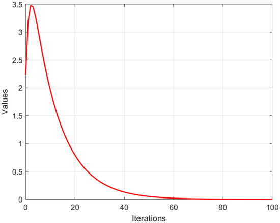
(Two-dimensional specialization). We illustrate our algorithm in the finite-dimensional Banach space $E={\mathbb{R}}^2$ endowed with the standard Euclidean norm and inner product $⟨x,y⟩=x^{\top }y$. The Bregman function is chosen as $h\left(x\right)=\frac{1}{2}{\parallel x\parallel }_2^2,\nabla h\left(x\right)=x,\nabla h^{*}\left(y\right)=y,$ so the associated Bregman distance reduces to ${\mathcal{D}}_h(p,q)=\frac{1}{2}{\parallel p-q\parallel }_2^2.$ We consider two closed convex feasible sets $Q_1=\{d\in {\mathbb{R}}^2:\parallel d-c_1\parallel \le r_1\},Q_2=\{d\in {\mathbb{R}}^2:\parallel d-c_2\parallel \le r_2\},$ with centers $c_1={(0.5,0.2)}^{\top },c_2={(-0.3,-0.4)}^{\top }$ and radii $r_1=1.5,r_2=1.2$. Their intersection $\mathcal{Q}=Q_1\cap Q_2$ is nonempty.

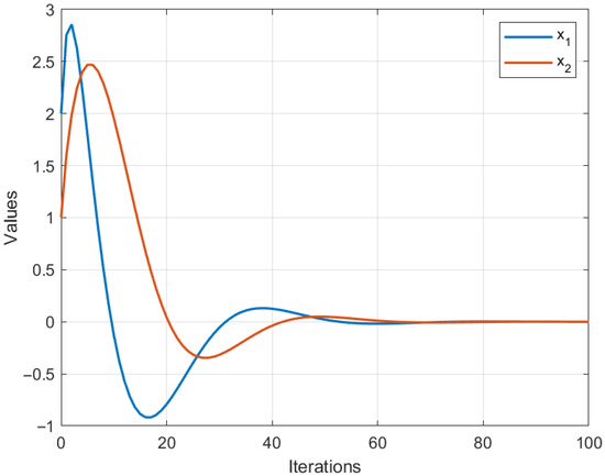
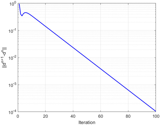
For each $i=1,2$, we define the mappings ${\mathcal{H}}_i(v,z;z)=⟨A_{i}z,v-z⟩,{\mathfrak{f}}_i\equiv 0,$ where $A_1=\left[\begin{array}{cc}1& 0\\ 0& 2\end{array}\right],A_2=\left[\begin{array}{cc}0.8& 0.1\\ 0.1& 1.5\end{array}\right].$ Each $A_i$ is symmetric positive definite; hence, the associated operator is monotone and strongly monotone. The resolvent operator then admits the closed form ${res}_{{\mathcal{H}}_i,b_i}^h\left(u\right)={proj}_{K_i}\left({(I+A_i)}^{-1}u\right).$ For the fixed-point mappings, we consider linear contractions $T_{i1}^n\left(x\right)=B_{i1}x+c_{i1},$ with $B_{11}=0.8I,c_{11}={(0.05,0)}^{\top };B_{21}=0.9\left[\begin{array}{cc}0.99& -0.1\\ 0.1& 0.99\end{array}\right],c_{21}={(-0.02,0.01)}^{\top },$ which are strict contractions and hence asymptotically quasi-nonexpansive in the intermediate sense. The control sequences are chosen as ${\theta }_n={\displaystyle \frac{0.5}{n+1}},{\alpha }_{i0}^n=0.3,{\alpha }_{i1}^n=0.7,{\delta }_i^n=0.5,{\xi }_n\equiv 0,$ all lying in the admissible ranges required by our assumptions. All numerical computations and graphical analyses were implemented in MATLAB R2015(a). Figure 1, Figure 2 and Figure 3 display the convergence behavior with respect to different initial points, the component-wise convergence of iterates, and the error evolution $\parallel d^{n+1}-d^n\parallel$, respectively. The iteration was terminated when $\parallel d^{n+1}-d^n\parallel <{10}^{-10}$.

Figure 1. Convergence of the inertial Bregman algorithm.

Figure 2. Component-wise convergence of the inertial Bregman algorithm.

Figure 3. Error convergence of the inertial Bregman algorithm.

Example 6.

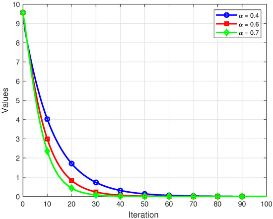
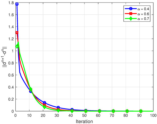
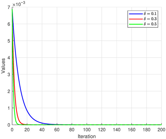
We work in the finite-dimensional Banach space $X={\mathbb{R}}^N$ with the ${\ell }^p$-norm ${\parallel d\parallel }_p={\left({\sum }_{k=1}^N{\left|d_k\right|}^p\right)}^{1/p},p>1$. The Bregman function is $h\left(x\right)={\displaystyle \sum _{i=1}^N}(x_{i}log{x}_i-x_i),x_i>0$, with its gradient $\nabla h\left(x\right)=log\left(x\right)$ and its conjugate $\nabla h^{*}\left(y\right)=exp\left(y\right)$. The feasibility set is given by $\mathcal{Q}=\{x\in {\mathbb{R}}^N:x_i\ge 0,{\displaystyle \sum _i}{x}_i=1\}$, and the projection onto $\mathcal{Q}$ is $\left({\mathrm{proj}}_{\mathcal{Q}}\left(x\right)\right)=\underset{z}{min}{\displaystyle \frac{1}{2}}{\parallel z-x\parallel }_2^2$ such that $z_i>0$, ${\displaystyle \sum _{i=1}}{z}_i=1$.

For each i, we consider the mappings ${\mathcal{H}}_i:Q_i\times Q_i\times Q_i\to \mathbb{R},{\mathcal{H}}_i(v,z;z)=⟨z,v-z⟩,$ and ${\mathfrak{f}}_i:Q_i\times Q_i\to \mathbb{R},{\mathfrak{f}}_i(x,y)=0$. Assume the initial parameter ${\theta }_n=min\{{\displaystyle \frac{1}{n^2\parallel d^n-d^{n-1}\parallel }},0.5\}if{d}^n\ne d^{n-1}$ and otherwise ${\theta }_n=0.5$. In this setting, the associated resolvent reduces to the Bregman projection. The numerical experiments and graphical visualizations were conducted in MATLAB R2015(a). Convergence behavior under different parameter selections is illustrated in Figure 4, Figure 5 and Figure 6. The iterative process was halted when the tolerance $\parallel d^{n+1}-d^n\parallel <{10}^{-10}$ was achieved.

Figure 4. Convergence of the sequence $\left\{d^n\right\}$ for distinct $\alpha$.

Figure 5. Convergence of $\{\parallel d^{n+1}-d^n\parallel \}$ for distinct $\alpha$.

Figure 6. Convergence of the inertial Bregman algorithm for distinct $\delta$.

Algorithm Comparison Summary

We compare our proposed algorithm with Dong et al. [33] (Theorem 3.1). Leveraging adaptive inertia, a larger step size, and an improved operator combination with an additional refinement step, our method consistently outperforms the classical approach, achieving faster early-stage convergence and lower final errors. In Table 1, we describe the structures, whereas, in Table 2 and Figure 7, we show the convergence performance. Overall, our algorithm achieves 2–$5\times$ faster convergence across iterations, demonstrating superior robustness, accuracy, and computational efficiency.

Table 1. Concise comparison between Dong et al. [33] (Theorem 3.1) and our result.

Aspect	Dong et al. [33] (Theorem 3.1)	This Paper/Result
Ambient space	Real Hilbert space H	Real Banach space E with Legendre function h
Problem class	Hierarchical fixed point/VIP	SUGMVLIP: mixed variational-like systems + fixed points
Operators	Nonexpansive mappings ($T,S$)	${\mathcal{H}}_i,{\mathfrak{f}}_i$ (bifunctions) and families ${\mathcal{T}}_{ij}$
Distance/geometry	Euclidean norm; metric projection $P_C$	Bregman distance ${\mathcal{D}}_h$; Bregman projection ${proj}^h$
Resolvent	Not required (or standard monotone resolvent)	Explicit resolvent ${res}_{\mathcal{H},\mathfrak{f}}^h$ per iteration
Convergence target	Strong convergence to $P_{\Gamma }{x}_0$	Strong convergence to ${proj}_{\mathsf{\Theta }}^h\left(d_0\right)$
Computation	Metric projections	Bregman projections/resolvent solves
Relation	Special case when $h\left(x\right)=\frac{1}{2}{\parallel x\parallel }^2$ and $\mathcal{H}\equiv 0$	Generalizes Dong et al.’s result (reduces to it)

Table 2. Iterations to reach error milestones and relative speed-up.

Error	Proposed	Dong et al. [33]	Speed-Up (%)
${10}^{-1}$	5	12	58
$5\times {10}^{-2}$	9	20	55
${10}^{-2}$	18	40	55
$5\times {10}^{-3}$	25	60	58

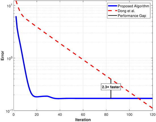
Figure 7. Convergence speed comparison of our result vs. Dong et al. [33].

8. Conclusions

In this paper, we propose a new inertial-type iterative algorithm for finding a common solution of a system of unrelated generalized mixed variational-like inequality problems and the common fixed point of a Bregman asymptotically quasi-nonexpansive mapping in the intermediate sense. Theorems 1 and 2 represent an improvement compared to the results of [3,24,25,28,29,41] in the following sense:

(i)

Iterative Algorithms 1 and 5 are quite different from the iterative algorithm presented in Theorem 3.1 of [24,25,28,29].

(ii)

In [41], the authors proved a strong convergence theorem for a Bregman relatively nonexpansive mapping in a reflexive banach space, whereas, in our Theorem 1, a strong convergence theorem is proved for a Bregman asymptotically quasi-nonexpansive mapping in the intermediate sense.

(iii)

Our result generalizes [3] by proving a strong convergence theorem for Bregman asymptotically quasi-nonexpansive mappings in the intermediate sense in reflexive Banach spaces, extending the earlier result on asymptotically quasi-$\varphi$-nonexpansive mappings in 2-uniformly convex and uniformly smooth spaces.

(iv)

In our results, we need only the generalized relaxed-$\alpha$-monotonicity assumption, which is weaker than monotonicity.

(v)

Theorems 1 and 2 generalize Theorem 1 of [3] by considering duality mappings induced by the Legendre function that are strongly coercive, uniformly Fréchet differentiable, and totally convex.

(vi)

In [28,29], the author considered the fixed-point problem for a Bregman asymptotically quasi-nonexpansive mapping in the intermediate sense, while, in this paper, a system of unrelated generalized mixed variational-like inequality problems and the common fixed point of a Bregman asymptotically quasi-nonexpansive mapping in the intermediate sense are considered.

(vii)

Further, based on the work presented in this paper and the work in [28,29], it is interesting to propose and analyze an iterative scheme for approximating a common solution of these problems without considering the assumption of asymptotic regularity of ${\mathcal{T}}_{ij}$.

References

- Djafari-Rouhani, B.; Kazmi, K.R.; Rizvi, S.H. A hybrid-extragradient-convex approximation method for a system of unrelated mixed equilibrium problems. Trans. Math. Program. Appl. 2013, 8, 82–95. [Google Scholar]
- Kazmi, K.R.; Ali, R. Hybrid projection method for a system of unrelated generalized mixed variational-like inequality problems. Georgian Math. J. 2019, 26, 63–78. [Google Scholar] [CrossRef]
- Farid, M.; Cholamjiak, W.; Ali, R.; Kazmi, K.R. A new shrinking projection algorithm for a generalized mixed variational-like inequality problem and asymptotically quasi-ϕ-nonexpansive mapping in a Banach space. RACSAM 2021, 115, 114. [Google Scholar] [CrossRef]
- Preda, V.; Beldiman, M.; Batatoresou, A. On variational-like inequalities with generalized monotone mappings. In Generalized Convexity and Related Topics, Lecture Notes in Economics and Mathematical Systems; Springer: Berlin/Heidelberg, Germany, 2006; Volume 583, pp. 415–431. [Google Scholar]
- Mahato, N.K.; Nahak, C. Hybrid projection methods for the general variational-like inequality problems. J. Adv. Math. Stud. 2013, 6, 143–158. [Google Scholar]
- Parida, J.; Sahoo, M.; Kumar, A. A variational-like inequality problem. Bull. Aust. Math. Soc. 1989, 39, 225–231. [Google Scholar] [CrossRef]
- Hartman, P.; Stampacchia, G. On some non-linear elliptic differential-functional equation. Acta Math. 1966, 115, 271–310. [Google Scholar] [CrossRef]
- Blum, E.; Oettli, W. From optimization and variational inequalities to equilibrium problems. Math. Stud. 1994, 63, 123–145. [Google Scholar]
- Mahato, N.K.; Noor, M.A.; Sahu, N.K. Existence results for trifunction equilibrium problems and fixed point problems. Anal. Math. Phy. 2019, 9, 323–347. [Google Scholar] [CrossRef]
- Moudafi, A. Second order differential proximal methods for equilibrium problems. J. Inequalities Pure Appl. Math. 2003, 4, 18. [Google Scholar]
- Takahashi, W.; Takeuchi, Y.; Kubota, R. Strong convergence theorems by hybrid methods for families of nonexpansive mappings in Hilbert spaces. J. Math. Anal. Appl. 2008, 341, 276–286. [Google Scholar] [CrossRef]
- Schu, J. Weak and strong convergence to fixed point of asymptotically nonexpansive mapping. Bull. Aust. Math. Soc. 1991, 43, 153–159. [Google Scholar] [CrossRef]
- Inchan, I. Strong convergence theorems of modified Mann iteration methods for asymptotically nonexpansive mappings in Hilbert spaces. Int. J. Math. Anal. 2008, 2, 1135–1145. [Google Scholar]
- Qin, X.L.; Wang, L. On asymptotically quasi-ϕ-nonexpansive mappings in the intermediate sense. Abstr. Appl. Anal. 2012, 2012, 636217. [Google Scholar] [CrossRef]
- Kazmi, K.R.; Ali, R. Common solution to an equilibrium problem and a fixed point problem for an asymptotically quasi-ϕ-nonexpansive mapping in intermediate sense. RACSAM 2017, 111, 877–889. [Google Scholar] [CrossRef]
- Ceng, L.C.; Petrusel, A.; Yao, J.C.; Yao, Y. Hybrid viscosity extragradient method for systems of variational inequalities, fixed Points of nonexpansive mappings, zero points of accretive operators in Banach spaces. Fixed Point Theory 2018, 19, 487–502. [Google Scholar] [CrossRef]
- Ceng, L.C.; Petrusel, A.; Yao, J.C.; Yao, Y. Systems of variational inequalities with hierarchical variational inequality constraints for Lipschitzian pseudocontractions. Fixed Point Theory 2019, 20, 113–133. [Google Scholar] [CrossRef]
- Bregman, L.M. The relaxation method of finding the common point of convex sets and its application to the solution of problems in convex programming. USSR Comput. Math. Phys. 1967, 7, 200–217. [Google Scholar] [CrossRef]
- Bauschke, H.H.; Borwein, J.M.; Combettes, P.I. Essential smoothness, essential strict convexity, and Legendre function in Banach spaces. Comm. Contemp. Math. 2001, 3, 615–647. [Google Scholar] [CrossRef]
- Butnairu, D.; Iusem, A.N. Totally Convex Functions for Fixed Points Computation and Infinite Dimensional Optimization. Applied Optimization; Kluwer Academic: Dordrecht, The Netherlands, 2000; Volume 40. [Google Scholar]
- Reich, S.; Sabach, S. Two strong convergence theorems for a proximal method in reflexive Banach spaces. Numer. Funct. Anal. Optim. 2010, 31, 22–44. [Google Scholar] [CrossRef]
- Agarwal, R.P.; Chen, J.W.; Cho, Y.J. Strong convergence theorems for equilibrium problems and weak Bregman relatively nonexpansive mappings in Banach spaces. J. Ineq. Appl. 2013, 2013, 119. [Google Scholar] [CrossRef]
- Chen, J.W.; Wan, Z.P.; Yuan, L.Y.; Zheng, Y. Approximation of fixed points of weak Bregman relatively nonexpansive mappings in Banach spaces. Int. J. Math. Math. Sci. 2011, 2011, 420192. [Google Scholar] [CrossRef]
- Reich, S.; Sabach, S. Two strong convergence theorems for Bregman strongly nonexpansive operators in reflexive Banach spaces. Nonlinear Anal. 2010, 73, 122–135. [Google Scholar] [CrossRef]
- Suantai, S.; Cho, Y.J.; Cholamjiak, P. Halpern’s iteration for Bregman strongly nanexpansive mappings in reflexive Banach space. Comput. Math. Appl. 2012, 64, 489–499. [Google Scholar] [CrossRef]
- Reich, S. A weak convergence theorem for the alternating method with Bregman distances. In Theory and Applications of Nonlinear Operators; Marcel Dekker: New York, NY, USA, 1996; pp. 313–318. [Google Scholar]
- Reich, S.; Sabach, S. A projection method for solving nonlinear problems in reflexive Banch spaces. J. Fixed Point Theory Appl. 2011, 9, 101–116. [Google Scholar] [CrossRef]
- Tomizawa, Y. A strong convergence theorem for Bregman asymptotically quasi-nonexpansive mappings in the intermediate sense. J. Fixed Point Theory Appl. 2014, 2014, 154. [Google Scholar] [CrossRef]
- Tomizawa, Y. Asymptotically quasi-nonexpansive mappings with respect to Bregman distance in the intermediate sense. Fixed Point Theory 2017, 18, 391–406. [Google Scholar] [CrossRef]
- Maingé, P.E. Convergence theorem for inertial KM-type algorithms. J. Comput. Appl. Math. 2008, 219, 223–236. [Google Scholar] [CrossRef]
- Bot, R.I.; Csetnek, E.R.; Hendrich, C. Inertial Douglas-Rachford splitting for monotone inclusion problems. Appl. Math. Comput. 2015, 256, 472–487. [Google Scholar]
- Dong, Q.L.; Yuan, H.B.; Cho, Y.J.; Rassias, T.M. Modified inertial Mann algorithm and inertial CQ-algorithm for nonexpansive mappings. Optim. Lett. 2018, 12, 87–102. [Google Scholar] [CrossRef]
- Dong, Q.L.; Kazmi, K.R.; Ali, R.; Li, X.H. Inertial Krasnoseski-Mann type hybrid algorithms for solving hierarchical fixed point problems. J. Fixed Point Theory Appl. 2019, 21, 57. [Google Scholar] [CrossRef]
- Khan, S.A.; Suantai, S.; Cholamjiak, W. Shrinking projection methods involving inertial forward-backward splitting methods for inclusion problems. RACSAM 2019, 113, 645–656. [Google Scholar] [CrossRef]
- Liu, L.; Cho, S.Y.; Yao, J.C. Convergence analysis of an inertial Tseng’s extragradient algorithm for solving pseudomonotone variational inequalities and applications. J. Nonlinear Var. Anal. 2021, 5, 627–644. [Google Scholar] [CrossRef]
- Tian, M.; Xu, G. Inertial modified Tseng’s extragradient algorithms for solving monotone variational inequalities and fixed point problems. J. Nonlinear Funct. Anal. 2020, 2020, 35. [Google Scholar] [CrossRef]
- Alansari, M.; Ali, R.; Farid, M. Strong convergence of an inertial iterative algorithm for variational inequality problem, generalized equilibrium problem, and fixed point problem in a Banach space. J. Ineq. Appl. 2020, 2020, 42. [Google Scholar] [CrossRef]
- Kassay, G.; Reich, S.; Sabach, S. Iterative methods for solving systems of variational inequalities in reflexive Banach spaces. SIAM J. Optim. 2011, 21, 1319–1344. [Google Scholar] [CrossRef]
- Alber, Y.I. Metric and generalized projection operators in Banach spaces: Properties and applications. In Theory and Applications of Nonlinear Operators of Accretive and Monotone Type; Dekker: New York, NY, USA, 1996; pp. 15–50. [Google Scholar]
- Butnairu, D.; Resmerita, E. Bregman distances, totally convex functions, and a method for solving operator equations in Banach spaces. Abstr. Appl. Anal. 2006, 2006, 84919. [Google Scholar] [CrossRef]
- Aldosary, S.F.; Cholamjiak, W.; Ali, R.; Farid, M. Strong Convergence of an Inertial Iterative Algorithm for Generalized Mixed Variational-like Inequality Problem and Bregman Relatively Nonexpansive Mapping in Reflexive Banach Space. J. Math. 2021, 2021, 9421449. [Google Scholar] [CrossRef]
Disclaimer/Publisher’s Note: The statements, opinions and data contained in all publications are solely those of the individual author(s) and contributor(s) and not of MDPI and/or the editor(s). MDPI and/or the editor(s) disclaim responsibility for any injury to people or property resulting from any ideas, methods, instructions or products referred to in the content. |
© 2025 by the authors. Licensee MDPI, Basel, Switzerland. This article is an open access article distributed under the terms and conditions of the Creative Commons Attribution (CC BY) license (https://creativecommons.org/licenses/by/4.0/).