Mixed-Integer Linear Programming Models for the Vehicle Routing Problem with Release Times and Reloading at Mobile Satellites

Abstract

The Vehicle Routing Problem (VRP) is central to last-mile logistics, yet a gap remains when products have late release times and vehicles can be reloaded en route via mobile satellites that rendezvous with reloading vehicles at customer locations. We propose the VRP with Release Times and Reloading at Mobile Satellites (VRP-RT-RMS) and develop two mixed-integer linear programming formulations: a three-index (MILP-3) and a two-index (MILP-2). The objective minimizes total distance subject to capacity, route duration, synchronization, and time constraints. We generated 40 instances from real data (10 per size $N\in \{10,15,20,25\}$). En-route reloads simultaneously reduce distance and fleet size and can restore feasibility when the classical VRP is infeasible. To contrast the classical VRP with our VRP-RT-RMS, we analyzed a particular instance with $N=10$ customers: total distance decreased by 7.26% and the number of vehicles fell from 5 to 3. As instance size grows, MILP-2 shows superior scalability and efficiency compared with MILP-3. Beyond the technical scope, coordinating reloads is pertinent to urban operations with late product releases, lowering kilometers traveled and delivery times.

1. Introduction

The Vehicle Routing Problem (VRP) occupies a central place in operations research, shaping decision support for distribution systems and urban freight, and has experienced significant growth in recent decades [1]. Companies seek to optimize routing within their logistics networks to reduce transportation and operating costs, as efficient logistics management and the ability to respond quickly to customer demand are key competitive advantages [2]. In this context, the last mile, the most expensive segment of the supply chain, continues to pose a significant challenge to achieving cost-effective vehicle routing [3]. Moreover, given the wide availability of services, products, and platforms, customers can switch quickly in search of convenience and immediate satisfaction, which raises the requirement for fast and reliable service [4].

A crucial aspect in the VRP is vehicle capacity. When customer demand exceeds vehicle capacity, the number of returns to the central depot increases, resulting in higher operational costs. Another solution to the above is to operate a fleet of own vehicles while having the possibility of using delivery vehicles from a subcontracted company [5]. To mitigate this, several problem variants have been developed. Among them is the Feeder Vehicle Routing Problem (FVRP) [6], which considers the use of additional vehicles or en-route reloading when demand exceeds the capacity of a single vehicle, thereby reducing total transportation costs. The Real-Time VRP (RTVRP) [7] addresses dynamic and uncertain scenarios typical in logistics, where request changes and time windows are considered, making it especially relevant in urban settings. The Collaborative VRP (CVRP) [8] proposes cooperation among multiple logistics companies that share fleets and jointly plan routes to optimize resources and reduce operational costs. The Line-Haul Feeder Vehicle Routing Problem (LFVRP) [9] combines large-capacity vehicles that supply smaller vehicles en-route, avoiding the need to return to the central depot and improving transportation efficiency. Additionally, the Vehicle Routing Problem with Release Times (VRP-RT) [10] incorporates product availability constraints through release times, and the Inventory Routing Problem with Satellite Facilities (IRPSF) [11] integrates inventory management with routing optimization, using satellite depots to replenish vehicles in the field. Related to these variants, there is still a gap in the literature regarding VRPs with mobile satellite facilities [12] and cross-docking operations [13], particularly in en-route reloading to avoid unnecessary returns to the depot. In this context, key objectives include integrating cross-docking operations with optimal vehicle routing and ensuring synchronization between two entities (e.g., supplier–customer), so that both collaborate simultaneously in the physical inbound and outbound flows at each transshipment point [2]. This gap represents one of the most relevant research trends in the field [14].

This study proposes a new variant of the Vehicle Routing Problem called Vehicle Routing Problem with Release Times and Reloading at Mobile Satellites (VRP-RT-RMS), which considers reloading at mobile satellites for delivery vehicles already en-route as part of last-mile distribution logistics. The products demanded by customers are classified into two categories: early-release (available from the start of planning) and late release (not interchangeable with the former). Availability depends on the central depot, where early-release products are ready at the beginning, while late release products are still in manufacturing and will only become available after routes have started. Unlike the traditional VRP, the proposed model allows en-route reloads at mobile satellites instead of forcing vehicles to return to the depot, Figure 1 contrasts both settings (VRP vs. VRP with reload). Compared with the VRP with Release Times (VRP-RT), where late-release products can only be loaded at the depot, leading to waits or depot returns, VRP-RT-RMS enables en-route reloads via mobile satellites that meet delivery vehicles at customer locations, allowing multiple reloads within a single route. To handle late-release products, a reload vehicle transports them to mobile satellites, where cross-docking is performed; in the route design, these satellites coincide with selected customer locations (either early-release or late-release customers) and act as temporary cross-docking points, so delivery vehicles need not return to the depot. Operationally, delivery vehicles that depart before the late-release time leave with early-release products only and may later be en-route reloaded by the reload vehicle with late-release products; delivery vehicles that depart after the late-release time can carry both early- and late-release products from the depot and may also receive en-route reloads of late-release products. The model aims to minimize the total distance traveled by all vehicles, subject to capacity constraints, synchronization at mobile satellites, maximum route duration, and the condition that the reloading vehicle can only depart after late release products become available.

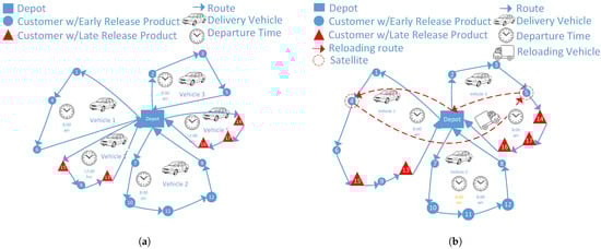
Figure 1. (a) Describe the operation of late-release product deliveries in a traditional VRP. (b) Describe the operation of late-release product deliveries in a VRP with the possibility of en-route reloading.

The main contributions and novel aspects of this study are summarized as follows:

• We propose a new variant of the Vehicle Routing Problem, the Vehicle Routing Problem with Release Times and Reloading at Mobile Satellites (VRP-RT-RMS), which jointly integrates late product availability and en-route reloading operations.
• The models explicitly incorporate synchronization between the reloading vehicle and the delivery vehicles at customer nodes that act as mobile satellites.
• A realistic instance generation procedure is designed based on real-world last-mile delivery data from Santiago, Chile, preserving spatial and demand distributions.
• Comprehensive computational experiments are conducted to evaluate the models’ performance, and solution quality, showing that MILP-2 achieves higher efficiency and smaller optimality gaps.
• The results show operational benefits over the classical VRP, including reduced total distance, fleet utilization, and idle time, highlighting the practical value of integrating in-route reloading.

The remainder of the paper is organized as follows. Section 2 reviews related work on en-route reload, satellite-based transfer/cross-docking, and release times. Section 3 defines the VRP-RT-RMS and states the modeling assumptions. Section 4 presents two mixed-integer linear programming formulations, MILP-3 (three-index) and MILP-2 (two-index), together with their constraints. The Section 5, first details the instance generation in Section 5.1, then presents the computational analysis in Section 5.2, and subsequently examines fleet usage and reloading patterns in Section 5.3. Finally, Section 6 concludes and outlines avenues for future research.

2. Literature Review

Our study presents a new variant, the Vehicle Routing Problem with Release Times and Reloading at Mobile Satellites (VRP-RT-RMS), a VRP variant that combines en-route reloading via mobile satellites with release times. We explicitly assume a heterogeneous fleet composed of one high-capacity reloading vehicle and multiple identical, limited-capacity delivery vehicles; at mobile satellites located at selected customer nodes, the delivery vehicles rendezvous with the reloading vehicle to perform cross-docking and reloading operations, all subject to capacity, synchronization, and maximum route duration constraints. We then survey the literature in three groups: the first ten studies address problems that allow en-route reload; the next group focuses on the use of satellites for transfer/cross-docking; and, finally, we review works that emphasize release times.

Huang et al. [6] introduce the Feeder Vehicle Routing Problem (FVRP), where trucks act as mobile depots and limited-capacity motorcycles reload at joint nodes from an assigned truck, minimizing total cost (fixed and travel) and explicitly incorporating travel, service, waiting, and reloading times, as well as the decision on the number of supporting sub-fleets required. Subsequently, Sarbijan and Behnamian [15] propose the Multi-Fleet FVRP, which, unlike Huang et al. [6], does not restrict the reload to a single truck, allowing a motorcycle to meet multiple trucks at different joints. To solve the proposed problems, Huang et al. [6] use Ant Colony Optimization (ACO), whereas Sarbijan and Behnamian [15] formulate a MILP and tackle it with PSO and a hybrid PSO-SA.

Earlier, Ref. [16] introduced the Line-haul Feeder Vehicle Routing Problem with Virtual Depots (LFVRP-VD), considering a fleet composed of one large vehicle (truck) and several small units (bicycles or motorcycles), and two customer types: type-I customers, which can serve as Virtual Depots (VDs), and type-II customers, which are only accessible by small vehicles. In this setting, small vehicles can reload either from the truck or from the Physical Depot (PD), aiming to minimize the total travel and waiting costs. In a related study, Chen et al. [17] extended the problem to the LFVRP with hard time windows (LFVRPTW), incorporating driver shift limits and synchronization between vehicle classes. Their model allows reloading at the PD or at VDs when both vehicles coincide in time and space, minimizing fixed and travel costs through a two-stage heuristic with Tabu Search. These contributions by [16,17], established the foundation for subsequent research on synchronized line-haul–feeder systems. Building on this line of work, Brandstätter and Reimann [18] revisited the LFVRP and proposed two dedicated improvement heuristics—the Linkage and Split Approaches—based on the analysis of illustrative examples that highlight the benefits of transshipment at customer nodes. Their results showed that allowing in-route reloads at customer locations can reduce total distance by around $25\%$ and decrease the number of small vehicles required compared with the classical VRP. Subsequently, Brandstätter [19] studied the LFVRPTW while maintaining the synchronization and virtual-depot logic established by Chen et al. [17], but improving solution quality through a multi-start matheuristic based on the Linkage Approach. In contrast to the earlier constructive heuristics of Chen et al. [16], their method explicitly exploits time-window synchronization to enhance route feasibility and computational performance.

Expanding upon this research stream, Chen and Wang [20] addressed the Extended Line-haul Feeder Vehicle Routing Problem with Time Windows (ELFVRPTW), which generalizes the LFVRPTW by incorporating multiple large-capacity trucks (line-haul vehicles) of limited capacity instead of a single unrestricted one. In this variant, each large vehicle can serve as a mobile depot for several small delivery units, maintaining variable Virtual Depots (VDs), hard time windows, and driver shift limits, while explicitly considering capacity constraints for both vehicle types. The objective function was broadened to include fixed, travel, labor, and waiting costs, thus capturing a more comprehensive operational perspective. The authors proposed a two-stage heuristic procedure—first constructing feasible routes and then improving them through local search—and demonstrated that their approach achieved better average objective values and required fewer vehicles than previous LFVRPTW heuristics under comparable test conditions.

Sarbijan and Behnamian [21] formulate the Real-Time Feeder Vehicle Routing Problem (RTFVRP), a dynamic VRP where customer requests arrive over time without prior knowledge. The model considers a heterogeneous fleet of trucks and motorcycles that can dynamically pair at joint nodes, enabling real-time coordination between feeder and delivery vehicles. To solve it, the authors develop a Mixed-Integer Linear Programming (MILP) model and a Dynamic Inertia Weight Particle Swarm Optimization (DIWPSO) algorithm to balance computation time and routing cost. Experiments on dynamic benchmarks show that the DIWPSO outperforms Differential Evolution (DE) in both cost and runtime, achieving over $30\%$ cost reductions compared with static settings. Following this, Sarbijan and Behnamian [22] extend the framework to a Real-Time Collaborative Feeder Vehicle Routing Problem (RTCFVRP) with flexible time windows and inter-company cooperation, where two depots share heterogeneous fleets. They propose a MILP model solved via the augmented $\epsilon$-constraint method and two metaheuristics: MOPSO and MOPSO–VNS, the latter yielding superior Pareto fronts and scalability over NSGA-II and MOEA/D under static and dynamic scenarios.

For their part, Ref. [23] present a CFVRP with flexible time windows (CFVRPFlexTW) in a collaborative, bi-objective setting (minimizing costs and maximizing satisfaction), addressing a static collaborative scenario with MOPSO variants (WMOPSO/LAMOPSO) and an explicit FVRP+CVRP combination. This study also presents a MILP solved with AEC/CPLEX, and develops WMOPSO (MOPSO with dynamic inertia) and LAMOPSO (MOPSO with an adaptive learning strategy).

Regarding freight transfer via satellites, the term satellite refers to a fixed transshipment point for transferring products from one vehicle to another, without storage capacity, as used in the research by [24], which connects first- and second-echelon distribution flows [14]. This concept differs from feeders, where transfers occur dynamically between vehicles en route. Bard et al. [11] study the Inventory Routing Problem with Satellite Facilities (IRPSF) under demand uncertainty, in which satellites with storage capacity serve as intermediate reload points that extend vehicle tours without requiring a return to the central depot. Subsequent studies have adopted satellites to perform freight transfers without temporary storage, typically through cross-docking processes. For instance, Maknoon et al. [25] focus on scheduling transshipment operations in a satellite cross-dock, conceived as an intermediate facility where inbound trucks unload products, transfer them to outbound vehicles, and these complete final deliveries to customers. Similarly, Li et al. [26] address the Two-Echelon Vehicle Routing Problem with Time Windows in Line-Haul Delivery Systems (2E-TVRP), where urban peripheral centers are connected to satellites that, in turn, link to end customers. Bevilaqua et al. [24] examine the Two-Echelon Fixed Fleet Heterogeneous Vehicle Routing Problem (2E-HVRP), where freight is transferred between vehicles belonging to different heterogeneous fleets via a satellite. Likewise, Mühlbauer and Fontaine [27] define satellites as meeting points in the Two-Echelon Capacitated Vehicle Routing Problem (2E-CVRP), employing cross-docking between vans and cargo bikes through exchange containers to avoid direct product handling. More recently, Yang and Wang [28] investigate the Two-Echelon Capacitated Vehicle Routing Problem with Backhauls (2E-CVRP-B), where the first echelon transports freight from the depot to satellites and the second echelon serves customers. Taken together, these studies illustrate the conceptual evolution of satellites—from static storage facilities to dynamic cross-docking transshipment nodes. However, none of them address mobile or real-time satellite operations, and their applications remain confined to two-echelon distribution systems, where routes are decomposed to optimize last-mile delivery performance.

Regarding release time characteristics, this class of problems incorporates temporal availability constraints, where customer orders or shipments become serviceable only after a specified release time. Unlike feeder or satellite-based systems that focus on spatial coordination between vehicles or facilities, release-time problems emphasize temporal synchronization between order readiness and vehicle dispatch. For example, Babagolzadeh et al. [29] develop a model applied to airport operations in Australia, where major metropolitan terminals are nearing their capacity limits, while regional airports remain underutilized. The model considers a heterogeneous fleet for distribution, with fuel consumption depending on load, distance, speed, and vehicle characteristics. Furthermore, the release time is defined as the time required for the cargo to be ready for delivery at a destination airport. Torres-Tapia et al. [10] study a VRP with release times (VRP-RT), in which an infinite-capacity fleet departs periodically every h hours from the factory and returns after each tour. They formulate a MILP and propose a hybrid Iterated Local Search with Variable Neighborhood Descent (ILS-VND) to minimize total routing cost. Subsequently, Xue and Wang [30] address order acceptance and scheduling in instant delivery as an MT-PCPDP with release and deadline times (RT&DT), decomposing the dynamic problem into static subproblems solved at discrete intervals. Their approach, based on the Online Insertion if Beneficial–Trajectory Similarity Optimization (OIB-TSO) policy, yields efficient multi-trip routing plans without reloads or satellites. While these studies capture the timing dimension of routing decisions, they overlook synchronization between dynamically released orders and reloading or collaborative mechanisms—an interaction addressed in the present work.

To address these combined spatial–temporal synchronization challenges, this study proposes the VRP-RT-RMS, a model that integrates real-time order release, mobile satellite reloading, and inter-fleet coordination within a unified routing framework.

In comparison with previous studies, and as summarized in Table 1, our work tackles a VRP variant that enables en-route reloads for late-release products using mobile satellites. Prior research can be grouped into three main categories: (i) papers that enable reload en-route, e.g., trucks as mobile depots or VDs at customers [6,15,16,17,18,19,20], but do not model release times; (ii) satellite-based transfer studies [11,24,25,26,27,28], which employ fixed satellites—either as cross-docking facilities without storage or as satellite depots with limited storage—but do not consider release times nor target en-route reloads for late-release products; and (iii) release-time works [10,29,30], which schedule operations based on release times but do not permit en-route reloads and do not employ mobile satellites.

Table 1. Summary of the main features of the reviewed studies on VRP with release times and reloading.

Authors	Problem	Reloading	Release Time	Fleet	Satellite	Solution Method
[6]	FVRP	Yes	No	Heterogeneous	No	ACO
[15]	Multi-Fleet FVRP	Yes	No	Heterogeneous	No	PSO PSO–SA
[18]	LFVRP	Yes	No	Heterogeneous	No	Linkage/ Split
[16]	LFVRP-VD	Yes	No	Heterogeneous	No	Cost-sharing Threshold
[19]	LFVRPTW	Yes	No	Heterogeneous	No	Linkage-based matheuristic (multi-start + local search)
[17]	LFVRPTW	Yes	No	Heterogeneous	No	Tabu Search
[20]	ELFVRPTW	Yes	No	Heterogeneous	No	Two-stage
[21]	RTFVRP	Yes	No	Heterogeneous	No	DIWPSO
[22]	RTCFVRP	Yes	No	Heterogeneous	No	MOPSO MOPSO-VNS
[23]	CFVRPFlexTW	Yes	No	Heterogeneous	No	WMOPSO LAMOPSO
[11]	IRPSF	Yes	No	Homogeneous	Yes	Randomized Clarke–Wright GRASP Modified sweep
[25]	satellite cross-dock	Yes	No	Homogeneous	Yes	Sequential priority-based heuristic
[26]	2E-TVRP	Yes	No	Homogeneous	Yes	Clarke–Wright Local Search phase
[24]	2E-HVRP	Yes	No	Heterogeneous	Yes	Parallel island based Memetic Algorithm Lin–Kernighan local search
[27]	2E-CVRP	Yes	No	Heterogeneous	Yes	Parallelised large neighbourhood search
[28]	2E-CVRP-B	Yes	No	Heterogeneous	Yes	RePart-DRL (DRL + LNS)
[29]	OVRP	No	Yes	Heterogeneous	No	Exact
[10]	VRP-RT	No	Yes	Homogeneous	No	Hybrid ILS–VND
[30]	OAS-IDS MT-PCPDP- RT&DT	No	Yes	Homogeneous	No	Online insertion OIB-TSO
Current Study	VRP-RT-RMS	Yes	Yes	Heterogeneous	Yes	Exact

Table 1 summarizes the key studies reviewed in this section, organized according to whether they address en-route reloading, satellite-based transfer, or release-time constraints. Additional related works are also referenced in the text but omitted from the table for conciseness. In contrast, VRP-RT-RMS jointly models late-release products, en-route reloads at mobile satellites that coordinate with vehicles at customer locations, enforces synchronization driven by release times, allows multiple reloads within a single route, and operates with a heterogeneous fleet, thereby providing the integrated capability missing in previous literature.

3. Description of the Problem

Let $Np$ and $LRp$ denote the numbers of early-release and late-release customers, respectively. Formally, we define the VRP-RT-RMS as a complete graph with node set $N=\{0,\dots ,Np,Np+1,\dots ,Np+LRp\}$, where node 0 denotes the central depot and the remaining nodes denote customer locations. The time horizon is bounded by $Tmax$, defined as the maximum route duration time. We use $Pr=1$ to denote early-release products and $Pr=2$ to denote late-release products. The customer set $C=\{1,\dots ,Np,Np+1,\dots ,Np+LRp\}$ is partitioned into two categories:

• $ER=\{1,\dots ,Np\}$: customers requesting early-release products $(Pr=1)$, available at the depot from the start of the planning horizon $(t=0)$.
• $LR=\{Np+1,\dots ,Np+LRp\}$: customers requesting late-release products $(Pr=2)$, available only after the release time $Rt$.

The customers $i\in ER$ have demand for product type-1 $\left(Dem{P}_{i1}\right)$. Each customer $i\in LR$ has a mandatory demand $Dem{P}_{i2}$ for product type-2, and may have an optional demand $Dem{P}_{i1}$ for product type-1. Demands for type-1 and type-2 products are not interchangeable and must be satisfied separately. If a customer requests both types of products, it is classified in $LR$ due to delivery time constraints.

A fleet of k delivery vehicles is available, each with capacity $Qv$, along with a reloading vehicle with capacity $Qt$, which is assumed to be sufficiently large compared with the total demand for product type-2, ensuring that reloading operations are not limited by its capacity. All vehicles start and end their routes at the depot. Delivery vehicles depart from the depot carrying only products of type $Pr=1$. After the release time $Rt$, the reloading vehicle departs carrying all products of type $Pr=2$ and can meet the delivery vehicles at a feasible mobile satellite point along the route. Mobile satellites may be any customer node $j\in C$. Since the chosen satellite is also a customer to be served, service and reloading can take place during the same stop, provided they are synchronized. This meeting, if reloading is required, may occur before or at the first delivery of a type-2 product on the route, preventing delivery vehicles from having to return to the depot. Reloading occurs when the delivery vehicle and the reloading vehicle arrive simultaneously at the same mobile satellite. The reloading operation has a fixed duration of $Tr$ minutes. Each customer is visited exactly once by a single delivery vehicle, with a fixed service time of $St$ minutes. The reloading vehicle does not deliver directly to customers. Moreover, delivery vehicles can be reloaded multiple times with type-2 product along a single route.

We set $Rt$, assuming production of $Pr=2$ items finishes around mid-shift, so their effective availability coincides with the midpoint of the planning horizon T (maximum route duration). Let $T_{ij}$ and $Di{s}_{ij}$ denote the travel time and distance between nodes i and j, respectively; the service time at each customer is $St$. The objective is to determine the routes of the delivery vehicles and the reloading vehicle such that

• All demands for products $Pr=1$ and $Pr=2$ are satisfied;
• Vehicle capacities are respected;
• Each customer is visited exactly once by a single delivery vehicle;
• Mobile satellites are selected among ER/LR customers at feasible nodes occurring after $Rt$, enabling reloading before or at the first type-2 delivery; multiple reloads per route are permitted;
• Synchronization at reloading points is guaranteed;
• The total distance traveled by all vehicles (delivery and reloading) is minimized.

Figure 1 illustrates the operational difference between the traditional VRP and the proposed VRP-RT-RMS. Figure 1a represents the traditional scheme, in which delivery vehicles depart from the depot carrying products available from the beginning of the planning horizon ($t=0$), referred to as Early Release Products (type-1). To deliver Late Release Products (type-2), which become available only after $R_t$, vehicles must either wait at the customer location or return to the depot for reloading, thereby increasing both the total distance traveled and the idle time at the depot. Figure 1b shows the proposed en-route reloading approach, where, in addition to the delivery routes, a reloading route (dashed line) is incorporated. This reloading vehicle departs only when $t\ge R_t$, carrying type-2 products, and coordinates with delivery vehicles at selected mobile satellites, which coincide with customer nodes. At these points, a transfer (cross-docking) operation is carried out under synchronized timing, allowing delivery vehicles to continue their routes without returning to the depot. The comparison between both schemes clearly demonstrates that the proposed VRP-RT-RMS model achieves a significant reduction in total distance traveled and idle time, thereby improving operational efficiency and fleet utilization—particularly in scenarios with a high proportion of late-release products.

4. Proposed Mathematical Models

Below, we present a mixed-integer linear programming (MILP) formulation in two variants. First, we develop a three-index model (MILP-3) that explicitly represents vehicle movements, load variables, and travel times. This formulation details the routing of the delivery vehicles and the reloading vehicle, capacity usage by product type, reloading at satellite nodes, synchronization between the reloading vehicle and the delivery vehicles, and compliance with product release times. Second, we propose a two-index model (MILP-2) that lowers dimensionality by dropping the vehicle index from the routing variables while preserving flow conservation, the selection of reloading satellites, capacity constraints by product type, temporal constraints (travel and service), synchronization, and compliance with release times. Both models share the same sets and parameters.

Both models share the same sets and parameters and are developed under the following assumptions:

• All vehicles start and end their routes at the central depot.
• The delivery vehicle fleet has a limited capacity $Q_v$, while the reloading vehicle has a sufficiently large capacity $Q_t$ to satisfy the total demand for type-2 products.
• Products are classified into two non-interchangeable types: early-release (type-1) and late-release (type-2).
• Travel times, service times, and reloading times are deterministic and known.
• Mobile satellite points coincide with customer locations and operate as temporary cross-docking points without storage capacity.
• Synchronization between the reloading vehicle and the delivery vehicle at a mobile satellite is assumed to be perfect; both must coincide spatially and temporally for the reloading operation to occur.
• Each customer is served exactly once by a single delivery vehicle.
• The reloading vehicle does not deliver directly to customers.
• The release time is the same for all type-2 products.
• All routes must be completed within a maximum time horizon $Tmax$.

Below, we present the sets and parameters common to both models, which define the notation used in the mathematical formulations:

• Sets

• $N=\{0,\dots ,Np,Np+1,\dots ,Np+LRp\}$: Set of nodes of all customers, including both early-release and late-release customers. Includes the depot (0).
• $ER=\{1,\dots ,Np\}$: Set of customers requesting only early-release products.
• $\mathit{ER}\mathit{0}=\{0,\dots ,Np\}$: Set of customers requesting only early-release products, including the depot.
• $LR=\{Np+1,\dots ,Np+LRp\}$: Set of customers requesting late-release products.
• $C=ER\cup LR$: Set containing all customers.
• $K=\{1,\dots ,Kp\}$: Set of the total delivery vehicles available.
• $Pr=\{1,2\}$: Set including early-release products (type-1) and late-release products (type-2).

• Parameters

• $Np$: Number of customers with early product release time (u).
• $LRp$: Number of customers with late product release time (u).
• $Kp$: Number of delivery vehicles (u).
• $Di{s}_{ij}$: Distance between nodes $i\in N$ and $j\in N$ (m).
• $T_{ij}$: Travel time from $i\in N$ to $j\in N$ (min).
• $Dem{P}_{ip}$: Demand of node $i\in N$ for product $p\in Pr$ (u).
• $Qt$: Reloading vehicle capacity (u).
• $Qv$: Delivery vehicle capacity (u).
• $Tmax$: Maximum route duration time (min).
• $St$: Service time (min).
• $Tr$: Reloading time (min).
• $Rt$: Late product release time (min).

4.1. Mathematical Model of Three Index

• Decision Variables

• $x_{ij}=\left\{\begin{array}{cc}1,\hfill & \mathrm{if}\mathrm{the}\mathrm{reloading}\mathrm{vehicle}\mathrm{travels}\mathrm{from}\mathrm{node}i\in N\mathrm{to}\mathrm{node}j\in N\hfill \\ 0,\hfill & \mathrm{otherwise}\hfill \end{array}\right.$
• $y_{ijk}=\left\{\begin{array}{cc}1,\hfill & \mathrm{if}\mathrm{the}\mathrm{delivery}\mathrm{vehicle}k\in K\mathrm{travels}\mathrm{from}\mathrm{node}i\in N\mathrm{to}\mathrm{node}j\in N\hfill \\ 0,\hfill & \mathrm{otherwise}\hfill \end{array}\right.$
• $w_{jk}=\left\{\begin{array}{cc}1,\hfill & \mathrm{if}\mathrm{the}\mathrm{node}j\in N\mathrm{is}\mathrm{a}\mathrm{satellite}\mathrm{for}\mathrm{delivery}\mathrm{vehicle}k\in K\hfill \\ 0,\hfill & \mathrm{otherwise}\hfill \end{array}\right.$
• $f_{ikp}$: freight transported of product $p\in Pr$ by delivery vehicle $k\in K$ before visiting node $i\in N$ (u).
• $c_i$: time of arrival of the reloading vehicle at node $i\in N$ (min).
• $a_{ik}$: time of arrival of the delivery vehicle $k\in K$ at node $i\in N$ (min).
• $l{e}_k=\left\{\begin{array}{cc}1,\hfill & \mathrm{if}\mathrm{the}\mathrm{delivery}\mathrm{vehicle}k\in K\mathrm{departs}\mathrm{from}\mathrm{the}\mathrm{depot}\mathrm{at}\mathrm{or}\mathrm{after}Rt\hfill \\ 0,\hfill & \mathrm{if}\mathrm{it}\mathrm{departs}\mathrm{before}Rt\hfill \end{array}\right.$
• $d{t}_k$: departure time of vehicle $k\in K$ from the depot (min)

• Objective Function

$$\mathrm{minimize}z=\sum _{i\in \mathit{N}}\sum _{\begin{array}{c}j\in \mathit{N}\\ j\ne i\end{array}}Di{s}_{ij}·x_{ij}+\sum _{k\in K}\sum _{i\in N}\sum _{\begin{array}{c}j\in N\\ j\ne i\end{array}}Di{s}_{ij}·y_{ijk}$$

(1)

The objective function (Equation (1)) minimizes the total distance traveled by the reloading vehicle and delivery vehicles.

• Subject to

• Flow of Reloading reloading vehicle

  $$\sum _{\begin{array}{c}j\in \mathit{N}\\ j\ne i\end{array}}{x}_{ij}\le 1,\forall i\in N$$

  (2)

  $$\sum _{\begin{array}{c}i\in \mathit{N}\\ i\ne l\end{array}}{x}_{il}=\sum _{\begin{array}{c}j\in \mathit{N}\\ j\ne l\end{array}}{x}_{lj},\forall l\in N$$

  (3)

  $$\sum _{i\in C}{x}_{0i}\le 1$$

  (4)
• Flow of Delivery Vehicles

  $$\sum _{\begin{array}{c}k\in K\end{array}}\sum _{\begin{array}{c}j\in N\\ j\ne i\end{array}}{y}_{ijk}=1,\forall i\in C$$

  (5)

  $$\sum _{j\in C}{y}_{0jk}\le 1,\forall k\in K$$

  (6)

  $$\sum _{\begin{array}{c}k\in K\end{array}}\sum _{\begin{array}{c}i\in N\\ j\ne i\end{array}}{y}_{ijk}=1,\forall j\in C$$

  (7)

  $$\sum _{\begin{array}{c}i\in N\\ i\ne l\end{array}}{y}_{ilk}=\sum _{\begin{array}{c}j\in N\\ j\ne l\end{array}}{y}_{ljk},\forall l\in N,k\in K$$

  (8)
  Constraints (2)–(8) ensure the flow balance across all vehicles. In particular, constraints (2)–(4) the route of the reloading vehicle from the depot to the customers. Constraints (5)–(8) establish the routing of the delivery vehicles.
• Reloading Nodes

  $$\sum _{\begin{array}{c}i\in \mathit{N}\\ j\ne i\end{array}}{x}_{ij}\ge w_{jk},\forall j\in C,k\in K$$

  (9)
  Constraint (9) ensures that if node j is designated as a reloading satellite for some delivery vehicle k, then the reloading vehicle must travel to node j from some preceding node i.

  $$\sum _{\begin{array}{c}i\in N\\ j\ne i\end{array}}{y}_{ijk}\ge w_{jk},\forall j\in C,k\in K$$

  (10)
  Constraint (10) ensures that if node j is selected as a reloading satellite, then it must be visited by a delivery vehicle.

  $$\sum _{\begin{array}{c}i\in \mathit{N}\\ j\ne i\end{array}}{x}_{ij}+\sum _{\begin{array}{c}i\in N\\ j\ne i\end{array}}{y}_{ijk}\le w_{jk}+1,\forall j\in C,k\in K$$

  (11)
  Constraint (11), together with constraints (9) and (10), ensures that if both the reloading vehicle and delivery vehicle k visit node j (i.e., when ${\sum }_i{x}_{ij}=1$ and ${\sum }_i{y}_{ijk}=1$), then node j must be designated as a reloading satellite ($w_{jk}=1$).

  $$\sum _{k\in K}{w}_{jk}\le 1,\forall j\in C$$

  (12)
  Constraint (12) states that, although any node j can be selected as a satellite, each satellite can be assigned to at most one delivery vehicle. Together with constraints (9)–(11), it guarantees that the selected satellites are visited by both vehicles and that the meeting takes place at that node.
• Reloading
  Constraints (13)–(15) regulate the freight capacity of delivery vehicles along the routes.

  $$\sum _{p\in Pr}{f}_{ikp}\le Qv,\forall i\in N,k\in K$$

  (13)
  Constraint (13) ensures that, before visiting any node i, the sum of the freight carried by delivery vehicle k across both product types never exceeds the maximum delivery vehicle capacity $Qv$.

  $$f_{jk2}\le f_{ik2}-Dem{P}_{i2}+Qt·(1-y_{ijk}+w_{ik}),\forall i\in C,j\in N,k\in K,j\ne i$$

  (14)
  Constraint (14) ensures load conservation for product type-2 while accounting for both deliveries and possible en-route reloads. When $y_{ijk}=1$ and $w_{ik}=0$, vehicle k travels from node i to node j, so the load before visiting j ($f_{jk2}$) must be less than or equal to the load before visiting i ($f_{ik2}$) minus the demand served at i ($Dem{P}_{i2}$). However, if node i operates as a satellite $w_{ik}=1$, the term $Qt·(1-y_{ijk}+w_{ik})=Qt·(1-1+1)$ allows the load to increase up to the reloading vehicle’s capacity, representing a reloading operation. Thus, the constraint distinguishes three situations: normal unloading $y_{ijk}=1,w_{ik}=0$, reloading at a satellite $y_{ijk}=1,w_{ik}=1$, and inactive arcs $y_{ijk}=0$, ensuring a consistent and physically feasible load flow throughout the route.

  $$f_{jk1}\le f_{ik1}-Dem{P}_{i1}+Qv·(1-y_{ijk}),\forall i\in C,j\in N,k\in K,j\ne i$$

  (15)
  Constraint (15) establishes the analogous conservation rule for product type-1 (early release), where no reloading is permitted along the route. Thus, if an arc $i,j$ is used, the load before visiting j must not exceed the load before visiting i minus the demand at i. The parameter $Qv$, similarly to $Qt$ in Constraint (14), acts as a $Big-M$ constant, ensuring that the constraint is relaxed whenever the arc $(i,j)$ is not part of the route ($y_{ijk}=0$).
• Reloading Vehicle Time Constraints

  $$c_i\le Tmax,\forall i\in \mathit{N}$$

  (16)

  $$c_j\ge c_i+T_{ij}+Tr-Tmax·(1-x_{ij})\forall i\in C,j\in \mathit{N},j\ne i$$

  (17)

  $$c_j\ge T_{0j}-Tmax·(1-x_{0j})\forall j\in C$$

  (18)
• Delivery Vehicle Time Constraints

  $$a_{jk}\le Tmax,\forall j\in N,k\in K$$

  (19)

  $$a_{jk}\ge a_{ik}+T_{ij}+St-Tmax·(1-y_{ijk}),\forall i\in C,j\in N,k\in K,j\ne i$$

  (20)

  $$a_{jk}\ge T_{0j}-Tmax·(1-y_{0jk}),\forall j\in C,k\in K$$

  (21)
  Constraints (16)–(18) control the routing time of the reloading vehicle, ensuring that the maximum route duration is not exceeded and that the temporal sequence of visits between nodes, including reloading times, is preserved. Similarly, constraints (19)–(21) regulate the accumulated time of the delivery vehicles, also accounting for customer service times.
• Synchronization

  $$a_{jk}\ge c_j-Tmax·(1-w_{jk}),\forall j\in C,k\in K$$

  (22)

  $$c_j\ge a_{jk}-Tmax·(1-w_{jk}),\forall j\in C,k\in K,j\ne i$$

  (23)
  Constraints (22) and (23) correspond to the synchronization between the reloading vehicle and the delivery vehicles, establishing that if a node operates as a satellite ($w_{jk}=1$), the arrival time of the delivery vehicle must match the arrival time of the reloading vehicle.
• Release Time
  Constraints (24)–(29) ensure compliance with the release times of late-release products.

  $$c_j\ge Rt+T_{0j}·x_{0j},\forall j\in C$$

  (24)
  Constraint (24) ensures that the reloading vehicle does not reach a customer before the product release time plus the travel time from the depot to the first customer. Specifically, if j is the first customer (i.e., $x_{0j}=1$, the constraint enforces $c_j\ge Rt+T_{0j}$; otherwise, it reduces to $c_j\ge Rt$), thus preventing any visit prior to the release.

  $$d{t}_k\ge Rt-Tmax·(1-l{e}_k),\forall k\in K$$

  (25)

  $$d{t}_k\le Rt-ϵ+Tmax·l{e}_k,\forall k\in K$$

  (26)
  Constraints (25) and (26) form a pair of dichotomous constraints that regulate the departure time of delivery vehicle k with respect to the product release time $Rt$. Only one of them is active depending on the value of the binary variable $l{e}_k$. When $l{e}_k=1$, Constraint (25) becomes active, resulting in $d{t}_k\ge Rt$; this indicates that the delivery vehicle departs at or after the release time, corresponding to a late-departure scenario. Conversely, when $l{e}_k=0$, Constraint (26) is activated, yielding $d{t}_k\le Rt-ϵ$; in this case, the delivery vehicle departs before the release time, representing an early-departure scenario. The parameter $ϵ>0$ prevents numerical ambiguities between the two cases, while T acts as a $Big-M$ constant that deactivates the constraint not applicable for the given value of $l{e}_k$.

  $$d{t}_k\ge a_{jk}-T_{0j}-Tmax·(1-y_{0jk}),\forall j\in C,k\in K$$

  (27)

  $$d{t}_k\le a_{jk}-T_{0j}+Tmax·(1-y_{0jk}),\forall j\in C,k\in K$$

  (28)
  Constraints (27) and (28) link the departure time of vehicle k from the depot with its arrival time at customer j. Specifically, Constraint (27) provides a lower bound and Constraint (28) provides an upper bound for $d{t}_k$. When customer j is the first node visited by delivery vehicle k ($y_{0jk}=1$), both constraints become active, enforcing $d{t}_k=a_{jk}-T_{0j}$. Otherwise ($y_{0jk}=0$), both constraints are relaxed through the $Big-M$ constant with T.

  $$f_{jk2}\le Qv·(l{e}_k+1-y_{0jk}),\forall j\in C,k\in K$$

  (29)
  Constraint (29) links the load of late-release products with the departure time of delivery vehicle k, ensuring that the delivery vehicle can only transport these products if it departs at or after the release time. Specifically, when $y_{0jk}=1$, meaning that customer j is the first node visited by delivery vehicle k, the constraint enforces that the delivery vehicle can carry type-2 products only if $l{e}_k=1$; otherwise ($l{e}_k=0$), it must depart without any type-2 load ($f_{jk2}=0$). Conversely, when $y_{0jk}=0$, the delivery vehicle does not depart directly from the depot toward j, and the constraint becomes non-binding through the $Big-M$ term $Qv$, allowing the load $f_{jk2}$ to be positive if the products were received via an en-route reload rather than loaded at the depot.
• Domain of variables

  $$\begin{array}{cccc}\hfill x_{ij}& \in \{0,1\},\hfill & \hfill & \forall i\in \mathit{N},j\in \mathit{N},j\ne i\hfill \\ \hfill y_{ijk}& \in \{0,1\},\hfill & \hfill & \forall i\in N,j\in N,k\in K,j\ne i\hfill \\ \hfill w_{jk}& \in \{0,1\},\hfill & \hfill & \forall j\in C,k\in K\hfill \\ \hfill f_{ikp}& \ge 0,\hfill & \hfill & \forall i\in N,k\in K,p\in Pr\hfill \\ \hfill c_i& \ge 0,\hfill & \hfill & \forall i\in \mathit{N}\hfill \\ \hfill a_{ik}& \ge 0,\hfill & \hfill & \forall i\in N,k\in K\hfill \\ \hfill l{e}_k& \in \{0,1\},\hfill & \hfill & \forall k\in K\hfill \\ \hfill d{t}_k& \ge 0,\hfill & \hfill & \forall k\in \mathit{K}\hfill \end{array}$$

  (30)
  Finally, constraints (30) define the nature of the decision variables.

4.2. Mathematical Model of Two Index

• Decision Variables

• $x_{ij}=\left\{\begin{array}{cc}1,\hfill & \mathrm{if}\mathrm{the}\mathrm{reloading}\mathrm{vehicle}\mathrm{travels}\mathrm{from}\mathrm{node}i\mathrm{to}\mathrm{node}j\hfill \\ 0,\hfill & \mathrm{otherwise}\hfill \end{array}\right.$
• $y_{ij}=\left\{\begin{array}{cc}1,\hfill & \mathrm{if}\mathrm{the}\mathrm{delivery}\mathrm{vehicle}\mathrm{travels}\mathrm{from}\mathrm{node}i\mathrm{to}\mathrm{node}j\hfill \\ 0,\hfill & \mathrm{otherwise}\hfill \end{array}\right.$
• $w_j=\left\{\begin{array}{cc}1,\hfill & \mathrm{if}\mathrm{the}\mathrm{node}j\mathrm{is}\mathrm{a}\mathrm{satellite}\mathrm{for}\mathrm{reloading}\hfill \\ 0,\hfill & \mathrm{otherwise}\hfill \end{array}\right.$
• $f_{ip}$: freight transported of product $p\in Pr$ before visiting node $i\in N$ (u).
• $c_i$: time of arrival of the reloading vehicle at node i (min).
• $a_i$: time of arrival of the delivery vehicle at node i (min).
• $l{e}_j=\left\{\begin{array}{cc}1,\hfill & \mathrm{if}\mathrm{the}\mathrm{departure}\mathrm{time}\mathrm{to}\mathrm{node}j\mathrm{is}\mathrm{late}(\mathrm{after}\mathrm{its}\mathrm{release}\mathrm{time})\hfill \\ 0,\hfill & \mathrm{otherwise}\hfill \end{array}\right.$
• $e{e}_j=\left\{\begin{array}{cc}1,\hfill & \mathrm{if}\mathrm{the}\mathrm{arrival}\mathrm{time}\mathrm{at}\mathrm{node}j\mathrm{is}\mathrm{early}(\mathrm{before}\mathrm{its}\mathrm{release}\mathrm{time})\hfill \\ 0,\hfill & \mathrm{otherwise}\hfill \end{array}\right.$

• Objective Function

$$\mathrm{minimize}z=\sum _{i\in \mathit{N}}\sum _{\begin{array}{c}j\in \mathit{N}\\ j\ne i\end{array}}Di{s}_{ij}·x_{ij}+\sum _{i\in N}\sum _{\begin{array}{c}j\in N\\ j\ne i\end{array}}Di{s}_{ij}·y_{ij}$$

(31)

• Subject to

• Flow of Reloading Truck

  $$\sum _{\begin{array}{c}j\in \mathit{N}\\ j\ne i\end{array}}{x}_{ij}\le 1,\forall i\in N$$

  (32)
  Constraint (32) ensures that the reloading vehicle can depart from each node i at most once. This means that only one outgoing arc from each node can be active in the route, preventing multiple departures from the same location.

  $$\sum _{\begin{array}{c}i\in \mathit{N}\\ i\ne l\end{array}}{x}_{il}=\sum _{\begin{array}{c}j\in \mathit{N}\\ j\ne l\end{array}}{x}_{lj},\forall l\in N$$

  (33)
  Constraint (33) enforces flow conservation for the reloading vehicle at every node l. It requires that the number of arcs entering a node equals the number of arcs leaving it, so that the vehicle cannot appear or disappear at any node, preserving route continuity.

  $$\sum _{i\in C}{x}_{0i}\le 1$$

  (34)
  Constraint (34) limits the reloading vehicle to depart from the depot at most once, thereby allowing the existence of only a single reloading route starting from the depot.
• Flow of Delivery Vehicles

  $$\sum _{\begin{array}{c}j\in N\\ j\ne i\end{array}}{y}_{ij}=1,\forall i\in C$$

  (35)
  Constraint (35) ensures that each customer i is visited exactly once by one delivery vehicle. It enforces that only one outgoing arc from each customer node is active in the delivery network, thus guaranteeing a single service per customer.

  $$\sum _{j\in C}{y}_{0j}\le Kp$$

  (36)
  Constraint (36) limits the number of delivery vehicles that can depart from the depot. It ensures that no more than $Kp$ vehicles initiate routes from the depot, thereby preventing the use of additional vehicles beyond the available fleet.

  $$\sum _{\begin{array}{c}i\in N\\ j\ne i\end{array}}{y}_{ij}=1,\forall j\in C$$

  (37)
  Constraint (37) guarantees that each customer j receives exactly one arrival from a delivery vehicle. This avoids multiple visits to the same customer and ensures that every customer is assigned to only one route.

  $$\sum _{\begin{array}{c}i\in N\\ i\ne l\end{array}}{y}_{il}=\sum _{\begin{array}{c}j\in N\\ j\ne l\end{array}}{y}_{lj},\forall l\in N$$

  (38)
  Constraint (38) enforces flow conservation for each delivery vehicle at every node l. It requires that, if a vehicle arrives at a node, it must also depart from it, thereby maintaining route continuity and preventing disconnected paths.
• Reloading Nodes

  $$\sum _{\begin{array}{c}i\in \mathit{N}\\ j\ne i\end{array}}{x}_{ij}\ge w_j,\forall j\in C,$$

  (39)
  Constraint (39) ensures that if the reloading truck visits a node j, that node can be considered as a potential reloading satellite. In other words, for a node j to act as a satellite, the reloading truck must visit it at least once. If the truck does not travel through that node, it cannot be activated as a reloading point.

  $$\sum _{\begin{array}{c}i\in N\\ j\ne i\end{array}}{y}_{ij}\ge w_j,\forall j\in C$$

  (40)
  Constraint (40) guarantees that if a node j is designated as a reloading satellite, then it must be visited by at least one delivery vehicle. This ensures consistency between the selection of satellites and the delivery routes, so that a node cannot be declared as a satellite unless it is also visited by a delivery vehicle.

  $$\sum _{\begin{array}{c}i\in \mathit{N}\\ j\ne i\end{array}}{x}_{ij}+\sum _{\begin{array}{c}i\in N\\ j\ne i\end{array}}{y}_{ij}\le 1+w_j,\forall j\in C$$

  (41)
  Constraint (41) states that a node j becomes a satellite ($w_j=1$) if and only if both vehicle types (the reloading truck and at least one delivery vehicle) coincide at that node. This synchronization prevents the model from activating a satellite without the simultaneous presence of both.
• Reloading

  $$\sum _{p\in Pr}{f}_{ip}\le Qv,\forall i\in N$$

  (42)
  Constraint (42), states that the sum of the quantities of both product types (early- and late-release) loaded before visiting any node i cannot exceed the vehicle capacity $Qv$.

  $$f_{j2}\le f_{i2}-Dem{P}_{i2}+Qt·(1-y_{ij}+w_i),\forall i\in C,j\in N,j\ne i$$

  (43)
  Constraint (43) models load conservation for type-2 (late-release) products and allows the possibility of in-route reloading. If a vehicle travels from node i to node j ($y_{ij}=1$), the load before visiting node j must be less than or equal to the load before visiting node i minus the demand served at i. However, if node i operates as a reloading satellite ($w_i=1$), the vehicle can increase its load up to the reloading truck capacity $Qt$, representing an en-route reloading operation. The term $(1-y_{ij}+w_i)$ differentiates between normal travel, reloading events, and inactive arcs.

  $$f_{j1}\le f_{i1}-Dem{P}_{i1}+Qv·(1-y_{ij}),\forall i\in C,j\in N,j\ne i$$

  (44)
  Constraint (44) represents load conservation for type-1 (early-release) products, which cannot be reloaded during the route. If a vehicle moves from node i to node j ($y_{ij}=1$), the load before visiting node j must be less than or equal to the load before visiting node i minus the demand delivered at i. The term $Qv(1-y_{ij})$ acts as a Big-M parameter that relaxes the constraint when the arc $(i,j)$ is not part of the active route.
• Truck Time Constraints

  $$c_i\le Tmax,\forall i\in \mathit{N}$$

  (45)
  Constraint (45) limits the arrival time of the reloading truck at any node so that it does not exceed the maximum allowed route duration T.

  $$c_j\ge c_i+T_{ij}+Tr-Tmax·(1-x_{ij})\forall i\in C,j\in \mathit{N},j\ne i$$

  (46)
  Constraint (46) enforces the temporal sequence between two consecutive nodes i and j on the reloading truck’s route. If the truck travels from node i to node j ($x_{ij}=1$), the arrival time at node j must be at least the arrival time at node i plus the travel time $T_{ij}$ and the reloading time $Tr$. The Big-M term $T·(1-x_{ij})$ deactivates the constraint when the arc $(i,j)$ is not part of the truck’s route.

  $$c_j\ge T_{0j}-Tmax·(1-x_{0j})\forall j\in C$$

  (47)
  Constraint (47) defines the temporal condition for the truck’s first leg departing from the depot. If the reloading truck travels directly from the depot (node 0) to node j ($x_{0j}=1$), its arrival time at node j must be at least equal to the travel time from the depot to that node. Otherwise, the Big-M term $Tmax·(1-x_{0j})$ relaxes the constraint when the corresponding arc is inactive.
• Delivery Vehicle Time Constraints

  $$a_i\le Tmax,\forall i\in N$$

  (48)
  Constraint (48) limits the arrival time of each delivery vehicle at any node so that it does not exceed the maximum route duration T. This ensures that all delivery routes are completed within the planning time horizon defined for the operation.

  $$a_j\ge a_i+T_{ij}+St-Tmax·(1-y_{ij}),\forall i\in C,j\in N,j\ne i$$

  (49)
  Constraint (49) enforces the temporal sequence between two consecutive nodes i and j visited by a delivery vehicle. If the vehicle travels from node i to node j ($y_{ij}=1$), the arrival time at node j must be at least equal to the arrival time at node i plus the travel time $T_{ij}$ and the service time $St$ at node i. The Big-M term $T·(1-y_{ij})$ relaxes the constraint when the arc $(i,j)$ is not part of the vehicle’s active route.

  $$a_j\ge T_{0j}-Tmax·(1-y_{0j}),\forall j\in C$$

  (50)
  Constraint (50) defines the temporal condition for the first leg of each delivery route departing from the depot. If the delivery vehicle travels directly from the depot (node 0) to node j ($y_{0j}=1$), the arrival time at node j must be at least equal to the travel time from the depot to that node. Otherwise, the Big-M term $Tmax·(1-y_{0j})$ deactivates the constraint when the corresponding arc is not used in the route.
• Synchronization

  $$a_j\ge c_j-Tmax·(1-w_j),\forall j\in C$$

  (51)
  Constraint (51) ensures temporal synchronization between the reloading truck and the delivery vehicles at nodes functioning as reloading satellites. If a node i is designated as a satellite ($w_i=1$), the reloading truck must arrive at that node before or at the same time as the delivery vehicle, so that the reloading operation can take place. The Big-M term $T·(1-w_i)$ relaxes the constraint when the node is not a satellite.

  $$c_j\ge a_j-Tmax·(1-w_j),\forall j\in C$$

  (52)
  Constraint (52) complements the previous one by ensuring that the arrival time of the delivery vehicle at the satellite node is not significantly earlier than that of the reloading truck. Thus, both vehicles must coincide temporally at the node to allow the load transfer to occur. The Big-M term $Tmax·(1-w_i)$ again relaxes the constraint when the node is not a satellite.
• Release Time

  $$c_j\ge Rt+T_{0j}·x_{0j},\forall j\in C$$

  (53)
  Constraint (53) ensures that the reloading truck cannot reach any customer j before the release time of type-2 products. If the truck travels directly from the depot to j ($x_{0j}=1$), it must arrive no earlier than the release time plus the travel time ($Rt+T_{0j}$); otherwise ($x_{0j}=0$), it simply cannot arrive before $Rt$. This guarantees that late-release products are never available to the delivery fleet before their official release.

  $$f_{j2}\le Qv·(l{e}_j+\sum _{\begin{array}{c}i\in C\\ j\ne i\end{array}}{y}_{ij}),\forall j\in C$$

  (54)
  Constraint (54) relates the amount of type-2 load carried by the delivery vehicle with the departure condition from the depot. If customer j is the first node visited ($y_{0j}=1$, which implies ${\sum }_{i\in C}{y}_{ij}=0$), the vehicle can only carry type-2 products if it departs late ($l{e}_j=1$); otherwise ($l{e}_j=0$), it must leave the depot without any type-2 load ($f_{j2}=0$). Moreover, if a reload occurs at this first node, the vehicle must also have departed late, since a reload at the initial customer is only possible once type-2 products become available (i.e., after the release time $Rt$). Therefore, the case of an early departure with type-2 load due to reloading cannot occur. Conversely, if j is not the first node on the route (${\sum }_{i\in C}{y}_{ij}=1$), the constraint becomes non-binding due to the Big-M term $Qv$, allowing a positive load $f_{j2}$ that may have been acquired through an en-route reload at a satellite node. Thus, this constraint distinguishes whether type-2 products are loaded directly at the depot or obtained through a mobile reloading operation along the route.

  $$e{e}_j+l{e}_j=y_{0j},\forall j\in C$$

  (55)
  Constraint (55) defines the binary relationship between early and late departures. When customer j is the first node visited ($y_{0j}=1$), the vehicle can depart either early ($e{e}_j=1$) or late ($l{e}_j=1$), but not both simultaneously. If $y_{0j}=0$, neither variable is active, since j is not reached directly from the depot. This constraint enforces the mutually exclusive activation of early and late departure variables.

  $$a_j\ge Rt+T_{0j}-Tmax·(1-l{e}_j),\forall j\in C$$

  (56)

  $$a_j\le Rt+T_{0j}+Tmax·(1-l{e}_j),\forall j\in C$$

  (57)
  Constraints (56) and (57) link the arrival time at the first visited node with the product release time. When the departure is late ($l{e}_j=1$), both constraints are simultaneously active: (56) provides a lower bound ensuring arrival after the release time, while (57) provides an upper bound consistent with feasible travel time. When $l{e}_j=0$, both constraints are relaxed through the Big-M constant T, having no effect. These two constraints act simultaneously—not as dichotomous conditions—to ensure temporal consistency between the vehicle’s departure time, travel time, and the release time of type-2 products.
• Domain of variables

  $$\begin{array}{cccc}\hfill x_{ij},y_{ij}& \in \{0,1\},\hfill & \hfill & \forall i\in \mathit{N},j\in \mathit{N},j\ne i\hfill \\ \hfill w_j,l{e}_j,e{e}_j& \in \{0,1\},\hfill & \hfill & \forall j\in C\hfill \\ \hfill f_{ip}& \ge 0,\hfill & \hfill & \forall i\in N,p\in Pr\hfill \\ \hfill c_i,a_i& \ge 0,\hfill & \hfill & \forall i\in \mathit{N}\hfill \end{array}$$

  (58)
  In summary, constraints (53)–(57) jointly regulate the timing of vehicle departures from the depot, the conditions under which late-release products can be carried, and the alignment between arrival times and product availability, ensuring logical and feasible synchronization among release times, reloading, and routing operations. Finally, constraints (58) define the domains of the decision variables, specifying the binary nature of routing and departure indicators and the non-negativity of load and time-related variables.

5. Results

This section presents the computational results obtained from the proposed mixed-integer programming model. It describes the generation of test instances, the experimental setup (Section 5.1), and the main findings derived from the analysis (Section 5.2 and Section 5.3). The objective is to evaluate the model’s performance and demonstrate its applicability to realistic last-mile delivery scenarios.

5.1. Instances Generation

To validate the proposed model, the test instances were constructed using real data from a last-mile logistics company operating in Santiago, Chile. The process was carried out as follows:

• Data extraction and cleaning: the initial dataset was obtained from the company’s historical records. Atypical periods such as Cyberday, Black Friday, Christmas, Mother’s Day, and other holidays were excluded in order to capture the regular operational pattern.
• Geographic and demand analysis: Customer locations were grouped by municipality, obtaining for each customer the historical ordering frequency and quantities by product type (early-release and late-release), as well as the historical percentage frequency by municipality. This resulted in an empirical distribution derived from real data. Addresses located outside the defined urban coverage area were removed.
• For each customer, a municipality was selected according to the empirical distribution function obtained in the previous step. To achieve this, a random value was drawn from a continuous uniform distribution in $[0,1]$, which located the customer within a municipality based on the historical behavior observed in the real data. A fixed random seed was used to ensure reproducibility of the instances
• Demand assignment: Using a fixed random seed, each customer was assigned independent integer demands, sampled from an empirical distribution obtained from real data, between 1 and 6 units for both product types. Early-release (type-1) and late-release (type-2) products were treated separately and considered non-substitutable.
• Distance matrix construction: distances were computed from UTM coordinates obtained from latitude and longitude.
  • The central depot was defined as the origin.
  • From a file containing municipality, address, latitude, and longitude, the ${\mathrm{East}}_{\mathrm{UTM}}$ and ${\mathrm{North}}_{\mathrm{UTM}}$ coordinates of each customer were calculated.
  • The Manhattan distance between any two points was computed as shown in Equation (59):

    $$Di{s}_{ij}=|East\_UT{M}_i-East\_UT{M}_j|+|North\_UT{M}_i-North\_UT{M}_j|$$

    (59)
  • The complete distance matrix $Dis$ was generated for all pairs of nodes, including the depot.
• Travel time matrix construction: based on the distance matrix (expressed in meters), travel times were computed assuming an average vehicle speed of 31.6 km/h (526.67 m per minute), derived from the company’s operational data, as shown in Equation (60).

  $$T_{ij}={\displaystyle \frac{D_{ij}}{526.67}}$$

  (60)
• Output parameters and storage: the generated data were stored in files including:
  • Number Early-release customers ($Np$),
  • Number Late-release customers ($LRp$),
  • Assigned demand for each customer and product type,
  • Reloading vehicle capacity ($Qt$), calculated as the total demand for type-2 products,
  • Delivery vehicle capacity ($Qv$), set as the maximum demand among all customers plus one, to prevent infeasibility,
  • Number of available delivery vehicles ($Kp$), computed as is shown in Equation (61).

    $$K_p=⌈1+{\displaystyle \frac{{\sum }_{i\in C}{\sum }_{p\in Pr}{\mathrm{DemP}}_{ip}}{Q_v}}⌉$$

    (61)
  • Service time per customer ($St$),
  • Reloading time ($Tr$),
  • Maximum route duration (T),
  • Release time ($Rt$),
  • Average travel speed ($Sp$),
  • Number of available reloading vehicles ($Truck$),
  • UTM coordinates of depot and customers,
  • Manhattan distance matrix ($Dis$),
  • Travel time matrix (t).

This procedure ensures reproducible and realistic instances, preserving both the spatial distribution of customers and the demand patterns observed in real operations, while maintaining consistency with the assumptions of the proposed model.

As noted earlier, no benchmark instances exist in the literature for the VRP-RT-RMS. For each node size (10, 15, 20, and 25), we generated 10 instances, for a total of 40 instances. The parameters of each instance (vehicle capacities, service times, release times, reloading times, among others) vary according to the defined generation procedure, ensuring realistic and heterogeneous scenarios. Each instance was labeled using the format N_0 to N_9 (for example, 10_0, 10_1, …, 25_9). Computational experiments were implemented in the Julia programming language and solved with the Gurobi optimizer, with a maximum runtime of 3600 s. For all experiments, we used a workstation with an Intel(R) Xeon(R) w5-2455X processor and 128 GB of RAM, under 64-bit Linux.

5.2. Analysis of Computational Results

Consistent with our study, we observe that the VRP with satellite-based reloads for late-release-time products outperforms the traditional VRP, as shown by the comparison between Figure 2 and Figure 3, which evidences improvements both in the objective value and in the number of vehicles required for the delivery and reload operations. In instance 10_7, this is illustrated by Figure 2 (traditional VRP, no reloads) and Figure 3 (proposed model with reload), where the reload tour is [0, 6, 9, 0]. The system operates with three vehicles out of the five available, performing reloads for two of them, and the objective value decreases from 157,773.28 to 146,313.14, a reduction of 7.26%. These results confirm the usefulness of the satellite-based reload model, as it simultaneously reduces the number of vehicles used and the total cost, anticipating the aggregate improvements presented in the following analysis. Another analysis deactivates reloads ($w_i=0$) to compare the proposed model against a traditional VRP. For the instances with $N=10$, the VRP without reload is infeasible for instance 10_1, 10_2, 10_3, and 10_9, whereas the reload-enabled model finds optimal solutions in those cases.

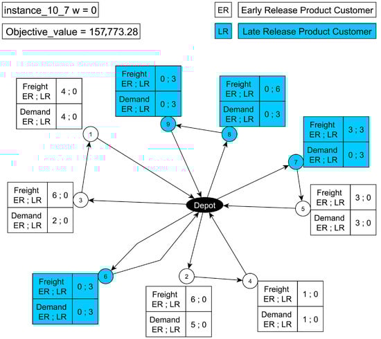
Figure 2. Traditional VRP (no reload), instance_10_7.

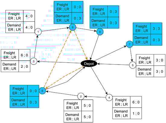
Figure 3. Proposed model with reload, instance_10_7.

The following analysis is based on the results obtained, shown in Table 2, Table 3, Table 4 and Table 5, which pertain to the Relative Gap, the computational time (in seconds, CPU s), and the efficiency (Ef), expressed as time (s) per node explored in the branch-and-bound ($B\&B$) search, multiplied by ${10}^4$, by model (MILP-3 and MILP-2) and by instance size (N).

Table 2. Analysis of computational results Instance N = 10.

	MILP-2					MILP-3
Instance	Objective Value	Best Bound	CPU (s)	Relative Gap	Ef	Objective Value	Best Bound	CPU (s)	Relative Gap	Ef
10_0	107,847.24	107,847.24	0.28	0.00%	3.94	107,847.24	107,847.24	3.54	0.00%	4.60
10_1	128,668.62	128,668.62	0.47	0.00%	6.41	128,668.62	128,668.62	11.00	0.00%	4.12
10_2	141,662.08	141,662.08	0.41	0.00%	1.55	141,662.08	141,662.08	94.53	0.00%	7.09
10_3	131,745.42	131,745.42	0.32	0.00%	1.97	131,745.42	131,745.42	11.85	0.00%	9.90
10_4	143,910.84	143,910.84	3.31	0.00%	1.43	143,910.84	143,910.84	124.85	0.00%	4.92
10_5	84,885.96	84,885.96	0.24	0.00%	3.93	84,885.96	84,885.96	0.65	0.00%	3.49
10_6	94,354.90	94,354.90	0.29	0.00%	5.15	94,354.90	94,354.90	0.50	0.00%	2.85
10_7	146,313.14	146,313.14	8.58	0.00%	1.44	146,313.14	146,313.14	2420.57	0.00%	5.44
10_8	181,688.34	181,688.34	0.50	0.00%	1.43	181,688.34	181,688.34	90.60	0.00%	6.97
10_9	135,284.02	135,284.02	0.31	0.00%	1.13	135,284.02	135,284.02	3.38	0.00%	3.11

Table 3. Analysis of computational results instance N = 15.

	MILP-2					MILP-3
Instance	Objective Value	Best Bound	CPU (s)	Relative Gap	Ef	Objective Value	Best Bound	CPU (s)	Relative Gap	Ef
15_0	178,631.62	178,631.62	955.12	0.00%	4.06	181,343.54	120,750.79	3600.00	33.41%	9.51
15_1	147,447.00	147,447.00	10.70	0.00%	4.05	147,446.99	130,713.82	3600.02	11.35%	33.13
15_2	135,517.23	129,513.59	3600.00	4.43%	5.47	137,009.06	88,879.03	3600.02	35.13%	18.73
15_3	149,502.96	130,724.18	3600.00	12.56%	2.68	149,502.96	105,187.63	3600.00	29.64%	14.30
15_4	145,325.80	145,325.80	2297.69	0.00%	3.63	145,325.82	107,827.68	3600.01	25.80%	21.64
15_5	159,148.10	159,148.10	9.07	0.00%	4.02	159,148.10	119,917.96	3600.01	24.65%	33.58
15_6	186,483.06	186,483.06	22.64	0.00%	3.92	186,483.06	152,015.60	3600.02	18.48%	45.83
15_7	179,994.24	179,994.24	1419.13	0.00%	4.35	179,994.24	124,638.66	3600.01	30.75%	18.80
15_8	176,316.78	176,316.78	265.67	0.00%	3.27	179,247.32	138,258.97	3600.01	22.87%	14.51
15_9	167,197.14	167,197.14	62.13	0.00%	3.19	167,197.14	135,033.02	3600.01	19.24%	18.86

Table 4. Analysis of computational results Instance N = 20.

	MILP-2					MILP-3
Instance	Objective Value	Best Bound	CPU (s)	Relative Gap	Ef	Objective Value	Best Bound	CPU (s)	Relative Gap	Ef
20_0	239,160.56	239,139.89	1715.85	0.00%	8.86	240,946.02	139,164.12	3600.01	42.24%	18.74
20_1	211,358.56	181,571.15	3600.00	14.09%	6.69	215,540.30	126,090.73	3600.01	41.50%	18.00
20_2	172,203.41	172,203.41	3432.54	0.00%	7.42	173,735.78	111,185.35	3600.03	36.00%	88.96
20_3	232,695.73	174,208.35	3600.01	25.13%	8.76	238,922.20	101,468.01	3600.01	57.53%	45.80
20_4	189,382.08	167,021.26	3600.00	11.81%	10.12	206,518.38	122,864.44	3600.01	40.51%	53.58
20_5	202,338.14	174,009.48	3600.00	14.00%	8.33	197,597.70	122,877.04	3600.01	37.81%	23.12
20_6	192,692.28	153,943.86	3600.01	20.11%	8.43	199,772.78	118,777.13	3600.03	40.54%	32.34
20_7	261,591.00	237,461.96	3600.01	9.22%	8.49	265,056.60	173,350.43	3600.01	34.60%	24.95
20_8	184,828.21	158,246.41	3600.00	14.38%	8.85	185,345.62	93,097.90	3600.02	49.77%	52.10
20_9	224,869.34	196,671.83	3600.00	12.54%	7.09	229,875.42	126,535.69	3600.01	44.95%	20.77

Table 5. Analysis of computational results instance N = 25.

	MILP-2					MILP-3
Instance	Objective Value	Best Bound	CPU (s)	Relative Gap	Ef	Objective Value	Best Bound	CPU (s)	Relative Gap	Ef
25_0	256,587.42	174,463.48	3600.00	32.01%	8.47	269,513.80	112,222.05	3600.04	58.36%	23.99
25_1	265,842.89	218,669.80	3600.01	17.74%	13.91	269,041.20	112,715.27	3600.01	58.10%	38.44
25_2	220,234.34	179,000.34	3600.01	18.72%	9.74	235,070.72	112,761.82	3600.02	52.03%	26.04
25_3	298,452.78	212,708.83	3600.00	28.73%	11.27	305,607.50	145,382.67	3600.02	52.43%	51.03
25_4	204,914.88	141,279.89	3600.00	31.05%	9.88	211,211.88	87,465.78	3600.01	58.59%	24.49
25_5	264,082.98	137,642.25	3600.01	47.88%	11.01	285,276.14	88,400.18	3600.01	69.01%	24.49
25_6	346,155.68	227,715.12	3600.01	34.22%	8.54	-	-	-	-	-
25_7	239,082.58	178,997.61	3600.01	25.13%	13.04	242,536.24	115,110.88	3600.01	52.54%	27.35
25_8	268,228.52	201,062.98	3600.01	25.04%	17.70	273,273.80	128,698.12	3600.01	52.91%	61.64
25_9	255,763.96	185,736.29	3600.00	27.38%	10.19	278,945.30	134,119.43	3600.02	51.92%	27.65

“-” indicates that no feasible solution was reported within the time limit.

• Relative Gap.
  For $N=10$, MILP-3 reaches optimality in all instances; in contrast, for $N=15$ it returns only feasible solutions, with gaps between 11.35% and 35.13%. For $N=20$ it likewise yields only feasible solutions, with an average gap of 42.54%; the same holds for $N=25$, with an average gap of 56.20%, and it fails to find a feasible solution for 25_6.
  For MILP-2, at $N=10$ it matches MILP-3 (optimal in all instances), but it outperforms it as N increases: at $N=15$ it attains optimality in $8/10$ instances and, for those that hit the time limit 15_2 and 15_3, it returns feasible solutions with gaps of $4.43\%$ and $12.56\%$. For $N=20$ it is optimal in $2/10$ instances and reports an average gap of $12.12\%$; at $N=25$ it yields only feasible solutions with an average gap of $28.79\%$.
• Computational Time (CPU (s)).
  For $N=10$, MILP-3 records an average time of $276.15\mathrm{s}$ and a maximum of $2420.57\mathrm{s}$ (in 10_7). For $N=15$, it reaches the time limit in all instances, as it does for $N=20$ and $N=25$. It is also shown that in 25_6 MILP-3 does not report a feasible solution.
  For MILP-2 $N=10$, the average solution time is $1.47\mathrm{s}$, with a maximum of $8.58\mathrm{s}$ in 10_7. At $N=15$, the solution time averages $1224.22\mathrm{s}$ and it reaches the limit only in 15_2 and 15_3. For $N=20$, MILP-2 reaches optimal status in 2 out of 10 instances 20_0 and 20_2, whereas for $N=25$, as with MILP-3, it reaches the time limit. Overall, the results show that MILP-2 shows greater efficiency.
• Efficiency $(Ef={10}^4\ast CPU\left(\mathrm{s}\right)/Nodes(B\&B))$.
  For $N=10$, MILP-3 records an average $Ef$ of $5.25$ and a maximum of $9.90$ (in 10_3). For $N=15$, the average is $22.89$ and the maximum $45.83$ (in 15_6). For larger instances, such as $N=20$, the average reaches $37.84$ with a maximum of $88.96$ (in 20_2), and for $N=25$ the average is $33.90$ with a maximum of $61.64$ (in 25_8). Note that in 25_6 no feasible solution is reported, and it is not included in the average.
  Now, for MILP-2, at $N=10$ the average $Ef$ is $2.84$ with a maximum of $6.41$ (in 10_1). At $N=15$, the average is $3.86$ and the maximum $5.47$ (in 15_2). For $N=20$, the average is $8.30$ with a maximum of $10.12$ (in 20_4). For $N=25$, the average is $11.38$ with a maximum of $17.70$ (in 25_8). Overall, the results indicate that the average $Ef$ value of MILP-2 is lower than that of MILP-3 by factors of approximately 1.85, 5.92, 4.56, and 2.98 for instance sizes $N=10$, 15, 20, and 25, respectively, which demonstrates the superior computational efficiency of MILP-2.

5.3. Fleet Usage and Reloading Analysis

The following analysis is based on the obtained results, shown in Table 6, Table 7, Table 8 and Table 9, which concern the Available Fleet (K) vs. Used Fleet ($K^{*}$) and Reload Satellites (w) vs. Route Reloading (r), by instance size (N) and by model (MILP-3 and MILP-2).

Table 6. Fleet usage and reloading analysis by model and instance size N = 10.

	MILP-2				MILP-3
Instance	$\mathbf{K}$	${\mathbf{K}}^{*}$	$\mathbf{w}$	$\mathbf{r}$	$\mathbf{K}$	${\mathbf{K}}^{*}$	$\mathbf{w}$	$\mathbf{r}$
10_0	4	4	0	0	4	4	0	0
10_1	5	3	2	2	5	3	2	2
10_2	6	4	2	2	6	4	2	2
10_3	8	4	4	3	8	4	4	2
10_4	5	3	1	1	5	3	1	1
10_5	3	3	0	0	3	3	0	0
10_6	3	3	0	0	3	3	0	0
10_7	5	3	2	2	5	3	1	1
10_8	5	4	2	2	5	4	2	2
10_9	4	4	1	1	4	4	1	1

Table 7. Fleet usage and reloading analysis by model and instance size N = 15.

	MILP-2				MILP-3
Instance	$\mathbf{K}$	${\mathbf{K}}^{*}$	$\mathbf{w}$	$\mathbf{r}$	$\mathbf{K}$	${\mathbf{K}}^{*}$	$\mathbf{w}$	$\mathbf{r}$
15_0	7	4	3	2	7	4	3	2
15_1	8	4	5	3	8	4	5	3
15_2	7	3	5	3	7	3	5	3
15_3	7	3	3	3	7	3	3	3
15_4	8	3	4	3	8	3	5	3
15_5	8	6	3	3	8	6	3	3
15_6	8	5	6	5	8	5	4	4
15_7	6	5	2	1	6	5	2	1
15_8	7	5	2	2	7	4	2	2
15_9	6	4	2	1	6	4	3	1

Table 8. Fleet usage and reloading analysis by model and instance size N = 20.

	MILP-2				MILP-3
Instance	$\mathbf{K}$	${\mathbf{K}}^{*}$	$\mathbf{w}$	$\mathbf{r}$	$\mathbf{K}$	${\mathbf{K}}^{*}$	$\mathbf{w}$	$\mathbf{r}$
20_0	10	7	4	3	10	7	4	3
20_1	8	7	3	2	8	8	1	1
20_2	9	6	3	1	9	8	0	0
20_3	9	6	3	2	9	6	2	2
20_4	8	5	4	3	8	6	2	2
20_5	11	5	6	3	11	4	6	3
20_6	9	5	4	4	9	5	4	4
20_7	10	8	5	4	10	7	4	3
20_8	9	6	6	5	9	6	5	3
20_9	8	6	3	3	8	6	3	3

Table 9. Fleet usage and reloading analysis by model and instance size N = 25.

	MILP-2				MILP-3
Instance	$\mathbf{K}$	${\mathbf{K}}^{*}$	$\mathbf{w}$	$\mathbf{r}$	$\mathbf{K}$	${\mathbf{K}}^{*}$	$\mathbf{w}$	$\mathbf{r}$
25_0	10	6	4	4	10	7	3	3
25_1	11	9	4	4	11	9	2	2
25_2	11	8	4	3	11	8	3	3
25_3	12	8	6	4	12	8	4	4
25_4	11	6	6	4	11	7	5	4
25_5	10	7	3	3	10	7	4	3
25_6	10	8	3	3	–	–	–	–
25_7	11	7	6	3	11	6	4	4
25_8	12	7	7	6	12	8	6	6
25_9	9	6	5	3	9	7	4	3

K: available fleet; K*: used fleet; w: reload satellites; r: routes with reload. − indicates that no feasible solution was reported within the time limit.

• Available Fleet (K) vs. Used Fleet $K^{*}$.
  MILP-3 shows a used fleet $K^{*}$ between 3 and 4, with an average of 1–2 idle vehicles and a maximum of 4 (10_3) for $N=10$, where the status is optimal in all 10 instances (see Table 6). For $N=15$ (Table 7), where feasible solutions are obtained in all ten instances, the used fleet lies between $K^{*}=3$ and 6, with between 1 and 5 idle delivery vehicles (maximum in 15_4). As shown in Table 8, for $N=20$, feasible solutions indicate $K^{*}$ between 4 and 8, with up to 7 idle vehicles, as in 20_5. For $N=25$ (As shown in Table 9), feasible solutions indicate that in $9/10$ instances (no feasible solution in 25_6), the model uses between $K^{*}=6$ and 9 delivery vehicles, with between 2 and 5 idle vehicles (maximum idle capacity in 25_7).
  For MILP-2, in the $N=10$ instances, availability K ranges from 3 to 8, the used fleet $K^{*}$ is between 3 and 4, with a maximum of 4 idle vehicles in 10_3. All delivery vehicles are used in $4/10$ instances (10_0, 10_5, 10_6, 10_9). For $N=15$, K ranges from 6 to 8, $K^{*}$ from 3 to 6, and idle vehicles range from a minimum of 1 to a maximum of 5 (maximum in 15_4) (see Table 6 and Table 7).
  As shown in Table 8 and Table 9, for $N=20$ and $N=25$, available K ranges from 8–11 and 9–12, respectively. For $N=20$, $K^{*}$ lies between 5 and 8, with a maximum of 6 idle vehicles (in 20_5); for $N=25$, $K^{*}$ is between 6 and 9, with a maximum of 5 idle vehicles in 25_4 and 25_8.
• Reload Satellites (w) vs. Route Reloading (r).
  For the use of reload satellites (w) and route reloading (r), in MILP-3 satellites are used in $7/10$ instances for $N=10$. 10_3 stands out with $w=4$ and only $r=2$, hence $w-r=2$, implying that at least one route was reloaded more than once. For the same instance in MILP-2, $w-r=1$, which also indicates that at least one route is reloaded more than once. Note that MILP-2 reaches the same solutions as MILP-3 except for the aforementioned instance and for 10_7, where MILP-3 has $w=1$ whereas MILP-2 has $w=2$ (Table 6).
  For MILP-3 with $N=15$, the average w lies between 3 and 4, while per instance between $r=1$ and 4 routes are reloaded. 15_1 and 15_2 stand out (each with $r=3$ and $w=5$) as well as 15_9 ($w=3$, $r=1$). In these cases $w>r$, indicating multiple reloads on at least one route. For MILP-2, w ranges from 2 to 6, while r ranges from 1 to 5. There is $w>r$ in $7/10$ instances (15_0, 15_1, 15_2, 15_4, 15_6, 15_7, 15_9) and $w=r$ in $3/10$ (15_3, 15_5, 15_8). The maximum difference is $w-r=2$ in 15_1 and 15_2 (Table 7).
  For $N=20$, in MILP-3 the average w lies between 3 and 4; 20_5 stands out with $w=6$ over $r=3$ routes ($w-r=3$), implying multiple reloads on at least one route. For MILP-2, w ranges from 3 to 6 and r from 1 to 5. We have $w>r$ in $8/10$ cases (20_0, 20_1, 20_2, 20_3, 20_4, 20_5, 20_7, 20_8) and $w=r$ in $2/10$ (20_6, 20_9). The maximum difference is $w-r=3$ in 20_5 (Table 8).
  With $N=25$, in MILP-3 25_4, 25_5, and 25_9 stand out, where more satellites than routes are used ($w>r$), hence $w-r>0$, indicating that at least one route is reloaded more than once. In contrast, for MILP-2, w ranges from 3 to 7 with r between 3 and 6; there is $w>r$ in $6/10$ instances (25_2, 25_3, 25_4, 25_7, 25_8, 25_9) and $w=r$ in $4/10$ (25_0, 25_1, 25_5, 25_6), with a maximum difference of $w-r=3$ in 25_7 (Table 9).
  As shown in Table 10 and Table 11, both models exhibit exponential growth in computation time as the number of nodes increases, which is consistent with the NP-hard nature of the vehicle routing problem. Nevertheless, the MILP-2 formulation demonstrates better scalability than MILP-3. This can be observed in the data from the tables, where the number of variables and constraints in MILP-2 depends only on the number of nodes and remains constant for a given instance size, whereas in MILP-3 these values increase with the number of vehicles. The inclusion of the vehicle index k in MILP-3 results in a larger model, negatively impacting its computational performance. Consequently, MILP-2 can handle larger fleets without increasing computation time, thus achieving greater efficiency and scalability.
  Table 10. Analysis of number of variables and constraints for the MILP-2 formulation ($K=1$–10).

  	K = 1–10
  Instance	Var	Constr
  10	247	512
  15	522	1072
  20	897	1832
  25	1372	2792
  50	5247	10,592
  75	11,622	23,392
  100	20,497	41,192

  Table 11. Analysis of number of variables and constraints for the MILP-3 formulation (split by $K=1$–5 and $K=6$–10).

  Instance	K Range	Var’s	Constr’s	Var’s	Constr’s	Var’s	Constr’s	Var’s	Constr’s	Var’s	Constr’s
  10	1–5	231	522	362	887	493	1252	624	1617	755	1982
  	6–10	886	2347	1017	2712	1148	3077	1279	3442	1410	3807
  15	1–5	496	1087	767	1862	1038	2637	1309	3412	1580	4187
  	6–10	1851	4962	2122	5737	2393	6512	2664	7287	2935	8062
  20	1–5	861	1852	1322	3187	1783	4522	2244	5857	2705	7192
  	6–10	3166	8527	3627	9862	4088	11,197	4549	12,532	5010	13,867
  25	1–5	1326	2817	2027	4862	2728	6907	3429	8952	4130	10,997
  	6–10	4831	13,042	5532	15,087	6233	17,132	6934	19,177	7635	21,222
  50	1–5	5151	10,642	7802	18,487	10,453	26,332	13,104	34,177	15,755	42,022
  	6–10	18,406	49,867	21,057	57,712	23,708	65,557	26,359	73,402	29,010	81,247
  75	1–5	11,476	23,467	17,327	40,862	23,178	58,257	29,029	75,652	34,880	93,047
  	6–10	40,731	110,442	46,582	127,837	52,433	145,232	58,284	162,627	64,135	180,022
  100	1–5	20,301	41,292	30,602	71,987	40,903	102,682	51,204	133,377	61,505	164,072
  	6–10	71,806	194,767	82,107	225,462	92,408	256,157	102,709	286,852	113,010	317,547

• Results of the Proposed VRP-RT-RMS Model.
  Figure 4 shows the model solution for instance 15_1. The dashed line indicates the tour of the reload vehicle, which follows the route [0, 12, 9, 11, 14, 8, 0] as depicted. Reloads occur across different delivery routes and, in particular, multiple reloads within a single route (Node_12, Node_15, Node_9). This behavior is consistent with the vehicle capacity ($Q_v=6$) and with the cumulative demand, which exceeds what can be carried in a single trip; therefore, the delivery vehicle must be assisted several times by the reload tour.
  

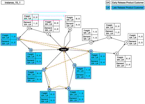  Figure 4. Solution for instance_15_1.
  Figure 5 presents the model behavior for instance 15_6. The reload vehicle tour according to the table is [0, 3, 1, 5, 14, 12, 2, 0]. In this solution, the same delivery vehicle is reloaded twice along its route, but not at consecutive nodes. This occurs on route [0, 5, 13, 7, 12, 0]: the reloads take place at nodes 5 and 12, with two intermediate visits (13 and 7). This pattern is consistent with the delivery vehicle capacity ($Q_v=5$) and with the cumulative demand and product mix, which require reloading at different points of the tour. The reload vehicle serves multiple delivery routes; between the two reloads of the same route (at 5 and 12), it reloads another vehicle at node 14 before returning to complete the second reload.
  

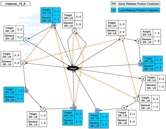  Figure 5. Solution for instance_15_6.

6. Conclusions

This work introduces VRP-RT-RMS, a variant that jointly integrates late product availability, enabling delivery through en-route reload of the delivery vehicles via a reload vehicle that operates at satellites located at customer nodes. The formulation captures key last-mile decisions, such as satellite selection, synchronization between the delivery vehicle and the reload vehicle, compliance with release times, and conservation of load by non-interchangeable product type. To solve the problem, two Mixed-Integer Linear Programming (MILP) models are proposed: one with three indices (MILP-3) and another with two indices (MILP-2). In the former, the decision variables include the subscript k, which represents the delivery vehicle performing the route and belongs to the set $Kp$, corresponding to the number of available delivery vehicles. In contrast, in the MILP-2 model, this subscript is omitted from the decision variables, and the set $Kp$ is treated as a parameter. The experimental results show that both formulations optimally solve small instances; however, as the problem size increases, MILP-2 exhibits better performance in CPU time and efficiency per explored node, maintaining substantially smaller optimality gaps when the time limit is reached.

When comparing our results with the exact optimization reported by [15], who solved small-size instances (8–14 nodes), it is observed that the proposed VRP-RT-RMS model, which integrates release times, in-route reloading, and vehicle synchronization, presents greater computational complexity. Despite this additional difficulty, the exact MILP-2 formulation achieves optimal solutions for instances up to 15 nodes and feasible solutions for instances up to 25 nodes, demonstrating better performance and representing a significant advancement in the exact optimization of routing problems with synchronization and release constraints.

Similarly, other exact approaches in the literature show comparable computational limitations: [26] solved only 12 small-scale instances (15–60 nodes) within a two-hour limit; [25] reached optimality only for cases with up to 16 trucks; and [23] applied a bi-objective exact method to the Collaborative Feeder VRP, which was computationally feasible only for small instances of 8–12 nodes.

In terms of solution improvement, enabling en-route reload simultaneously reduces the total cost and the effectively used fleet compared with a traditional VRP without reload. It is also observed that, in specific scenarios, the reload-enabled VRP finds feasible solutions that are infeasible under the traditional VRP because of vehicle capacity. Another observed phenomenon is that the number of satellites visited exceeds the number of reloaded routes, which shows the value of allowing multiple reloads on the same route when the demand mix and the vehicle capacity so require.

As a methodological takeaway, we conclude that MILP-3 is useful as a reference model to understand the problem’s behavior and to validate synchronization, but its efficiency degrades as instance size increases. In contrast, MILP-2 attains lower optimality gaps and higher efficiency on the same instances, offering a better accuracy–scalability trade-off. Therefore, it is the preferred option for sensitivity analyses. In addition, the strategy of mobile satellites with post-release reloading yields better results in last-mile logistics: it reduces total distance and fleet usage, and can restore feasibility when the classical VRP is infeasible.

In addition to these findings, from a methodological perspective, this study focused on optimizing a single objective aimed at minimizing the total traveled distance as a representative measure of operational cost. The model effectively achieved a reduction in the total travel distance, thereby lowering overall operating costs, as well as reducing the number of delivery vehicles used. However, we acknowledge that this single-objective approach may limit the scope of the analysis by not considering other relevant criteria in logistics decision-making or allowing a more in-depth evaluation of these variables. Recent studies, such as [31], have proposed multi-objective formulations that jointly address economic, social, and operational aspects. In this sense, a future research direction consists of extending the VRP-RT-RMS model toward a multi-objective framework that balances different logistics performance criteria.

As future research directions, we propose the incorporation of metaheuristic techniques to find feasible solutions in larger instances, since, as shown in the largest experiment ($N=25$), MILP-2 reached a $47.87\%$ gap within the 3600-s limit. Other promising extensions include the integration of stochastic demand or stochastic release times.

From an operational perspective, the VRP-RT-RMS model serves as a valuable tool for planning and decision making in last-mile distribution operations with late product availability. The ability to perform en-route reloading at mobile satellite points reduces vehicle idle time, decreases the required fleet size, and avoids unnecessary returns to the depot, thereby maintaining service continuity. These operational improvements translate directly into economic savings by lowering travel times and distances, minimizing the need to dispatch additional vehicles for late-release products, and reducing the overall number of vehicles required to complete deliveries.

Furthermore, the model provides useful insights for the temporal coordination between different types of vehicles, supporting the definition of more efficient release windows and synchronization strategies between delivery and reloading vehicles. These strategies enhance operational efficiency.

From a managerial standpoint, the results can guide the development of logistics policies aimed at optimizing resource utilization, improving energy efficiency and increasing operational flexibility in response to variations in product availability or daily demand.

References

- Salehi Sarbijan, M.; Behnamian, J. Emerging research fields in vehicle routing problem: A short review. Arch. Comput. Methods Eng. 2023, 30, 2473–2491. [Google Scholar] [CrossRef]
- Lo, S.C.; Chuang, Y.L. Vehicle routing optimization with cross-docking based on an artificial immune system in logistics management. Mathematics 2023, 11, 811. [Google Scholar] [CrossRef]
- Yu, V.F.; Lin, C.H.; Maglasang, R.S.; Lin, S.W.; Chen, K.F. An Efficient Simulated Annealing Algorithm for the Vehicle Routing Problem in Omnichannel Distribution. Mathematics 2024, 12, 3664. [Google Scholar] [CrossRef]
- Mardešić, N.; Erdelić, T.; Carić, T.; Đurasević, M. Review of stochastic dynamic vehicle routing in the evolving urban logistics environment. Mathematics 2023, 12, 28. [Google Scholar] [CrossRef]
- Ambrosino, D.; Cerrone, C. A Rich Vehicle Routing Problem for a City Logistics Problem. Mathematics 2022, 10, 191. [Google Scholar] [CrossRef]
- Huang, Y.H.; Blazquez, C.A.; Huang, S.H.; Paredes-Belmar, G.; Latorre-Nuñez, G. Solving the feeder vehicle routing problem using ant colony optimization. Comput. Ind. Eng. 2019, 127, 520–535. [Google Scholar] [CrossRef]
- Pillac, V.; Gendreau, M.; Guéret, C.; Medaglia, A.L. A review of dynamic vehicle routing problems. Eur. J. Oper. Res. 2013, 225, 1–11. [Google Scholar] [CrossRef]
- Cruijssen, F.; Bräysy, O.; Dullaert, W.; Fleuren, H.; Salomon, M. Joint route planning under varying market conditions. Int. J. Phys. Distrib. Logist. Manag. 2007, 37, 287–304. [Google Scholar] [CrossRef]
- Yousefikhoshbakht, M.; Chaharmahali, M.; Ahmed, Z.H. The Line-Haul Feeder Vehicle Routing Problem: A Classification and Review. Complexity 2023, 2023, 9902545. [Google Scholar] [CrossRef]
- Torres-Tapia, W.; Montoya-Torres, J.; Ruiz-Meza, J. Hybrid ils-vnd algorithm for the vehicle routing problem with release times. In Applied Computer Sciences in Engineering; Springer: Cham, Switzerland, 2022; pp. 222–233. [Google Scholar] [CrossRef]
- Bard, J.F.; Huang, L.; Jaillet, P.; Dror, M. A decomposition approach to the inventory routing problem with satellite facilities. Transp. Sci. 1998, 32, 189–203. [Google Scholar] [CrossRef]
- Lan, Y.L.; Liu, F.G.; Huang, Z.; Ng, W.W.; Zhong, J. Two-echelon dispatching problem with mobile satellites in city logistics. IEEE Trans. Intell. Transp. Syst. 2020, 23, 84–96. [Google Scholar] [CrossRef]
- Ancele, Y.; Hà, M.H.; Lersteau, C.; Matellini, D.B.; Nguyen, T.T. Toward a more flexible VRP with pickup and delivery allowing consolidations. Transp. Res. Part C Emerg. Technol. 2021, 128, 103077. [Google Scholar] [CrossRef]
- Soto-Concha, R.; Escobar, J.W.; Morillo-Torres, D.; Linfati, R. The Vehicle-Routing Problem with Satellites Utilization: A Systematic Review of the Literature. Mathematics 2025, 13, 1092. [Google Scholar] [CrossRef]
- Sarbijan, M.S.; Behnamian, J. Multi-fleet feeder vehicle routing problem using hybrid metaheuristic. Comput. Oper. Res. 2022, 141, 105696. [Google Scholar] [CrossRef]
- Chen, H.K.; Chou, H.W.; Hsueh, C.F.; Ho, T.Y. The linehaul-feeder vehicle routing problem with virtual depots. IEEE Trans. Autom. Sci. Eng. 2011, 8, 694–704. [Google Scholar] [CrossRef]
- Chen, H.K.; Chou, H.W.; Hsu, C.Y. The Linehaul-Feeder Vehicle Routing Problem with Virtual Depots and Time Windows. Math. Probl. Eng. 2011, 2011, 759418. [Google Scholar] [CrossRef]
- Brandstätter, C.; Reimann, M. The line-haul feeder vehicle routing problem: Mathematical model formulation and heuristic approaches. Eur. J. Oper. Res. 2018, 270, 157–170. [Google Scholar] [CrossRef]
- Brandstätter, C. A metaheuristic algorithm and structured analysis for the line-haul feeder vehicle routing problem with time windows. Cent. Eur. J. Oper. Res. 2021, 29, 247–289. [Google Scholar] [CrossRef]
- Chen, H.K.; Wang, H. A two-stage algorithm for the extended linehaul-feeder vehicle routing problem with time windows. Int. J. Shipp. Transp. Logist. 2012, 4, 339–356. [Google Scholar] [CrossRef]
- Sarbijan, M.S.; Behnamian, J. A mathematical model and metaheuristic approach to solve the real-time feeder vehicle routing problem. Comput. Ind. Eng. 2023, 185, 109684. [Google Scholar] [CrossRef]
- Sarbijan, M.S.; Behnamian, J. Real-time collaborative feeder vehicle routing problem with flexible time windows. Swarm Evol. Comput. 2022, 75, 101201. [Google Scholar] [CrossRef]
- Salehi Sarbijan, M.; Behnamian, J. Feeder vehicle routing problem in a collaborative environment using hybrid particle swarm optimization and adaptive learning strategy. Environ. Dev. Sustain. 2023, 27, 6165–6205. [Google Scholar] [CrossRef]
- Bevilaqua, A.; Bevilaqua, D.; Yamanaka, K. Parallel island based Memetic Algorithm with Lin–Kernighan local search for a real-life Two-Echelon Heterogeneous Vehicle Routing Problem based on Brazilian wholesale companies. Appl. Soft Comput. 2019, 76, 697–711. [Google Scholar] [CrossRef]
- Maknoon, M.; Kone, O.; Baptiste, P. A sequential priority-based heuristic for scheduling material handling in a satellite cross-dock. Comput. Ind. Eng. 2014, 72, 43–49. [Google Scholar] [CrossRef]
- Li, H.; Zhang, L.; Lv, T.; Chang, X. The two-echelon time-constrained vehicle routing problem in linehaul-delivery systems. Transp. Res. Part B Methodol. 2016, 94, 169–188. [Google Scholar] [CrossRef]
- Mühlbauer, F.; Fontaine, P. A parallelised large neighbourhood search heuristic for the asymmetric two-echelon vehicle routing problem with swap containers for cargo-bicycles. Eur. J. Oper. Res. 2021, 289, 742–757. [Google Scholar] [CrossRef]
- Yang, J.; Wang, J. A Hybrid Method Combing Reinforcement Learning and Heuristics in Solving Two-Echelon Vehicle Routing Problem with Backhauls. In Knowledge Science, Engineering and Management; Springer: Singapore, 2024; pp. 241–253. [Google Scholar] [CrossRef]
- Babagolzadeh, M.; Zhang, Y.; Abbasi, B.; Shrestha, A.; Zhang, A. Promoting Australian regional airports with subsidy schemes: Optimised downstream logistics using vehicle routing problem. Transp. Policy 2022, 128, 38–51. [Google Scholar] [CrossRef]
- Xue, G.; Wang, Z. Order acceptance and scheduling in the instant delivery system. Comput. Ind. Eng. 2023, 182, 109395. [Google Scholar] [CrossRef]
- Ransikarbum, K.; Wattanasaeng, N.; Madathil, S.C. Analysis of multi-objective vehicle routing problem with flexible time windows: The implication for open innovation dynamics. J. Open Innov. Technol. Mark. Complex. 2023, 9, 100024. [Google Scholar] [CrossRef]
Disclaimer/Publisher’s Note: The statements, opinions and data contained in all publications are solely those of the individual author(s) and contributor(s) and not of MDPI and/or the editor(s). MDPI and/or the editor(s) disclaim responsibility for any injury to people or property resulting from any ideas, methods, instructions or products referred to in the content. |
© 2025 by the authors. Licensee MDPI, Basel, Switzerland. This article is an open access article distributed under the terms and conditions of the Creative Commons Attribution (CC BY) license (https://creativecommons.org/licenses/by/4.0/).