Abstract
Replicating runs in designed experiments is essential for unbiased error variance estimation, particularly when the fitted model may not account for all active effects. Definitive screening designs (DSDs), while offering orthogonality between main effects and quadratic terms, face critical limitations in error estimation when fitting the full quadratic model. For even numbers of factors (6, 8, 10, 12), the basic DSD provides zero degrees of freedom for error variance estimation, while odd-factor designs (5, 7, 9, 11) retain only two degrees of freedom, both insufficient for reliable statistical inference. This study presents a comprehensive investigation of partial replication strategies for DSDs with even factors (6, 8, 10, 12) and odd factors (5, 7, 9, 11), examining the addition of two, four, six, and eight replicated runs under two distinct configurations: balanced replication (Case 1) and unbalanced replication (Case 2). We systematically evaluate the trade-offs between statistical power, relative standard errors (RSEs), D-efficiency, and A-efficiency as functions of the replication level and number of factors. Our analysis demonstrates that replicating half the total runs achieves a high statistical power of 0.90–0.95 for main effects—retaining at least 90% of full replication’s power—while requiring only 62.5% of the experimental runs. The most significant improvement occurs after replicating four runs, where critical t-values decrease from 12.71 to 2.78, making effect detection practically feasible. The results show that balanced replication (Case 1) yields a lower RSE for quadratic effects, while unbalanced replication (Case 2) provides superior orthogonality with the maximum absolute correlations approaching zero. Comprehensive design matrices and performance metrics are provided in the appendices to ensure reproducibility. Based on empirical and theoretical considerations, we recommend half-partial replication as a highly efficient strategy that balances statistical rigor with resource constraints.
Keywords:
replication; pure error; power; relative standard error; definitive screening designs; second-order model MSC:
62K99
1. Introduction
Screening experiments [1] play a fundamental role in identifying active factors among many candidates with minimal experimental effort. Classical approaches include two-level fractional factorial designs [2,3] which efficiently screen main effects but require follow-up experiments to detect curvature. Definitive screening designs (DSDs) represent a more recent class of three-level designs, first introduced by [4].These designs involve m factors and comprise runs, notable for their orthogonality not only among the main effects but also between the main effects and the quadratic terms. Subsequently, Xiao et al. [5] extended the concept by constructing orthogonal DSDs using conference matrices, with the design matrix X structured as . Here, C denotes a conference matrix of order m, characterized by off-diagonal entries of and satisfying , with representing a zero vector of length m.
DSDs offer several advantageous properties that set them apart from other screening design methods, including alternative three-level approaches using weighing matrices [6]. However, despite these strengths, the efficiency estimation of quadratic terms can negatively impact statistical power and relative standard errors. DSDs are capable of accommodating models with an intercept, all main effects, and quadratic effects. Nonetheless, practitioners often limit their focus to either the main effects model or the model encompassing both main and quadratic effects. Utilizing the second-order model, which includes main effects and pure quadratic effects, leaves a limited number of degrees of freedom available for estimating the error variance. Consequently, this limitation results in a potentially imprecise variance estimate.
Incorporating replicated runs into DSDs effectively resolves these challenges by providing pure error degrees of freedom for precise error variance estimation. While the value of replication in DSDs is well established, a critical question remains unresolved: how much replication is necessary? The full replication of all design runs doubles the experimental cost, which may be prohibitive in resource-constrained settings. Conversely, minimal replication (such as adding only center points) provides insufficient degrees of freedom for robust inference. This creates a fundamental design dilemma: practitioners need guidance on partial replication strategies that achieve adequate statistical power while minimizing experimental burden. Despite the practical importance of this question, a systematic investigation of partial replication trade-offs for DSDs has not been undertaken in the literature. Additionally, the introduction of replicated runs enhances the design’s statistical power, particularly in the context of estimating the active effects.
While the foundational work on efficient designs with minimal aliasing [7] led to the development of DSDs [4], with Xiao et al. [5] establishing construction methods using conference matrices, subsequent research has explored various extensions including categorical factors [8] and fold-over designs [9], the specific question regarding efficient partial replication strategies remains incompletely addressed in the literature. Most existing work on DSDs has focused on construction methods [10], projection properties, blocking arrangements [11], model selection strategies, and data analysis techniques [12]. The practical question of how much replication is necessary to achieve adequate statistical power while minimizing experimental burden—a critical consideration for resource-constrained industrial experiments—has received limited systematic investigation. Recent work by the authors of [13] addresses the generation of optimal designs with user-specified pure replication structures, providing a general algorithmic framework for incorporating replication into experimental designs. Their coordinate-exchange algorithm can generate designs with arbitrary replication patterns, offering the maximum flexibility for customized scenarios. Our study complements this methodological framework by providing systematic empirical guidance specifically tailored to DSDs: we demonstrate, through comprehensive simulation across 5–12 factors, that half-partial replication (Definition 1, Section 3) achieves near-optimal power–efficiency balance—retaining at least 90% of full replication’s statistical power while requiring only 62.5% of experimental runs. This specificity enables practitioners to make informed replication decisions for standard DSD applications without requiring custom algorithmic optimization for each experimental scenario. While Walsh and Borkowski’s framework offers generality across design types, our targeted investigation provides ready-to-implement guidance for the common case of DSD screening experiments, including specific recommendations for balanced versus unbalanced replication strategies (Cases 1 and 2) and minimum replication thresholds. The specific application of partial replication strategies to DSDs and the systematic evaluation of power–efficiency trade-offs across a comprehensive range of practically relevant factor levels remain underexplored in the existing literature. This study addresses this gap by providing theoretical foundations and empirical guidance on partial replication that practitioners can readily implement across a range of factor levels commonly encountered in screening experiments.
Replication is firmly established as one of the foundational principles of experimental design, as highlighted by Fisher in [14,15], providing both model-independent error variance estimates and enhanced statistical power. These error variance estimates remain robust against the potential omissions of interaction effects, and the introduction of replicated runs enhances the design’s statistical power for detecting active effects.
This study addresses the following research questions: (1) What level of partial replication optimally balances statistical power for effect detection with experimental economy? (2) How do different replication strategies (balanced versus unbalanced) affect design performance? (3) At what replication level do diminishing returns emerge? We systematically investigate partial replication strategies involving two to eight additional runs for DSDs with even factors (6, 8, 10, 12) and odd factors (5, 7, 9, 11), evaluating trade-offs between statistical power, relative standard errors (RSEs), D-efficiency, and A-efficiency across this practically relevant range. Our theoretical and empirical analysis demonstrates that half-partial replication—replicating approximately half the total runs—achieves a statistical power of 0.90–0.95 for main effects, comparable to full replication, while requiring only 62.5% of the experimental runs. This finding establishes practical guidance for experimenters seeking to balance statistical rigor with resource constraints in screening experiments.
The evaluation of partial replication strategies employs D-efficiency and A-efficiency [16] as primary performance metrics. D-efficiency, which measures the determinant of the information matrix and is particularly well-suited for continuous factor designs, quantifies the precision of parameter estimation relative to an optimal design. Since DSDs utilize three-level continuous factors coded at −1, 0, and +1, D-efficiency provides an appropriate criterion for comparing design performance across different replication strategies. A-efficiency, based on the trace of the inverse information matrix, evaluates the average variance of parameter estimates and complements D-efficiency in assessing overall design quality.
A key research question concerns determining the optimal number of runs that should be replicated. It is essential to keep in mind that a more precise estimation of error variance is achieved with increased degrees of freedom. As demonstrated in Table 1, the critical value for testing the effects of DSDs at a significance level of varies significantly as the degrees of freedom increase from 1 to 13. With only one degree of freedom, an effect must be nearly 13 times its standard error to achieve significance. The following remarks formalizes this relationship: Replicating two runs notably reduces the critical value to 4.3, while replicating four runs further lowers it to 2.78. Beyond replicating four runs, the impact on the critical value diminishes.

Table 1.
Error degrees of freedom (d.f.) versus t critical value .
Additionally, the number of runs chosen for replication significantly influences the design’s statistical power to detect effects that hold practical significance. The practical significance of an effect can vary depending on the specific problem, but generally, effects of two standard deviations are considered substantial in many industrial scenarios. Attempting to control a process with smaller effects may not yield tangible improvements and could potentially adversely affect process capability.
Once the magnitude of significant effects is determined, the subsequent consideration revolves around defining the threshold for acceptable statistical power. The adequacy of statistical power can vary depending on the specific context. In our study, we advocate a target power range of to as it strikes a balance between achieving statistically robust results and minimizing the need for extensive experimentation. Consequently, our research delves into the impact of incorporating partially replicated runs on enhancing statistical power and reducing relative standard errors.
The following section will delve into the criteria for selecting appropriate experimental designs, shedding light on how the addition of various numbers of replicated runs to DSDs featuring even factors (6, 8, 10, 12) and odd factors (5, 7, 9, 11) influences these criteria. For a fundamental guide on executing and analyzing these designs, please refer to [17]. Additionally, we will present a methodology for making informed decisions regarding the selection of runs for replication, optimizing the overall design’s effectiveness.
2. Criteria for Choosing Between Designs
Statistics and experimental designs play a pivotal role in modeling collected data and providing insights into the parameters of interest. One fundamental model is the main effects model, expressed as follows:
Here, m signifies the number of factors, and the parameters stand as unknown constants denoting the intercept and main effects. The terms are independent and identically distributed random variables, following a normal distribution with a mean of 0 and a standard deviation of .
In our analysis, we expand upon this model to encompass both main effects and quadratic effects, referred to as the quadratic model:
In DSDs, two-factor interactions are partially aliased with quadratic effects due to the three-level structure, as documented by [4,5]. Following standard screening practice and the effect hierarchy principle [17], our study focuses on the main effects and quadratic model (Equation (2)), which is appropriate for identifying active factors and detecting curvature. Practitioners requiring interaction estimation would need fold-over or augmentation strategies [9]. Our replication strategy maintains this aliasing structure, acceptable for the screening context DSDs were designed for.
When to Consider Interaction Estimation: Several criteria should guide the decision to prioritize interaction estimation over the screening-focused main effects and quadratic model. Practitioners should consider interaction estimation when (1) strong prior knowledge or domain expertise suggests that specific two-factor interactions are likely to be active and practically significant; (2) the screening phase will be followed by optimization experiments specifically designed to investigate interactions among identified active factors; (3) preliminary analysis reveals significant lack-of-fit when fitting only main effects and quadratic terms, suggesting unmodeled interaction effects; or (4) the experimental context involves processes where synergistic or antagonistic factor relationships are theoretically expected. In such scenarios, fold-over designs [9] or augmentation strategies provide systematic approaches to de-aliasing interactions from quadratic effects. However, for initial screening experiments where the primary objective is identifying active factors and detecting curvature—the context for which DSDs were specifically designed—the main effects and quadratic model remains the appropriate and efficient choice.
For DSDs with m factors, the basic design contains runs. When fitting this quadratic model with parameters (intercept, m main effects, and m quadratic effects), the design becomes saturated or near-saturated, leaving zero or very few degrees of freedom for error variance estimation. This severe limitation in degrees of freedom makes reliable statistical inference impractical without replication—a fundamental motivation for this study.
A more concise notation employs vectors and matrices, illustrated as follows:
In this representation, y forms an vector of response values, X constitutes an matrix where p equals , represents a vector of unknown parameters to be estimated, and shapes an vector of errors, presumed to be independent and identically distributed with a mean of 0 and a standard deviation of .
The model matrix X is thoughtfully constructed to incorporate a column of ones for the intercept; m columns for the factor settings coded as ‘−1,’ ‘0,’ and ‘1;’ and an additional m columns dedicated to the quadratic terms. For example, in the context of a six-factor DSD, the quadratic model would necessitate a model matrix ‘X’ that comprises a column for the intercept, six columns for the main effects, and an additional six columns for the quadratic effects.
We will employ two well-known optimality criteria for experimental designs. The first criterion is the D-efficiency of a design and can be computed as follows:
Here, X represents the corresponding model matrix of the quadratic model. The maximization in the denominator extends over all possible designs, and p denotes the number of parameters in the model. For further insights into the D-efficiency criteria, please refer to [9,16,18]. The second criterion we will apply is the A-efficiency of the design, which can be calculated as follows:
Here, signifies the trace of X, which is the sum of its diagonal elements of X, and p again represents the number of parameters in the model. For further details regarding the A-efficiency criteria, please consult [9,16,18].
In addition to the efficiencies mentioned earlier, an experimenter should also consider the relative standard errors concerning the estimates of the model parameters in relation to the error standard deviation . In an ideal scenario, all relative standard errors would be equal, indicating that all effects are estimated with the same level of precision. In the context of DSDs, the relative standard error for all model parameter estimates, including both main and quadratic effects, is where n represents the number of runs in the design.
If it turns out that not all model parameters have uniform relative standard errors, it is beneficial for all parameters of a specific type to exhibit consistent relative standard errors. For instance, it is preferable for all main effects to have equivalent relative standard errors when there is no prior information available to discern which factors are more likely to be active. Similarly, for quadratic effects, it is advantageous for them all to possess the same relative standard error, as predicting in advance which (if any) will be active is uncertain. To prevent any favoritism towards certain effects, it is advantageous to ensure that all effects of a particular type have consistent variances.
3. Construction of Partially Replicated
This study focuses on DSDs with both an even and odd number of factors. Two specific cases are considered:
Case 1: In this scenario, the two selected runs exhibit the same pattern of zeroes and feature balanced columns, which means an equal number of plus and minus signs.
Case 2: In this case, the two selected runs do not exhibit the same pattern of zeroes, and thus the columns are unbalanced.
For an even number of factors, such as , it is possible to fit the intercept, all main effects, and all quadratic effects. However, this exhausts the degrees of freedom for estimating error variance. For instance, in a six-factor DSD, if only the basic 13-run design is used, and the goal is to fit the quadratic model, the statistical power to detect the effects of two standard deviations is only for main effects, for quadratic effects, and for the intercept.
For an odd number of factors, like , it is possible to fit the intercept, all main effects, and all quadratic effects while retaining two degrees of freedom for estimating error variance. The construction of DSDs with an odd number of factors, introduced by [5], involves starting with a DSD of even factors and removing one column. For example, in the case of five factors, the DSD is constructed from the six-factor DSD by removing one column. With the basic 13-run design, the statistical power to detect the effects of two standard deviations is for main effects, for quadratic effects, and for the intercept.
When an even design is fully replicated, the power increases to for main effects, for quadratic effects, and for the intercept. Similarly, when an odd design is replicated twice, the power increases to for main effects, for quadratic effects, and for the intercept. Both even and odd designs require a total of 25 runs, i.e., double the 12 runs needed for the DSD of six factors (or five factors by deleting one column), plus one center point. This leads to a crucial question: what can be achieved with fewer runs?
3.1. Statistical Foundation and Replication Strategy
To address this question systematically, we first review the well-established statistical principles governing replication and then develop our partial replication strategy. The relationship between degrees of freedom from replication and hypothesis testing capability is fundamental to experimental design.
Remark 1
(Critical Value Behavior with Replication). As established in standard statistical theory [17], the critical value for hypothesis testing decreases with the degrees of freedom according to the t-distribution. For a definitive screening design with r replicated runs providing r degrees of freedom for pure error estimation, the critical value for a two-sided test at significance level exhibits the following behavior:
- 1.
- The critical value decreases monotonically: .
- 2.
- The rate of decrease slows as r increases, with due to convergence to the standard normal distribution.
- 3.
- For practical significance testing, ensures , making effect detection feasible (an effect needs only be times its standard error rather than times).
This critical value behavior has direct implications for experimental design: the most substantial improvements in hypothesis testing capability occur with the first four replicated runs, providing statistical justification for our recommendation of a minimum of four replicated runs in practice.
Figure 1 provides a visual representation of this critical value behavior, clearly demonstrating the exponential-like decay as the degrees of freedom increase. The figure reveals two distinct regions: a rapid decrease zone for the first four replications (where the critical value drops from 12.71 to 2.78, representing a reduction of approximately 78%), followed by a diminishing returns zone where additional replications yield only marginal improvements. This visualization reinforces why emerges as the practical minimum threshold for reliable hypothesis testing in partial replication strategies.
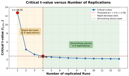
Figure 1.
The critical t-value versus the number of replications. This figure illustrates the rapid decrease in critical values for the first four replications (orange zone) followed by diminishing returns for additional replications (green zone), consistent with the t-distribution properties described in Remark 1. The horizontal dashed line marks the threshold , establishing as the minimum for practical significance testing.
Building on this foundation for hypothesis testing capability, we now examine how partial replication enhances statistical power. The power enhancement achieved through partial replication follows a predictable pattern:
Remark 2
(Power Enhancement Through Replication). The statistical power to detect an effect depends on the degrees of freedom available for error estimation. Using the standard power formula for the t-test, the power to detect a main effect of size δ is given by the following:
where , and denotes the cumulative distribution function of the standard normal distribution.
Numerical evaluation using the non-central t-distribution for DSDs with m factors and standardized effect size yields characteristic power levels. Our comprehensive simulation study (Section 4) confirms these patterns across all factor levels examined:
- 1.
- Basic DSD without replication (): Power is inadequate for practical screening
- Even factors: Power (main effects) .
- Odd factors: Power (main effects) .
- 2.
- Half-partial replication ( runs added): Power reaches acceptable levels
- 3.
- Full replication (): Power approaches the maximum
These patterns demonstrate that substantial power enhancement can be achieved through strategic partial replication without the expense of full replication. A detailed empirical validation across multiple factor levels is presented in Section 4.
Among the various replication strategies examined, the half-partial replication approach emerges as particularly efficient. We formally define this strategy as follows:
Definition 1
(Half-Partial Replication). For a DSD with m factors, the half-partial replication strategy is defined as the augmentation of the basic design with replicated runs, resulting in a total of runs.
Experimental Efficiency Analysis. The half-partial replication strategy (Definition 1) requires the following:
compared to full replication requiring runs. The relative experimental efficiency is as follows:
For large m, where , we can evaluate the asymptotic efficiency:
Dividing both the numerator and denominator by m, we obtain the following:
Thus, half-partial replication asymptotically requires only of the experimental runs compared to full replication, representing substantial experimental economy.
Remark 3
(Empirical Power–Efficiency Performance). Our comprehensive simulation study (Section 4) demonstrates that the half-partial replication strategy achieves exceptional power–efficiency performance:
- 1.
- For the detection of main effects, (half-partial achieves at least 90% of full replication power).
- 2.
- The efficiency-power ratio: (power retention exceeds run reduction by more than 40%).
These empirical findings demonstrate that half-partial replication achieves at least 90% of the power of full replication while requiring only approximately 62.5% of the experimental runs. This represents superlinear returns relative to experimental investment: you retain more statistical power than the proportion of runs you keep. The combination of demonstrated experimental efficiency (requiring 62.5% of runs) and empirically validated high statistical power makes half-partial replication a highly effective practical strategy for resource-constrained screening experiments.
Remark 4
(Practical Replication Guidelines). Based on statistical principles and our empirical investigation, we provide the following guidance for selecting replication strategies:
- Minimum replication: Always include at least four replicated runs to ensure (Remark 1), making effect detection practically feasible. With fewer than four replicates, the critical value exceeds 3.18, requiring effects to be more than three times their standard error for significance.
- Recommended strategy: Implement half-partial replication (Definition 1) for efficient experimental design, achieving near full replication power (Remark 2) with substantially fewer runs. This strategy provides an excellent balance between statistical power and resource constraints.
- Case selection: Case 1 (balanced replication) exhibits lower relative standard errors for quadratic effect estimates, making it preferable when the accurate estimation of curvature is paramount. Case 2 (unbalanced replication) reduces correlation among effect estimates as replication increases, beneficial when orthogonality is prioritized.
- Efficiency trade-off: The modest efficiency losses from replication (D-efficiency and A-efficiency decrease slightly) are offset by substantial gains in estimation precision and hypothesis testing capability, as demonstrated in Section 4.
These statistical foundations and efficiency considerations provide the framework for our comprehensive empirical investigation, which systematically evaluates partial replication performance across multiple factor levels (Section 4).
3.2. Empirical Investigation
To validate these theoretical predictions and explore practical implementation, we investigate eight and seven factors, representing even and odd factors, respectively. While we present detailed results for 7 and 8 factors as representative cases in the main text, our investigation encompasses the full range of even factors (6, 8, 10, 12) and odd factors (5, 7, 9, 11). The DSD with 12 factors comprises 25 runs, representing a substantial screening experiment in industrial practice. The patterns observed for seven and eight factors—particularly the critical role of achieving at least four replicated runs, the power enhancement characteristics, and the efficiency of half-partial replication—hold consistently across all factor levels examined. The comprehensive power, RSE, D-efficiency, and A-efficiency results for all factor combinations are provided in the appendices, ensuring the complete documentation of our findings. This range of 5 to 12 factors (corresponding to 11 to 25 base runs) covers the majority of practical screening applications, where experimenters seek to identify active factors among a moderately large set while maintaining experimental feasibility.
Throughout this study, we consider the selection of two, four, six, and eight additional replicated runs under two replication strategies: Case 1 (balanced replication), where replicated runs preserve the orthogonal structure of the design matrix, and Case 2 (unbalanced replication), which prioritizes minimizing correlation among effect estimates. The design structures for eight and seven factors with two, four, six, and eight replicated additional runs are illustrated in Table A1, Table A2, Table A3 and Table A4, respectively.
4. Partially Replicated Result
One can observe, as shown in Figure 2, that both replicated and non-replicated runs for seven factors yield the highest power for the main effects. This outcome is expected, considering the presence of more degrees of freedom. Conversely, for eight factors, both replicated and non-replicated runs begin with power levels below 60 and eventually reach the same power level as that for seven factors. The most significant increase occurs after the replication of four runs. Regarding the quadratic effects, seven factors with replicated runs exhibit the highest power, whereas the power of eight factors with replicated runs sees a substantial increase after replicating four runs.
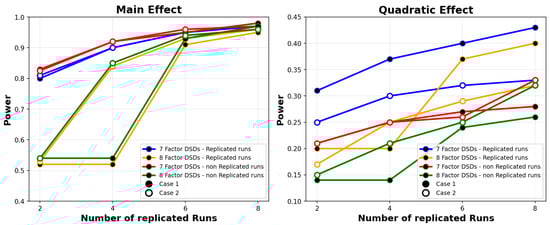
Figure 2.
Power comparison between 7 and 8 factors.
A more comprehensive analysis of Figure 3 uncovers intriguing trends in the relative standard errors (RSEs) concerning main and quadratic effects when comparing designs with seven and eight factors and incorporating replicated runs. For main effects, the RSE exhibits a slight reduction as the number of runs increases, and this trend holds consistently for both seven and eight factors, with no significant disparity between the two cases. In the context of quadratic effects, both designs with seven and eight factors, featuring replicated runs in Case 1 (representing balanced designs), manifest the lowest RSE. This outcome aligns with expectations, as balanced designs generally yield more favorable characteristics, resulting in a decreased RSE.
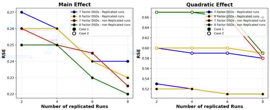
Figure 3.
RSE comparison between 7 and 8 factors.
Examining the max absolute correlation for main effects, shown in Figure 4, the appeal of Case 2 is apparent, as the max absolute correlation decreases, to almost zero, when the number of replicated runs increases. Unfortunately, D-efficiency and A-efficiency, see Figure 5, provide a lower efficiency percentage due to the loss of orthogonality due to the replicated runs.
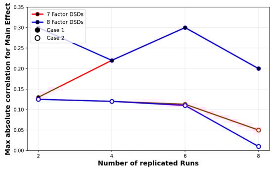
Figure 4.
Comparison of max absolute correlation for main effect between 7 and 8 factors.
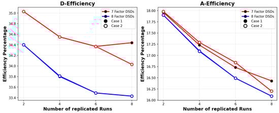
Figure 5.
Comparison of D-efficiency and A-efficiency between 7 and 8 factors.
Based on the findings above, our primary focus shifts towards understanding how power, relative standard errors (RSEs), D-efficiency (), and A-efficiency () are influenced by the number of factors, denoted as m within the set . Additionally, the level of replication is designated by three distinct scenarios: “the basic ()”, representing no replication; “half-partial replication,” which involves replicating half of the total runs for each factor without a center point in both cases (); and “the full replication of runs” (), signifying the complete replication of the entire design.
Figure 6 demonstrates that the replication of half the total runs, applicable in both Case 1 and Case 2, significantly enhances the ability to detect main effects, rivaling the performance of full replication. Interestingly, the figure also underscores that Case 1 exhibits superior capability in detecting quadratic effects.
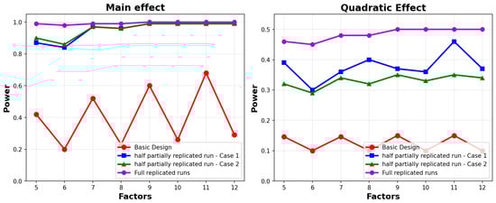
Figure 6.
Power versus the number of factors.
Turning our attention to Figure 7, we observe a consistent trend: the relative standard errors (RSEs) for main effects decrease as the number of factors increases. For quadratic effects, the scenario varies. When we replicate half the runs in Case 1, the RSE is notably lower when there are five factors. In contrast, replicating half the runs in Case 2 yields a lower RSE when there are eight factors. As illustrated in Figure 8, both and decrease as the number of factors increases, irrespective of the replication scenario. This decline can be attributed to the loss of orthogonality, a crucial factor in experimental design efficiency. These observations suggest that the choice of replication and factor configuration should be made thoughtfully to optimize the trade-off between design efficiency and the accuracy of parameter estimates.

Figure 7.
RSE versus the number of factors.
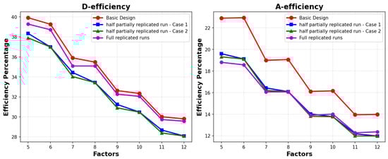
Figure 8.
Designs’ D-efficiency and A-efficiency versus the number of factors.
Design Efficiency and Precision Trade-Offs
Our empirical investigation across designs with factors reveals systematic patterns in the relationship between design efficiency and estimation precision. As illustrated in Figure 8, both D-efficiency and A-efficiency decrease approximately linearly as the number of factors increases, with observed rates of approximately and . This decline can be attributed to the loss of orthogonality when replicated runs are added to the design—a fundamental trade-off in experimental design.
Interestingly, while design efficiency decreases with additional factors, Figure 7 demonstrates that the RSE for main effects improves, decreasing at approximately . This creates an efficiency–precision trade-off ratio of , indicating that efficiency losses outpace precision gains on a percentage basis. However, for industrial applications where detecting the effects of magnitude with power is the primary goal, the precision gains remain sufficient to justify the modest efficiency losses.
Based on the statistical foundations and empirical findings established in this investigation, we recommend the following practical design configuration for experimenters: use a total of runs, with a minimum of replicated runs. The choice between Case 1 (balanced replication) and Case 2 (unbalanced replication) should be guided by specific experimental objectives and the relative importance of different model terms.
Case 1 (Balanced Replication) is recommended when the following conditions are present: (i) Quadratic effects are of primary interest. As demonstrated in Figure 3 and Figure 7, Case 1 consistently yields a lower RSE for quadratic effects across all factor levels examined. For designs with seven and eight factors, balanced replication manifests RSE values approximately 13–15% lower for quadratic terms compared to Case 2 (RSE – versus – with four replications). (ii) Curvature detection is critical to experimental success. When the primary goal emphasizes identifying and accurately quantifying nonlinear relationships between factors and response, the improved precision for quadratic effect estimation becomes essential. (iii) Balanced statistical properties across effect types are valued. Case 1 provides consistent statistical efficiency for both main and quadratic effects, making it suitable when no prior knowledge indicates which effect types are more likely to be active.
Case 2 (Unbalanced Replication) is recommended when the following conditions are present: (i) Orthogonality preservation is paramount. As illustrated in Figure 4, Case 2 demonstrates superior performance in maintaining low correlation between main effects, with the maximum absolute correlations approaching zero as replication increases (being reduced by up to 80% compared to Case 1 at maximum replication). This near-orthogonal structure proves particularly valuable when the independent estimation of main effects is required, multicollinearity concerns must be minimized, or effect estimates need robustness to model misspecification. (ii) Main effects dominate experimental objectives. When screening experiments prioritize the identification of active factors over curvature characterization, Case 2’s superior orthogonality properties become advantageous while maintaining comparable power for main effects (Table A5 and Table A6 demonstrate a power for both cases with half-partial replication). (iii) Follow-up experimentation is planned. When the current experiment serves as initial screening with anticipated follow-up studies for detailed modeling, Case 2’s excellent orthogonality facilitates reliable factor identification in the screening phase.
Practical trade-offs and default recommendation: Both strategies achieve comparable statistical power for main effects, reaching 0.90–0.95 with half-partial replication, as shown in Figure 6. The primary differentiation lies in the RSE for quadratic effects (Case 1’s advantage of 13–15%) versus orthogonality (Case 2’s advantage with correlation reductions up to 80%). D-efficiency and A-efficiency show minimal practical differences between cases (Figure 5), with both maintaining acceptable efficiency levels. For experimenters uncertain about which strategy to employ, we recommend Case 1 as the default choice due to its balanced properties and superior quadratic effect precision. However, when orthogonality is explicitly valued or main effects clearly constitute the priority, Case 2 offers compelling advantages. The relatively minor differences in overall design optimality allow practitioners flexibility to prioritize based on their specific experimental context.
5. Conclusions and Discussion
The results of our study revealed some promising insights. Notably, we observed that as the number of replicated runs increased, there was a noticeable enhancement in statistical power. This heightened power equips experimenters with a stronger ability to detect main effects and quadratic effects, a critical factor in robust experimental design.
Additionally, we found that relative standard errors (RSEs) displayed a consistent downward trend with increased replication. This reduction in the RSE is a significant advantage as it implies that parameter estimates become more accurate and reliable as the replication level rises. A decrease in the RSE can lead to greater confidence in the results and ultimately more sound conclusions drawn from the experiments.
Based on these empirical and theoretical considerations, we propose a strategic recommendation for experimenters. The judicious utilization of the half-partial replication strategy emerged as a winning approach. This methodology not only augments experimental performance but also eliminates the logistical complexities and resource-intensive requirements often associated with the full replication of the entire design.
Our statistical foundations and empirical findings provide strong evidence-based justification for these recommendations. Remark 1 establishes the statistical principles underlying the critical importance of achieving at least four replicated runs for practical hypothesis testing, while the efficiency analysis demonstrates that half-partial replication achieves excellent experimental economy, requiring only 62.5% of the runs needed for full replication while retaining at least 90% of its statistical power for the detection of main effects.
In summary, our findings provide valuable guidance to researchers and experimenters seeking to optimize the design of Definitive Screening Experiments. By harnessing the power of partial replication, they can navigate the complex landscape of experimental design with precision and confidence.
Our recommendations offer a practical road-map to the efficient and effective use of definitive screening designs, ensuring robust and insightful outcomes. It is our hope that this study serves as a valuable resource for those dedicated to extracting the greatest insights from their experimental endeavors.
Building on the findings of this research, several promising avenues for future investigations come to light. First, exploring the application of advanced statistical techniques to assess the efficiency and power in more complex experimental designs could yield valuable insights. Additionally, the impact of varying degrees of partial replication, such as one-third or two-thirds replication, on experimental outcomes remains largely uncharted territory. Investigating the integration of partial replication strategies with modern computational tools and machine learning algorithms for automated experiment design could further streamline the process. Moreover, considering the interplay between partial replication and other factors like sample size, cost constraints, and the nature of the factors under investigation opens doors for multifaceted analyses. These future research directions hold the potential to advance the field of experimental design and empower experimenters with even more effective tools for optimizing their studies.
Furthermore, this study lays the groundwork for the exploration of hybrid experimental designs that combine partial replication with other advanced design methodologies. Investigating the synergy between partial replication and techniques like factorial designs, response surface methodologies, or mixture experiments could uncover innovative strategies for optimizing the efficiency and power of experiments across various domains. Additionally, the study of adaptive experimental designs that dynamically adjust replication based on ongoing results could enhance the efficiency and cost-effectiveness of research. Investigating the integration of partial replication within the framework of multi-stage experimental setups and longitudinal studies may provide novel insights into the optimal design of complex experiments. These evolving research avenues offer the potential to revolutionize experimental design practices and propel them into new frontiers of efficiency and effectiveness. The scope of this investigation—covering even factors from 6 to 12 and odd factors from 5 to 11—represents a comprehensive range for screening experiments in industrial and scientific applications. A DSD with 12 factors requires 25 runs in its basic form, which already represents a substantial experimental commitment. Our findings demonstrate that partial replication strategies, particularly half-partial replication, provide a systematic approach to enhancing statistical power and precision across this entire range. The patterns observed for seven and eight factors—particularly the critical role of achieving at least four replicated runs, the power enhancement characteristics, and the efficiency of half-partial replication—hold consistently across all factor levels examined. The comprehensive power, RSE, D-efficiency, and A-efficiency results for all factor combinations provide the complete documentation of these findings. The principles established here extend naturally to larger designs and offer practitioners evidence-based guidance for balancing statistical rigor with experimental economy in screening experiments.
Author Contributions
Conceptualization, M.H.A. and B.S.O.A.; methodology, B.S.O.A.; software, B.S.O.A.; validation, M.H.A. and B.S.O.A.; formal analysis, M.H.A.; investigation, M.H.A. and B.S.O.A.; resources, M.H.A.; data curation, B.S.O.A.; writing—original draft preparation, M.H.A.; writing—review and editing, M.H.A. and B.S.O.A.; visualization, B.S.O.A.; supervision, M.H.A.; project administration, B.S.O.A. All authors have read and agreed to the published version of the manuscript.
Funding
This research received no external funding.
Data Availability Statement
The raw data supporting the conclusions of this article will be made available by the authors on request.
Conflicts of Interest
The authors declare no conflicts of interest.
Appendix A. The Construction of the Proposed Design
Table A1.
Eight- and seven-factor augmented with 2 additional runs in Cases 1 and 2.
Table A1.
Eight- and seven-factor augmented with 2 additional runs in Cases 1 and 2.
| Factor | 8 | 7 | Factor | 8 | 7 | ||||||||||||||||||||||||||
|---|---|---|---|---|---|---|---|---|---|---|---|---|---|---|---|---|---|---|---|---|---|---|---|---|---|---|---|---|---|---|---|
| Case | 1 | 1 | Case | 2 | 2 | ||||||||||||||||||||||||||
| Run | Run | ||||||||||||||||||||||||||||||
| ⁎ 1 | 0 | 1 | 1 | 1 | 1 | 1 | 1 | 1 | 0 | 1 | 1 | 1 | 1 | 1 | 1 | ⁎ 1 | 0 | 1 | 1 | 1 | 1 | 1 | 1 | 1 | 0 | 1 | 1 | 1 | 1 | 1 | 1 |
| ⁎ 2 | 0 | 1 | 1 | 1 | 1 | 1 | 1 | 1 | 0 | 1 | 1 | 1 | 1 | 1 | 1 | ⁎ 2 | 0 | 1 | 1 | 1 | 1 | 1 | 1 | 1 | 0 | 1 | 1 | 1 | 1 | 1 | 1 |
| ⁎ 3 | 0 | −1 | −1 | −1 | −1 | −1 | −1 | −1 | 0 | −1 | −1 | −1 | −1 | −1 | −1 | 3 | 0 | −1 | −1 | −1 | −1 | −1 | −1 | −1 | 0 | −1 | −1 | −1 | −1 | −1 | −1 |
| ⁎ 4 | 0 | −1 | −1 | −1 | −1 | −1 | −1 | −1 | 0 | −1 | −1 | −1 | −1 | −1 | −1 | ⁎ 4 | 1 | 0 | 1 | 1 | −1 | 1 | −1 | −1 | 1 | 0 | 1 | 1 | −1 | 1 | −1 |
| 5 | 1 | 0 | 1 | 1 | −1 | 1 | −1 | −1 | 1 | 0 | 1 | 1 | −1 | 1 | −1 | ⁎ 5 | 1 | 0 | 1 | 1 | −1 | 1 | −1 | −1 | 1 | 0 | 1 | 1 | −1 | 1 | −1 |
| 6 | −1 | 0 | −1 | −1 | 1 | −1 | 1 | 1 | −1 | 0 | −1 | −1 | 1 | −1 | 1 | 6 | −1 | 0 | −1 | −1 | 1 | −1 | 1 | 1 | −1 | 0 | −1 | −1 | 1 | −1 | 1 |
| 7 | 1 | −1 | 0 | 1 | 1 | −1 | 1 | −1 | 1 | −1 | 0 | 1 | 1 | −1 | 1 | 7 | 1 | −1 | 0 | 1 | 1 | −1 | 1 | −1 | 1 | −1 | 0 | 1 | 1 | −1 | 1 |
| 8 | −1 | 1 | 0 | −1 | −1 | 1 | −1 | 1 | −1 | 1 | 0 | −1 | −1 | 1 | −1 | 8 | −1 | 1 | 0 | −1 | −1 | 1 | −1 | 1 | −1 | 1 | 0 | −1 | −1 | 1 | −1 |
| 9 | 1 | −1 | −1 | 0 | 1 | 1 | −1 | 1 | 1 | −1 | −1 | 0 | 1 | 1 | −1 | 9 | 1 | −1 | −1 | 0 | 1 | 1 | −1 | 1 | 1 | −1 | −1 | 0 | 1 | 1 | −1 |
| 10 | −1 | 1 | 1 | 0 | −1 | −1 | 1 | −1 | −1 | 1 | 1 | 0 | −1 | −1 | 1 | 10 | −1 | 1 | 1 | 0 | −1 | −1 | 1 | −1 | −1 | 1 | 1 | 0 | −1 | −1 | 1 |
| 11 | 1 | 1 | −1 | −1 | 0 | 1 | 1 | −1 | 1 | 1 | −1 | −1 | 0 | 1 | 1 | 11 | 1 | 1 | −1 | −1 | 0 | 1 | 1 | −1 | 1 | 1 | −1 | −1 | 0 | 1 | 1 |
| 12 | −1 | −1 | 1 | 1 | 0 | −1 | −1 | 1 | −1 | −1 | 1 | 1 | 0 | −1 | −1 | 12 | −1 | −1 | 1 | 1 | 0 | −1 | −1 | 1 | −1 | −1 | 1 | 1 | 0 | −1 | −1 |
| 13 | 1 | −1 | 1 | −1 | −1 | 0 | 1 | 1 | 1 | −1 | 1 | −1 | −1 | 0 | 1 | 13 | 1 | −1 | 1 | −1 | −1 | 0 | 1 | 1 | 1 | −1 | 1 | −1 | −1 | 0 | 1 |
| 14 | −1 | 1 | −1 | 1 | 1 | 0 | −1 | −1 | −1 | 1 | −1 | 1 | 1 | 0 | −1 | 14 | −1 | 1 | −1 | 1 | 1 | 0 | −1 | −1 | −1 | 1 | −1 | 1 | 1 | 0 | −1 |
| 15 | 1 | 1 | −1 | 1 | −1 | −1 | 0 | 1 | 1 | 1 | −1 | 1 | −1 | −1 | 0 | 15 | 1 | 1 | −1 | 1 | −1 | −1 | 0 | 1 | 1 | 1 | −1 | 1 | −1 | −1 | 0 |
| 16 | −1 | −1 | 1 | −1 | 1 | 1 | 0 | −1 | −1 | −1 | 1 | −1 | 1 | 1 | 0 | 16 | −1 | −1 | 1 | −1 | 1 | 1 | 0 | −1 | −1 | −1 | 1 | −1 | 1 | 1 | 0 |
| 17 | 1 | 1 | 1 | −1 | 1 | −1 | −1 | 0 | 1 | 1 | 1 | −1 | 1 | −1 | −1 | 17 | 1 | 1 | 1 | −1 | 1 | −1 | −1 | 0 | 1 | 1 | 1 | −1 | 1 | −1 | −1 |
| 18 | −1 | −1 | −1 | 1 | −1 | 1 | 1 | 0 | −1 | −1 | −1 | 1 | −1 | 1 | 1 | 18 | −1 | −1 | −1 | 1 | −1 | 1 | 1 | 0 | −1 | −1 | −1 | 1 | −1 | 1 | 1 |
| 19 | 0 | 0 | 0 | 0 | 0 | 0 | 0 | 0 | 0 | 0 | 0 | 0 | 0 | 0 | 0 | 19 | 0 | 0 | 0 | 0 | 0 | 0 | 0 | 0 | 0 | 0 | 0 | 0 | 0 | 0 | 0 |
| * Indicates replicated rows. | |||||||||||||||||||||||||||||||
Table A2.
Eight- and seven-factor augmented with 4 additional runs in Cases 1 and 2.
Table A2.
Eight- and seven-factor augmented with 4 additional runs in Cases 1 and 2.
| Factor | 8 | 7 | Factor | 8 | 7 | ||||||||||||||||||||||||||
|---|---|---|---|---|---|---|---|---|---|---|---|---|---|---|---|---|---|---|---|---|---|---|---|---|---|---|---|---|---|---|---|
| Case | 1 | 1 | Case | 2 | 2 | ||||||||||||||||||||||||||
| Run | Run | ||||||||||||||||||||||||||||||
| ⁎ 1 | 0 | 1 | 1 | 1 | 1 | 1 | 1 | 1 | 0 | 1 | 1 | 1 | 1 | 1 | 1 | ⁎ 1 | 0 | 1 | 1 | 1 | 1 | 1 | 1 | 1 | 0 | 1 | 1 | 1 | 1 | 1 | 1 |
| ⁎ 2 | 0 | 1 | 1 | 1 | 1 | 1 | 1 | 1 | 0 | 1 | 1 | 1 | 1 | 1 | 1 | ⁎ 2 | 0 | 1 | 1 | 1 | 1 | 1 | 1 | 1 | 0 | 1 | 1 | 1 | 1 | 1 | 1 |
| ⁎ 3 | 0 | −1 | −1 | −1 | −1 | −1 | −1 | −1 | 0 | −1 | −1 | −1 | −1 | −1 | −1 | 3 | 0 | −1 | −1 | −1 | −1 | −1 | −1 | −1 | 0 | −1 | −1 | −1 | −1 | −1 | −1 |
| ⁎ 4 | 0 | −1 | −1 | −1 | −1 | −1 | −1 | −1 | 0 | −1 | −1 | −1 | −1 | −1 | −1 | ⁎ 4 | 1 | 0 | 1 | 1 | −1 | 1 | −1 | −1 | 1 | 0 | 1 | 1 | −1 | 1 | −1 |
| ⁎ 5 | 1 | 0 | 1 | 1 | −1 | 1 | −1 | −1 | 1 | 0 | 1 | 1 | −1 | 1 | −1 | ⁎ 5 | 1 | 0 | 1 | 1 | −1 | 1 | −1 | −1 | 1 | 0 | 1 | 1 | −1 | 1 | −1 |
| ⁎ 6 | 1 | 0 | 1 | 1 | −1 | 1 | −1 | −1 | 1 | 0 | 1 | 1 | −1 | 1 | −1 | 6 | −1 | 0 | −1 | −1 | 1 | −1 | 1 | 1 | −1 | 0 | −1 | −1 | 1 | −1 | 1 |
| ⁎ 7 | −1 | 0 | −1 | −1 | 1 | −1 | 1 | 1 | −1 | 0 | −1 | −1 | 1 | −1 | 1 | ⁎ 7 | 1 | −1 | 0 | 1 | 1 | −1 | 1 | −1 | 1 | −1 | 0 | 1 | 1 | −1 | 1 |
| ⁎ 8 | −1 | 0 | −1 | −1 | 1 | −1 | 1 | 1 | −1 | 0 | −1 | −1 | 1 | −1 | 1 | ⁎ 8 | 1 | −1 | 0 | 1 | 1 | −1 | 1 | −1 | 1 | −1 | 0 | 1 | 1 | −1 | 1 |
| 9 | 1 | −1 | 0 | 1 | 1 | −1 | 1 | −1 | 1 | −1 | 0 | 1 | 1 | −1 | 1 | 9 | −1 | 1 | 0 | −1 | −1 | 1 | −1 | 1 | −1 | 1 | 0 | −1 | −1 | 1 | −1 |
| 10 | −1 | 1 | 0 | −1 | −1 | 1 | −1 | 1 | −1 | 1 | 0 | −1 | −1 | 1 | −1 | ⁎ 10 | 1 | −1 | −1 | 0 | 1 | 1 | −1 | 1 | 1 | −1 | −1 | 0 | 1 | 1 | −1 |
| 11 | 1 | −1 | −1 | 0 | 1 | 1 | −1 | 1 | 1 | −1 | −1 | 0 | 1 | 1 | −1 | ⁎ 11 | 1 | −1 | −1 | 0 | 1 | 1 | −1 | 1 | 1 | −1 | −1 | 0 | 1 | 1 | −1 |
| 12 | −1 | 1 | 1 | 0 | −1 | −1 | 1 | −1 | −1 | 1 | 1 | 0 | −1 | −1 | 1 | 12 | −1 | 1 | 1 | 0 | −1 | −1 | 1 | −1 | −1 | 1 | 1 | 0 | −1 | −1 | 1 |
| 13 | 1 | 1 | −1 | −1 | 0 | 1 | 1 | −1 | 1 | 1 | −1 | −1 | 0 | 1 | 1 | 13 | 1 | 1 | −1 | −1 | 0 | 1 | 1 | −1 | 1 | 1 | −1 | −1 | 0 | 1 | 1 |
| 14 | −1 | −1 | 1 | 1 | 0 | −1 | −1 | 1 | −1 | −1 | 1 | 1 | 0 | −1 | −1 | 14 | −1 | −1 | 1 | 1 | 0 | −1 | −1 | 1 | −1 | −1 | 1 | 1 | 0 | −1 | −1 |
| 15 | 1 | −1 | 1 | −1 | −1 | 0 | 1 | 1 | 1 | −1 | 1 | −1 | −1 | 0 | 1 | 15 | 1 | −1 | 1 | −1 | −1 | 0 | 1 | 1 | 1 | −1 | 1 | −1 | −1 | 0 | 1 |
| 16 | −1 | 1 | −1 | 1 | 1 | 0 | −1 | −1 | −1 | 1 | −1 | 1 | 1 | 0 | −1 | 16 | −1 | 1 | −1 | 1 | 1 | 0 | −1 | −1 | −1 | 1 | −1 | 1 | 1 | 0 | −1 |
| 17 | 1 | 1 | −1 | 1 | −1 | −1 | 0 | 1 | 1 | 1 | −1 | 1 | −1 | −1 | 0 | 17 | 1 | 1 | −1 | 1 | −1 | −1 | 0 | 1 | 1 | 1 | −1 | 1 | −1 | −1 | 0 |
| 18 | −1 | −1 | 1 | −1 | 1 | 1 | 0 | −1 | −1 | −1 | 1 | −1 | 1 | 1 | 0 | 18 | −1 | −1 | 1 | −1 | 1 | 1 | 0 | −1 | −1 | −1 | 1 | −1 | 1 | 1 | 0 |
| 19 | 1 | 1 | 1 | −1 | 1 | −1 | −1 | 0 | 1 | 1 | 1 | −1 | 1 | −1 | −1 | 19 | 1 | 1 | 1 | −1 | 1 | −1 | −1 | 0 | 1 | 1 | 1 | −1 | 1 | −1 | −1 |
| 20 | −1 | −1 | −1 | 1 | −1 | 1 | 1 | 0 | −1 | −1 | −1 | 1 | −1 | 1 | 1 | 20 | −1 | −1 | −1 | 1 | −1 | 1 | 1 | 0 | −1 | −1 | −1 | 1 | −1 | 1 | 1 |
| 21 | 0 | 0 | 0 | 0 | 0 | 0 | 0 | 0 | 0 | 0 | 0 | 0 | 0 | 0 | 0 | 21 | 0 | 0 | 0 | 0 | 0 | 0 | 0 | 0 | 0 | 0 | 0 | 0 | 0 | 0 | 0 |
| * Indicates replicated rows. | |||||||||||||||||||||||||||||||
Table A3.
Eight- and seven-factor augmented with 6 additional runs in Cases 1 and 2.
Table A3.
Eight- and seven-factor augmented with 6 additional runs in Cases 1 and 2.
| Factor | 8 | 7 | Factor | 8 | 7 | ||||||||||||||||||||||||||
|---|---|---|---|---|---|---|---|---|---|---|---|---|---|---|---|---|---|---|---|---|---|---|---|---|---|---|---|---|---|---|---|
| Case | 1 | 1 | Case | 2 | 2 | ||||||||||||||||||||||||||
| Run | Run | ||||||||||||||||||||||||||||||
| ⁎ 1 | 0 | 1 | 1 | 1 | 1 | 1 | 1 | 1 | 0 | 1 | 1 | 1 | 1 | 1 | 1 | ⁎ 1 | 0 | 1 | 1 | 1 | 1 | 1 | 1 | 1 | 0 | 1 | 1 | 1 | 1 | 1 | 1 |
| ⁎ 2 | 0 | 1 | 1 | 1 | 1 | 1 | 1 | 1 | 0 | 1 | 1 | 1 | 1 | 1 | 1 | ⁎ 2 | 0 | 1 | 1 | 1 | 1 | 1 | 1 | 1 | 0 | 1 | 1 | 1 | 1 | 1 | 1 |
| ⁎ 3 | 0 | −1 | −1 | −1 | −1 | −1 | −1 | −1 | 0 | −1 | −1 | −1 | −1 | −1 | −1 | 3 | 0 | −1 | −1 | −1 | −1 | −1 | −1 | −1 | 0 | −1 | −1 | −1 | −1 | −1 | −1 |
| ⁎ 4 | 0 | −1 | −1 | −1 | −1 | −1 | −1 | −1 | 0 | −1 | −1 | −1 | −1 | −1 | −1 | ⁎ 4 | 1 | 0 | 1 | 1 | −1 | 1 | −1 | −1 | 1 | 0 | 1 | 1 | −1 | 1 | −1 |
| ⁎ 5 | 1 | 0 | 1 | 1 | −1 | 1 | −1 | −1 | 1 | 0 | 1 | 1 | −1 | 1 | −1 | ⁎ 5 | 1 | 0 | 1 | 1 | −1 | 1 | −1 | −1 | 1 | 0 | 1 | 1 | −1 | 1 | −1 |
| ⁎ 6 | 1 | 0 | 1 | 1 | −1 | 1 | −1 | −1 | 1 | 0 | 1 | 1 | −1 | 1 | −1 | 6 | −1 | 0 | −1 | −1 | 1 | −1 | 1 | 1 | −1 | 0 | −1 | −1 | 1 | −1 | 1 |
| ⁎ 7 | −1 | 0 | −1 | −1 | 1 | −1 | 1 | 1 | −1 | 0 | −1 | −1 | 1 | −1 | 1 | ⁎ 7 | 1 | −1 | 0 | 1 | 1 | −1 | 1 | −1 | 1 | −1 | 0 | 1 | 1 | −1 | 1 |
| ⁎ 8 | −1 | 0 | −1 | −1 | 1 | −1 | 1 | 1 | −1 | 0 | −1 | −1 | 1 | −1 | 1 | ⁎ 8 | 1 | −1 | 0 | 1 | 1 | −1 | 1 | −1 | 1 | −1 | 0 | 1 | 1 | −1 | 1 |
| ⁎ 9 | 1 | −1 | 0 | 1 | 1 | −1 | 1 | −1 | 1 | −1 | 0 | 1 | 1 | −1 | 1 | 9 | −1 | 1 | 0 | −1 | −1 | 1 | −1 | 1 | −1 | 1 | 0 | −1 | −1 | 1 | −1 |
| ⁎ 10 | 1 | −1 | 0 | 1 | 1 | −1 | 1 | −1 | 1 | −1 | 0 | 1 | 1 | −1 | 1 | ⁎ 10 | 1 | −1 | −1 | 0 | 1 | 1 | −1 | 1 | 1 | −1 | −1 | 0 | 1 | 1 | −1 |
| ⁎ 11 | −1 | 1 | 0 | −1 | −1 | 1 | −1 | 1 | −1 | 1 | 0 | −1 | −1 | 1 | −1 | ⁎ 11 | 1 | −1 | −1 | 0 | 1 | 1 | −1 | 1 | 1 | −1 | −1 | 0 | 1 | 1 | −1 |
| ⁎ 12 | −1 | 1 | 0 | −1 | −1 | 1 | −1 | 1 | −1 | 1 | 0 | −1 | −1 | 1 | −1 | 12 | −1 | 1 | 1 | 0 | −1 | −1 | 1 | −1 | −1 | 1 | 1 | 0 | −1 | −1 | 1 |
| 13 | 1 | −1 | −1 | 0 | 1 | 1 | −1 | 1 | 1 | −1 | −1 | 0 | 1 | 1 | −1 | ⁎ 13 | 1 | 1 | −1 | −1 | 0 | 1 | 1 | −1 | 1 | 1 | −1 | −1 | 0 | 1 | 1 |
| 14 | −1 | 1 | 1 | 0 | −1 | −1 | 1 | −1 | −1 | 1 | 1 | 0 | −1 | −1 | 1 | ⁎ 14 | 1 | 1 | −1 | −1 | 0 | 1 | 1 | −1 | 1 | 1 | −1 | −1 | 0 | 1 | 1 |
| 15 | 1 | 1 | −1 | −1 | 0 | 1 | 1 | −1 | 1 | 1 | −1 | −1 | 0 | 1 | 1 | 15 | −1 | −1 | 1 | 1 | 0 | −1 | −1 | 1 | −1 | −1 | 1 | 1 | 0 | −1 | −1 |
| 16 | −1 | −1 | 1 | 1 | 0 | −1 | −1 | 1 | −1 | −1 | 1 | 1 | 0 | −1 | −1 | ⁎ 16 | 1 | −1 | 1 | −1 | −1 | 0 | 1 | 1 | 1 | −1 | 1 | −1 | −1 | 0 | 1 |
| 17 | 1 | −1 | 1 | −1 | −1 | 0 | 1 | 1 | 1 | −1 | 1 | −1 | −1 | 0 | 1 | ⁎ 17 | 1 | −1 | 1 | −1 | −1 | 0 | 1 | 1 | 1 | −1 | 1 | −1 | −1 | 0 | 1 |
| 18 | −1 | 1 | −1 | 1 | 1 | 0 | −1 | −1 | −1 | 1 | −1 | 1 | 1 | 0 | −1 | 18 | −1 | 1 | −1 | 1 | 1 | 0 | −1 | −1 | −1 | 1 | −1 | 1 | 1 | 0 | −1 |
| 19 | 1 | 1 | −1 | 1 | −1 | −1 | 0 | 1 | 1 | 1 | −1 | 1 | −1 | −1 | 0 | 19 | 1 | 1 | −1 | 1 | −1 | −1 | 0 | 1 | 1 | 1 | −1 | 1 | −1 | −1 | 0 |
| 20 | −1 | −1 | 1 | −1 | 1 | 1 | 0 | −1 | −1 | −1 | 1 | −1 | 1 | 1 | 0 | 20 | −1 | −1 | 1 | −1 | 1 | 1 | 0 | −1 | −1 | −1 | 1 | −1 | 1 | 1 | 0 |
| 21 | 1 | 1 | 1 | −1 | 1 | −1 | −1 | 0 | 1 | 1 | 1 | −1 | 1 | −1 | −1 | 21 | 1 | 1 | 1 | −1 | 1 | −1 | −1 | 0 | 1 | 1 | 1 | −1 | 1 | −1 | −1 |
| 22 | −1 | −1 | −1 | 1 | −1 | 1 | 1 | 0 | −1 | −1 | −1 | 1 | −1 | 1 | 1 | 22 | −1 | −1 | −1 | 1 | −1 | 1 | 1 | 0 | −1 | −1 | −1 | 1 | −1 | 1 | 1 |
| 23 | 0 | 0 | 0 | 0 | 0 | 0 | 0 | 0 | 0 | 0 | 0 | 0 | 0 | 0 | 0 | 23 | 0 | 0 | 0 | 0 | 0 | 0 | 0 | 0 | 0 | 0 | 0 | 0 | 0 | 0 | 0 |
| * Indicates replicated rows. | |||||||||||||||||||||||||||||||
Table A4.
Eight- and seven-factor augmented with 8 additional runs in Cases 1 and 2.
Table A4.
Eight- and seven-factor augmented with 8 additional runs in Cases 1 and 2.
| Factor | 8 | 7 | Factor | 8 | 7 | ||||||||||||||||||||||||||
|---|---|---|---|---|---|---|---|---|---|---|---|---|---|---|---|---|---|---|---|---|---|---|---|---|---|---|---|---|---|---|---|
| Case | 1 | 1 | Case | 2 | 2 | ||||||||||||||||||||||||||
| Run | Run | ||||||||||||||||||||||||||||||
| ⁎ 1 | 0 | 1 | 1 | 1 | 1 | 1 | 1 | 1 | 0 | 1 | 1 | 1 | 1 | 1 | 1 | ⁎ 1 | 0 | 1 | 1 | 1 | 1 | 1 | 1 | 1 | 0 | 1 | 1 | 1 | 1 | 1 | 1 |
| ⁎ 2 | 0 | 1 | 1 | 1 | 1 | 1 | 1 | 1 | 0 | 1 | 1 | 1 | 1 | 1 | 1 | ⁎ 2 | 0 | 1 | 1 | 1 | 1 | 1 | 1 | 1 | 0 | 1 | 1 | 1 | 1 | 1 | 1 |
| ⁎ 3 | 0 | −1 | −1 | −1 | −1 | −1 | −1 | −1 | 0 | −1 | −1 | −1 | −1 | −1 | −1 | 3 | 0 | −1 | −1 | −1 | −1 | −1 | −1 | −1 | 0 | −1 | −1 | −1 | −1 | −1 | −1 |
| ⁎ 4 | 0 | −1 | −1 | −1 | −1 | −1 | −1 | −1 | 0 | −1 | −1 | −1 | −1 | −1 | −1 | ⁎ 4 | 1 | 0 | 1 | 1 | −1 | 1 | −1 | −1 | 1 | 0 | 1 | 1 | −1 | 1 | −1 |
| ⁎ 5 | 1 | 0 | 1 | 1 | −1 | 1 | −1 | −1 | 1 | 0 | 1 | 1 | −1 | 1 | −1 | ⁎ 5 | 1 | 0 | 1 | 1 | −1 | 1 | −1 | −1 | 1 | 0 | 1 | 1 | −1 | 1 | −1 |
| ⁎ 6 | 1 | 0 | 1 | 1 | −1 | 1 | −1 | −1 | 1 | 0 | 1 | 1 | −1 | 1 | −1 | 6 | −1 | 0 | −1 | −1 | 1 | −1 | 1 | 1 | −1 | 0 | −1 | −1 | 1 | −1 | 1 |
| ⁎ 7 | −1 | 0 | −1 | −1 | 1 | −1 | 1 | 1 | −1 | 0 | −1 | −1 | 1 | −1 | 1 | ⁎ 7 | 1 | −1 | 0 | 1 | 1 | −1 | 1 | −1 | 1 | −1 | 0 | 1 | 1 | −1 | 1 |
| ⁎ 8 | −1 | 0 | −1 | −1 | 1 | −1 | 1 | 1 | −1 | 0 | −1 | −1 | 1 | −1 | 1 | ⁎ 8 | 1 | −1 | 0 | 1 | 1 | −1 | 1 | −1 | 1 | −1 | 0 | 1 | 1 | −1 | 1 |
| ⁎ 9 | 1 | −1 | 0 | 1 | 1 | −1 | 1 | −1 | 1 | −1 | 0 | 1 | 1 | −1 | 1 | 9 | −1 | 1 | 0 | −1 | −1 | 1 | −1 | 1 | −1 | 1 | 0 | −1 | −1 | 1 | −1 |
| ⁎ 10 | 1 | −1 | 0 | 1 | 1 | −1 | 1 | −1 | 1 | −1 | 0 | 1 | 1 | −1 | 1 | ⁎ 10 | 1 | −1 | −1 | 0 | 1 | 1 | −1 | 1 | 1 | −1 | −1 | 0 | 1 | 1 | −1 |
| ⁎ 11 | −1 | 1 | 0 | −1 | −1 | 1 | −1 | 1 | −1 | 1 | 0 | −1 | −1 | 1 | −1 | ⁎ 11 | 1 | −1 | −1 | 0 | 1 | 1 | −1 | 1 | 1 | −1 | −1 | 0 | 1 | 1 | −1 |
| ⁎ 12 | −1 | 1 | 0 | −1 | −1 | 1 | −1 | 1 | −1 | 1 | 0 | −1 | −1 | 1 | −1 | 12 | −1 | 1 | 1 | 0 | −1 | −1 | 1 | −1 | −1 | 1 | 1 | 0 | −1 | −1 | 1 |
| ⁎ 13 | 1 | −1 | −1 | 0 | 1 | 1 | −1 | 1 | 1 | −1 | −1 | 0 | 1 | 1 | −1 | ⁎ 13 | 1 | 1 | −1 | −1 | 0 | 1 | 1 | −1 | 1 | 1 | −1 | −1 | 0 | 1 | 1 |
| ⁎ 14 | 1 | −1 | −1 | 0 | 1 | 1 | −1 | 1 | 1 | −1 | −1 | 0 | 1 | 1 | −1 | ⁎ 14 | 1 | 1 | −1 | −1 | 0 | 1 | 1 | −1 | 1 | 1 | −1 | −1 | 0 | 1 | 1 |
| ⁎ 15 | −1 | 1 | 1 | 0 | −1 | −1 | 1 | −1 | −1 | 1 | 1 | 0 | −1 | −1 | 1 | 15 | −1 | −1 | 1 | 1 | 0 | −1 | −1 | 1 | −1 | −1 | 1 | 1 | 0 | −1 | −1 |
| ⁎ 16 | −1 | 1 | 1 | 0 | −1 | −1 | 1 | −1 | −1 | 1 | 1 | 0 | −1 | −1 | 1 | ⁎ 16 | 1 | −1 | 1 | −1 | −1 | 0 | 1 | 1 | 1 | −1 | 1 | −1 | −1 | 0 | 1 |
| 17 | 1 | 1 | −1 | −1 | 0 | 1 | 1 | −1 | 1 | 1 | −1 | −1 | 0 | 1 | 1 | ⁎ 17 | 1 | −1 | 1 | −1 | −1 | 0 | 1 | 1 | 1 | −1 | 1 | −1 | −1 | 0 | 1 |
| 18 | −1 | −1 | 1 | 1 | 0 | −1 | −1 | 1 | −1 | −1 | 1 | 1 | 0 | −1 | −1 | 18 | −1 | 1 | −1 | 1 | 1 | 0 | −1 | −1 | −1 | 1 | −1 | 1 | 1 | 0 | −1 |
| 19 | 1 | −1 | 1 | −1 | −1 | 0 | 1 | 1 | 1 | −1 | 1 | −1 | −1 | 0 | 1 | ⁎ 19 | 1 | 1 | −1 | 1 | −1 | −1 | 0 | 1 | 1 | 1 | −1 | 1 | −1 | −1 | 0 |
| 20 | −1 | 1 | −1 | 1 | 1 | 0 | −1 | −1 | −1 | 1 | −1 | 1 | 1 | 0 | −1 | ⁎ 20 | 1 | 1 | −1 | 1 | −1 | −1 | 0 | 1 | 1 | 1 | −1 | 1 | −1 | −1 | 0 |
| 21 | 1 | 1 | −1 | 1 | −1 | −1 | 0 | 1 | 1 | 1 | −1 | 1 | −1 | −1 | 0 | 21 | −1 | −1 | 1 | −1 | 1 | 1 | 0 | −1 | −1 | −1 | 1 | −1 | 1 | 1 | 0 |
| 22 | −1 | −1 | 1 | −1 | 1 | 1 | 0 | −1 | −1 | −1 | 1 | −1 | 1 | 1 | 0 | ⁎ 22 | 1 | 1 | 1 | −1 | 1 | −1 | −1 | 0 | 1 | 1 | 1 | −1 | 1 | −1 | −1 |
| 23 | 1 | 1 | 1 | −1 | 1 | −1 | −1 | 0 | 1 | 1 | 1 | −1 | 1 | −1 | −1 | ⁎ 23 | 1 | 1 | 1 | −1 | 1 | −1 | −1 | 0 | 1 | 1 | 1 | −1 | 1 | −1 | −1 |
| 24 | −1 | −1 | −1 | 1 | −1 | 1 | 1 | 0 | −1 | −1 | −1 | 1 | −1 | 1 | 1 | 24 | −1 | −1 | −1 | 1 | −1 | 1 | 1 | 0 | −1 | −1 | −1 | 1 | −1 | 1 | 1 |
| 25 | 0 | 0 | 0 | 0 | 0 | 0 | 0 | 0 | 0 | 0 | 0 | 0 | 0 | 0 | 0 | 25 | 0 | 0 | 0 | 0 | 0 | 0 | 0 | 0 | 0 | 0 | 0 | 0 | 0 | 0 | 0 |
| * Indicates replicated rows. | |||||||||||||||||||||||||||||||
Appendix B. Power and RSE Values
Table A5.
Power and RSE for each term with 8 factors in both cases.
Table A5.
Power and RSE for each term with 8 factors in both cases.
| Case | 1 | 2 | ||||||||||||||
|---|---|---|---|---|---|---|---|---|---|---|---|---|---|---|---|---|
| S | 2 | 4 | 6 | 8 | 2 | 4 | 6 | 8 | ||||||||
| Terms | Power | RSE | Power | RSE | Power | RSE | Power | RSE | Power | RSE | Power | RSE | Power | RSE | Power | RSE |
| 0.09 | 1 | 0.12 | 1 | 0.13 | 1 | 0.14 | 1 | 0.09 | 1 | 0.12 | 1 | 0.14 | 1 | 0.14 | 1 | |
| 0.52 | 0.26 | 0.82 | 0.25 | 0.91 | 0.24 | 0.95 | 0.23 | 0.53 | 0.26 | 0.84 | 0.25 | 0.93 | 0.24 | 0.96 | 0.23 | |
| 0.54 | 0.25 | 0.82 | 0.25 | 0.91 | 0.24 | 0.95 | 0.23 | 0.53 | 0.26 | 0.84 | 0.25 | 0.93 | 0.24 | 0.96 | 0.23 | |
| 0.54 | 0.25 | 0.85 | 0.24 | 0.91 | 0.24 | 0.95 | 0.23 | 0.54 | 0.26 | 0.84 | 0.25 | 0.93 | 0.24 | 0.96 | 0.23 | |
| 0.54 | 0.25 | 0.85 | 0.24 | 0.93 | 0.23 | 0.95 | 0.23 | 0.54 | 0.26 | 0.84 | 0.25 | 0.93 | 0.24 | 0.96 | 0.23 | |
| 0.54 | 0.25 | 0.85 | 0.24 | 0.93 | 0.23 | 0.97 | 0.22 | 0.54 | 0.26 | 0.85 | 0.25 | 0.93 | 0.24 | 0.96 | 0.23 | |
| 0.54 | 0.25 | 0.85 | 0.24 | 0.93 | 0.23 | 0.97 | 0.22 | 0.54 | 0.26 | 0.85 | 0.25 | 0.93 | 0.24 | 0.96 | 0.23 | |
| 0.54 | 0.25 | 0.85 | 0.24 | 0.93 | 0.23 | 0.97 | 0.22 | 0.54 | 0.26 | 0.85 | 0.25 | 0.94 | 0.24 | 0.96 | 0.23 | |
| 0.54 | 0.25 | 0.85 | 0.24 | 0.93 | 0.23 | 0.97 | 0.22 | 0.54 | 0.26 | 0.85 | 0.25 | 0.94 | 0.24 | 0.96 | 0.23 | |
| 0.2 | 0.52 | 0.31 | 0.52 | 0.37 | 0.51 | 0.4 | 0.51 | 0.17 | 0.6 | 0.25 | 0.6 | 0.29 | 0.6 | 0.32 | 0.59 | |
| 0.14 | 0.67 | 0.31 | 0.52 | 0.37 | 0.51 | 0.4 | 0.51 | 0.17 | 0.6 | 0.25 | 0.6 | 0.29 | 0.6 | 0.32 | 0.59 | |
| 0.14 | 0.67 | 0.21 | 0.67 | 0.37 | 0.51 | 0.4 | 0.51 | 0.15 | 0.67 | 0.25 | 0.6 | 0.29 | 0.6 | 0.32 | 0.59 | |
| 0.14 | 0.67 | 0.21 | 0.67 | 0.24 | 0.66 | 0.4 | 0.51 | 0.15 | 0.67 | 0.25 | 0.6 | 0.29 | 0.6 | 0.32 | 0.59 | |
| 0.14 | 0.67 | 0.21 | 0.67 | 0.24 | 0.66 | 0.26 | 0.66 | 0.15 | 0.67 | 0.21 | 0.67 | 0.29 | 0.6 | 0.32 | 0.59 | |
| 0.14 | 0.67 | 0.21 | 0.67 | 0.24 | 0.66 | 0.26 | 0.66 | 0.15 | 0.67 | 0.21 | 0.67 | 0.29 | 0.6 | 0.32 | 0.59 | |
| 0.14 | 0.67 | 0.21 | 0.67 | 0.24 | 0.66 | 0.26 | 0.66 | 0.15 | 0.67 | 0.21 | 0.67 | 0.25 | 0.67 | 0.32 | 0.59 | |
| 0.14 | 0.67 | 0.21 | 0.67 | 0.24 | 0.66 | 0.26 | 0.66 | 0.15 | 0.67 | 0.21 | 0.67 | 0.25 | 0.67 | 0.32 | 0.59 | |
Table A6.
Power and RSE for each term with 7 factors in both cases.
Table A6.
Power and RSE for each term with 7 factors in both cases.
| Case | 1 | 2 | ||||||||||||||
|---|---|---|---|---|---|---|---|---|---|---|---|---|---|---|---|---|
| S | 2 | 4 | 6 | 8 | 2 | 4 | 6 | 8 | ||||||||
| Terms | Power | RSE | Power | RSE | Power | RSE | Power | RSE | Power | RSE | Power | RSE | Power | RSE | Power | RSE |
| Intercept | 0.13 | 0.98 | 0.14 | 0.97 | 0.15 | 0.98 | 0.15 | 0.98 | 0.13 | 0.98 | 0.14 | 0.98 | 0.15 | 0.98 | 0.154 | 0.97 |
| 0.8 | 0.27 | 0.9 | 0.26 | 0.95 | 0.24 | 0.97 | 0.24 | 0.81 | 0.26 | 0.9 | 0.25 | 0.95 | 0.24 | 0.972 | 0.231 | |
| 0.83 | 0.26 | 0.9 | 0.26 | 0.95 | 0.24 | 0.97 | 0.24 | 0.81 | 0.26 | 0.9 | 0.25 | 0.95 | 0.24 | 0.974 | 0.23 | |
| 0.83 | 0.26 | 0.92 | 0.25 | 0.94 | 0.25 | 0.97 | 0.24 | 0.82 | 0.26 | 0.9 | 0.25 | 0.95 | 0.24 | 0.974 | 0.23 | |
| 0.83 | 0.26 | 0.92 | 0.25 | 0.96 | 0.24 | 0.97 | 0.24 | 0.82 | 0.26 | 0.9 | 0.25 | 0.95 | 0.24 | 0.975 | 0.229 | |
| 0.83 | 0.26 | 0.92 | 0.25 | 0.96 | 0.24 | 0.98 | 0.22 | 0.83 | 0.26 | 0.92 | 0.25 | 0.95 | 0.24 | 0.974 | 0.23 | |
| 0.83 | 0.26 | 0.92 | 0.25 | 0.96 | 0.24 | 0.98 | 0.22 | 0.82 | 0.26 | 0.92 | 0.25 | 0.95 | 0.24 | 0.975 | 0.229 | |
| 0.83 | 0.26 | 0.92 | 0.25 | 0.96 | 0.24 | 0.98 | 0.23 | 0.83 | 0.26 | 0.92 | 0.25 | 0.96 | 0.24 | 0.975 | 0.229 | |
| 0.31 | 0.53 | 0.37 | 0.52 | 0.4 | 0.51 | 0.43 | 0.51 | 0.25 | 0.6 | 0.3 | 0.59 | 0.32 | 0.59 | 0.339 | 0.586 | |
| 0.21 | 0.67 | 0.37 | 0.52 | 0.4 | 0.51 | 0.43 | 0.51 | 0.25 | 0.6 | 0.3 | 0.59 | 0.32 | 0.59 | 0.342 | 0.583 | |
| 0.21 | 0.67 | 0.25 | 0.67 | 0.4 | 0.51 | 0.43 | 0.51 | 0.21 | 0.67 | 0.3 | 0.59 | 0.32 | 0.59 | 0.342 | 0.583 | |
| 0.21 | 0.67 | 0.25 | 0.67 | 0.27 | 0.66 | 0.43 | 0.51 | 0.21 | 0.67 | 0.3 | 0.59 | 0.32 | 0.59 | 0.339 | 0.586 | |
| 0.21 | 0.67 | 0.25 | 0.67 | 0.27 | 0.66 | 0.28 | 0.66 | 0.21 | 0.67 | 0.25 | 0.67 | 0.32 | 0.59 | 0.342 | 0.583 | |
| 0.21 | 0.67 | 0.25 | 0.67 | 0.27 | 0.66 | 0.28 | 0.66 | 0.21 | 0.67 | 0.25 | 0.67 | 0.32 | 0.59 | 0.339 | 0.586 | |
| 0.21 | 0.67 | 0.25 | 0.67 | 0.27 | 0.66 | 0.28 | 0.66 | 0.21 | 0.67 | 0.25 | 0.67 | 0.27 | 0.66 | 0.339 | 0.586 | |
References
- Dean, A.M.; Lewis, S.M. (Eds.) Screening: Methods for Experimentation in Industry, Drug Discovery, and Genetics; Springer: New York, NY, USA, 2006. [Google Scholar]
- Box, G.E.P.; Hunter, J.S. The 2k−p Fractional Factorial Designs Part I. Technometrics 1961, 3, 311–351. [Google Scholar]
- Plackett, R.L.; Burman, J.P. The Design of Optimum Multifactorial Experiments. Biometrika 1946, 33, 305–325. [Google Scholar] [CrossRef]
- Jones, B.; Nachtsheim, C.J. A class of three-level designs for definitive screening in the presence of second order effects. J. Qual. Technol. 2011, 43, 1–15. [Google Scholar] [CrossRef]
- Xiao, L.; Lin, D.K.J.; Bai, F. Constructing definitive screening designs using conference matrices. J. Qual. Technol. 2012, 44, 2–8. [Google Scholar] [CrossRef]
- Georgiou, S.D.; Stylianou, S.; Aggarwal, M. Efficient three-level screening designs using weighing matrices. Statistics 2014, 48, 815–833. [Google Scholar] [CrossRef]
- Jones, B.; Nachtsheim, C.J. Efficient designs with minimal aliasing. Technometrics 2011, 53, 62–71. [Google Scholar] [CrossRef]
- Jones, B.; Nachtsheim, C.J. Definitive screening designs with added two-level categorical factors. J. Qual. Technol. 2013, 45, 121–129. [Google Scholar] [CrossRef]
- Jones, B.; Montgomery, D.C. Partial replication of small two-level factorial designs. Qual. Eng. 2017, 29, 190–195. [Google Scholar] [CrossRef]
- Schoen, E.D.; Eendebak, P.T.; Vazquez, A.R.; Goos, P. Systematic enumeration of definitive screening designs. Stat. Comput. 2022, 32, 98. [Google Scholar] [CrossRef]
- Núñez Ares, J.; Goos, P. Blocking OMARS designs and definitive screening designs. J. Qual. Technol. 2023, 55, 489–509. [Google Scholar] [CrossRef]
- Hameed, M.S.I.; Núñez Ares, J.; Goos, P. Analysis of data from orthogonal minimally aliased response surface designs. J. Qual. Technol. 2023, 55, 366–384. [Google Scholar] [CrossRef]
- Walsh, S.J.; Borkowski, J.J. Generating optimal designs with user-specified pure replication structure. Qual. Reliab. Eng. Int. 2024, 40, 1479–1497. [Google Scholar] [CrossRef]
- Fisher, R. The arrangement of field experiments. J. Minist. Agric. Great Br. 1926, 33, 503–513. [Google Scholar]
- Fisher, R. Design of Experiments: An Introduction Based on Linear Models; CRC Press: Boca Raton, FL, USA, 1935. [Google Scholar]
- Goos, P.; Jones, B. Optimal Design of Experiments: A Case Study Approach; Wiley Ltd.: Chicester, UK, 2011. [Google Scholar]
- Montgomery, D. Design and Analysis of Experiments, 8th ed.; Wiley: New York, NY, USA, 2012. [Google Scholar]
- Meyer, R.K.; Nachtsheim, C.J. The Coordinate-Exchange Algorithm for Constructing Exact Optimal Experimental Designs. Technometrics 1995, 37, 60–69. [Google Scholar] [CrossRef]
Disclaimer/Publisher’s Note: The statements, opinions and data contained in all publications are solely those of the individual author(s) and contributor(s) and not of MDPI and/or the editor(s). MDPI and/or the editor(s) disclaim responsibility for any injury to people or property resulting from any ideas, methods, instructions or products referred to in the content. |
© 2025 by the authors. Licensee MDPI, Basel, Switzerland. This article is an open access article distributed under the terms and conditions of the Creative Commons Attribution (CC BY) license (https://creativecommons.org/licenses/by/4.0/).