Finite-Horizon Optimal Consumption and Investment with Upper and Lower Constraints on Consumption

Abstract

We study a finite-horizon optimal consumption and investment problem in a complete continuous-time market where consumption is restricted within fixed upper and lower bounds. Assuming constant relative risk aversion (CRRA) preferences, we employ the dual-martingale approach to reformulate the problem and derive closed-form integral representations for the dual value function and its derivatives. These results yield explicit feedback formulas for the optimal consumption, portfolio allocation, and wealth processes. We establish the duality theorem linking the primal and dual value functions and verify the regularity and convexity properties of the dual solution. Our results show that the upper and lower consumption bounds transform the linear Merton rule into a piecewise policy: consumption equals L when wealth is low, follows the unconstrained Merton ratio in the interior region, and is capped at H when wealth is high.

1. Introduction

Consumption constraints are a first-order feature of realistic intertemporal choice. In unconstrained continuous-time models—most notably the Merton framework [1,2]—optimal consumption is proportional to wealth, yielding a linear policy $c_t=\kappa X_t$ in the absence of frictions. In practice, however, households face binding lower bounds (subsistence needs, fixed living costs) and upper bounds (liquidity limits, habit or adjustment frictions, physical saturation), which fundamentally alter both consumption smoothing and portfolio choice. Ignoring such bounds can generate implausible spikes in consumption and overly aggressive rebalancing, especially when wealth or investment opportunities move sharply.

The lower consumption bound L represents subsistence needs, contractual or regulatory spending floors, and essential living costs that households or institutions cannot fall below. In contrast, the upper bound H captures liquidity or adjustment frictions, reflecting either short-term borrowing limits, durable adjustment costs, or psychological saturation in consumption. Such two-sided limits are empirically consistent with observed spending inertia and are crucial in applications such as retirement planning, precautionary saving, and institutional spending rules, where both under- and over-consumption carry welfare and sustainability consequences.

Theoretical work has predominantly emphasized the lower bound on consumption, which is motivated by subsistence or habit-formation effects (see, e.g., [3,4] for representative mechanisms). By contrast, explicit upper bounds have received less attention despite their economic relevance: they capture slow-moving durable adjustment, inattention, and institutional spending caps. In continuous time, the dual-martingale approach provides a natural vehicle to incorporate pointwise constraints while preserving tractability; see the classic developments in [5,6,7,8,9,10]. Within this tradition, Ma, Yi, and Guan [11] analyze an infinite-horizon model with both minimum and maximum consumption rates under CRRA preferences and derive analytical results in steady state.

Our work builds on the classical foundations of continuous-time consumption and portfolio theory, starting from the Merton framework [1,2], in which consumption is proportional to wealth in the absence of constraints. Subsequent extensions have introduced various forms of consumption rigidity and lower bounds—such as subsistence requirements [3], habit formation [4], and liquidity restrictions [12]. The dual-martingale approach, pioneered by Cox and Huang [5] and formalized by Karatzas and Shreve [8], has provided a powerful analytical tool to handle such problems within complete markets. Building on this framework, several studies have examined consumption constraints and incomplete markets using convex duality and stochastic control (see, e.g., Cuoco and He [13], Karatzas, Lehoczky, and Shreve [14], Kramkov and Schachermayer [15], Karatzas and Žitković [16]). More recently, Ma, Yi, and Guan [11] analyzed an infinite-horizon setting with both upper and lower consumption bounds under CRRA preferences and derived steady-state characterizations. In contrast, finite-horizon formulations—such as those relevant for retirement, bequest, or institutional endowment management—remain relatively unexplored despite their practical importance. Our model complements this literature by providing a closed-form, finite-horizon dual characterization with explicit two-sided consumption bounds.

Empirical evidence shows that households face both liquidity constraints and adjustment frictions that bound consumption from above and below [17,18]. To illustrate the scale of these effects, Figure 1 previews our numerical findings: the optimal consumption rule $c^{*}\left(x\right)$ is divided into three zones—subsistence ($c=L$), interior ($L<c<H$), and saturation ($c=H$). These bounds compress the consumption response to wealth relative to the unconstrained Merton benchmark and flatten the risky portfolio profile near the extremes.

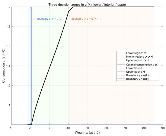
Figure 1. Three decision zones in the optimal consumption rule $c^{*}\left(x\right)$ under two–sided consumption constraints. The figure illustrates how the agent’s optimal consumption depends on initial wealth x at $t=0$. The solid black curve depicts the feedback policy $c^{*}\left(x\right)$, which can be divided into three regions: (i) Lower region ($c^{*}\left(x\right)=L$): when wealth is low, the lower bound L binds and the agent consumes the subsistence level. (ii) Interior region ($L<c^{*}\left(x\right)<H$): for intermediate wealth levels, consumption increases smoothly with wealth as both bounds are inactive. (iii) Upper region ($c^{*}\left(x\right)=H$): when wealth is sufficiently high, the upper bound H binds and additional wealth no longer raises consumption. The vertical blue and red lines correspond to the boundaries $y=u^{\prime }\left(L\right)$ and $y=u^{\prime }\left(H\right)$, respectively, separating the three decision zones. Economically, these boundaries represent threshold levels of the shadow price of wealth that trigger transitions between binding and non-binding consumption constraints.

This paper takes a different angle: we study a finite-horizon problem with both upper and lower consumption constraints in a complete diffusion market. A finite planning horizon matters for at least three reasons. First, the shadow price of wealth is time-varying as the horizon shortens, generating horizon effects in the optimal rules that are absent under stationarity. Second, bequest or terminal-wealth motives interact nontrivially with consumption caps and floors near the horizon. Third, empirical applications such as retirement planning or finite-lived institutions require explicit terminal conditions.

This paper addresses three interrelated questions. First, how do two-sided consumption bounds jointly shape the agent’s optimal consumption and portfolio rules within a finite horizon? Second, how does the time-varying shadow price of wealth $Y_t^{*}$ generate horizon effects that are absent in infinite-horizon or steady-state models? Third, can the dual-martingale approach yield tractable closed-form solutions even when both lower and upper consumption limits are imposed? We show that the answer to all three is affirmative.

Compared to the infinite-horizon analysis of Ma, Yi, and Guan [11], this paper provides a finite-horizon, closed-form dual characterization that explicitly captures time-dependent adjustments of the shadow price and constraint-binding probabilities. This formulation reveals how horizon effects, terminal-wealth considerations, and dual curvature jointly determine the geometry of optimal consumption and investment policies.

Methodologically, we adopt the dual-martingale method of [5,8] and subsequent convex duality refinements [15,16]. We construct the stochastic discount factor and the dual process, derive closed-form integral representations for the dual value function and its first two derivatives, and obtain feedback formulas for optimal consumption, portfolio, and wealth. These results yield a sharp economic picture: the optimal consumption rule is piecewise—it equals L at low wealth, follows the unconstrained Merton ratio in the interior, and is capped at H at high wealth—while the portfolio policy adjusts through the curvature of the dual value. The analysis parallels the classical complete-market martingale treatment [6,7,8] and connects to broader stochastic control references [9,10,19,20] as well as constraint-driven portfolio phenomena such as drawdown control [21]. Overall, the paper complements the infinite-horizon results in Ma, Yi, and Guan [11] by delivering a finite-horizon, closed-form dual characterization under explicit two-sided consumption bounds.

The remainder of this paper is organized as follows. Section 2 introduces the finite-horizon optimal consumption and investment problem under both upper and lower consumption constraints. Section 3 reformulates the problem via the dual-martingale approach and analyzes the properties of the resulting dual value function. Section 4 establishes the duality theorem and derives explicit expressions for the optimal strategies. Section 5 presents numerical illustrations that highlight the economic implications of the model. Finally, Section 6 concludes the paper.

2. Model

We consider a finitely lived agent who makes consumption and investment decisions over a fixed planning horizon $[0,T]$, where $T>0$ represents the terminal time, such as retirement or death. The economy is modeled in continuous time and assumed to be frictionless and complete. All sources of uncertainty are captured on a filtered probability space $(\mathrm{\Omega },\mathcal{F},\mathbb{F},\mathbb{P})$, where $\mathbb{F}:={\left({\mathcal{F}}_t\right)}_{t\in [0,T]}$ is the augmented filtration generated by a standard Brownian motion ${\left(B_t\right)}_{t\in [0,T]}$ satisfying the usual conditions.

(i)

Risk-free asset. The first asset is a risk-free bond (or bank account) that grows at a constant rate of return $r>0$:

$$d{B}_t=r{B}_{t}dt,B_0=1.$$

This asset provides a safe investment opportunity with a deterministic return and serves as the numéraire in the economy.

(ii)

Risky asset. The second asset is a risky stock whose price follows a geometric Brownian motion:

$${\displaystyle \frac{d{S}_t}{S_t}}=\mu dt+\sigma d{B}_t,$$

where $\mu >r$ denotes the expected rate of return and $\sigma >0$ is the volatility. The excess return $\mu -r$ represents the risk premium earned by holding the risky asset.

The agent starts with an initial wealth $x>0$ at time $t=0$ and chooses two progressively measurable processes: the consumption rate $c_t$ and the amount ${\pi }_t$ invested in the risky asset. The remainder $X_t^{c,\pi }-{\pi }_t$ is invested in the risk-free asset. The wealth dynamics are given by

$$d{X}_t^{c,\pi }=\left(r{X}_t^{c,\pi }+{\pi }_t(\mu -r)-c_t\right)dt+{\pi }_t\sigma d{B}_t,X_0^{c,\pi }=x>0.$$

(1)

The first term in the drift represents the risk-free accumulation of wealth, while the second term captures the expected excess gain from risky investment. The diffusion term ${\pi }_t\sigma d{B}_t$ reflects stochastic fluctuations in wealth due to market uncertainty.

• Consumption constraints. At each time $t\in [0,T]$, consumption must satisfy the following bounds:

$$L\le c_t\le H,\forall t\in [0,T],$$

(2)

where $0<L<H$. The lower bound L represents a subsistence level below which the agent cannot sustain a minimal standard of living, while the upper bound H captures an institutional or behavioral limit—such as liquidity constraints or physical saturation of consumption. These bounds ensure that consumption remains economically feasible throughout the planning horizon.

• Preferences and objective. The agent derives utility from both consumption during life and residual wealth at the terminal time. The expected lifetime utility is defined by

$$\mathfrak{U}(x;c,\pi ):=\mathbb{E}\left[{\int }_0^T{e}^{-\beta t}u\left(c_t\right)dt+e^{-\beta T}{U}_B\left(X_T^{c,\pi }\right)\right],$$

(3)

where $\beta >0$ is the subjective discount rate. The instantaneous utility from consumption $u(·)$ and the utility from terminal wealth $U_B(·)$ are both assumed to be of the constant relative risk aversion (CRRA) type:

$$u\left(c\right)={\displaystyle \frac{c^{1-\gamma }}{1-\gamma }},U_B\left(x\right)=u\left(k_{B}x\right)={\displaystyle \frac{{\left(k_{B}x\right)}^{1-\gamma }}{1-\gamma }},$$

(4)

where $\gamma >0$, $\gamma \ne 1$, is the relative risk aversion coefficient and $k_B>0$ is a bequest intensity parameter. The CRRA specification implies that the agent’s relative attitude toward risk is independent of wealth, which is a common and tractable assumption in intertemporal consumption models.

The assumption of a complete financial market is standard in continuous-time portfolio theory and enables the dual-martingale formulation to yield tractable closed-form solutions. The CRRA specification ensures homothetic preferences and facilitates explicit dual relationships between the value and policy functions. Moreover, the use of deterministic parameters $(r,\mu ,\sigma )$ isolates the effects of consumption constraints and horizon dependence from exogenous market uncertainty. While these assumptions enhance analytical transparency, they also limit the model’s scope: relaxing market completeness, introducing stochastic investment opportunities, or allowing for heterogeneous or non-separable preferences would generate richer but less tractable dynamics. We discuss such potential extensions in the Conclusion.

• Admissible strategies. For a given initial wealth $x>0$, the set of admissible consumption–investment strategies is defined as

$$\begin{array}{cc}\hfill \mathcal{A}\left(x\right):=\left\{{(c_t,{\pi }_t)}_{t\in [0,T]}\right|& (c_t,{\pi }_t)\mathrm{are}\mathbb{F}\text{-}\mathrm{progressively}\mathrm{measurable},\hfill \\ \hfill & L\le c_t\le H,\forall t\in [0,T],\hfill \\ \hfill & X_t^{c,\pi }\ge 0\mathrm{a}.\mathrm{s}.\mathrm{for}\mathrm{all}t\in [0,T],\hfill \\ \hfill & \mathbb{E}\left[{\int }_0^T{e}^{-\beta t}{u}^{+}\left(c_t\right)dt+e^{-\beta T}{U}_B^{+}\left(X_T^{c,\pi }\right)\right]<\infty \},\hfill \end{array}$$

(5)

where $u^{+}$ and $U_B^{+}$ denote the positive parts of the respective utility functions. This definition guarantees that the consumption process and corresponding wealth trajectory are economically meaningful and mathematically well defined.

Problem 1.

For a given initial wealth $x>0$, the agent’s problem is to maximize the expected lifetime utility:

$$V\left(x\right):=\underset{(c,\pi )\in \mathcal{A}\left(x\right)}{\sup }\mathfrak{U}(x;c,\pi ).$$

(6)

The function $V\left(x\right)$ represents the agent’s value function, summarizing the maximal attainable utility given initial wealth x.

3. Optimization Problem

3.1. Dual-Martingale Approach

In this section, we reformulate the agent’s optimization problem using the dual-martingale approach. This method transforms the original dynamic control problem into a static convex optimization problem by introducing the market’s pricing kernel. Economically, it reflects the fundamental idea that all feasible consumption and investment plans must satisfy a single intertemporal budget constraint valued under the market’s state-price density. The dual-martingale approach evaluates any feasible plan by its market value: it replaces a sequence of dynamic trades with a single, priced “budget identity,” which makes the role of discounting and risk adjustment economically transparent. In this framework, the Lagrange multiplier y represents the shadow value of initial wealth—the marginal utility of relaxing the lifetime budget constraint—while the dual process $Y_t^y=y{e}^{\beta t}{H}_t$ traces how this shadow price evolves over time under market risk and subjective discounting. This interpretation links the mathematical dual problem to the economic trade-off between present consumption, future saving, and exposure to risk. Figure 2 illustrates the flow of the dual approach employed in this paper.

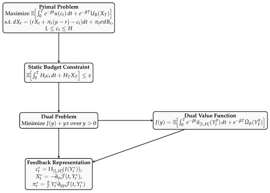
Figure 2. Flow of the dual-martingale approach. Starting from the primal stochastic control problem, the state-price density $H_t$ collapses intertemporal constraints into a single static budget. Introducing the Lagrange multiplier y leads to the dual problem, whose value function $J\left(y\right)$ admits an integral representation via the dual process $Y_t^y=y{e}^{\beta t}{H}_t$. The differentiation of $\mathcal{J}(t,y)$ provides the feedback formulas for optimal consumption, portfolio, and wealth.

• Market price of risk and state-price density. The key quantity governing the risk–return trade-off in the financial market is the market price of risk, which is defined as

$$\theta :={\displaystyle \frac{\mu -r}{\sigma }}.$$

It measures the excess expected return per unit of risk. Based on $\theta$, we define the state-price density (also known as the stochastic discount factor) ${\left(H_t\right)}_{t\in [0,T]}$ by

$$H_t:=\exp \left(-rt-\theta B_t-\frac{1}{2}{\theta }^{2}t\right),H_0=1.$$

(7)

The process $H_t$ discounts future random payoffs to their present value under the physical measure $\mathbb{P}$. When used as a Radon–Nikodym derivative, it converts $\mathbb{P}$ into the risk-neutral measure, under which discounted asset prices evolve as martingales. $H_t$ tells what one unit of cash at time t is worth today after adjusting for time and risk; movements in $H_t$ therefore govern how rapidly marginal values change along the horizon.

• Static budget constraint. For any admissible consumption–investment pair $(c_t,{\pi }_t)$, the wealth process (1) implies that

$$H_t{X}_t^{c,\pi }+{\int }_0^t{H}_s{c}_{s}ds$$

is a supermartingale. Taking expectations and using $H_0=1$, we obtain the static budget constraint

$$\mathbb{E}\left[{\int }_0^T{H}_t{c}_{t}dt+H_T{X}_T^{c,\pi }\right]\le x.$$

(8)

This condition summarizes all intertemporal trading restrictions into a single feasibility constraint: the present value of lifetime consumption and terminal wealth, evaluated at market prices, cannot exceed initial wealth. Intuitively, the inequality captures the fact that no investment strategy can finance more than the current endowment once adjusted for time and risk. Equation (8) is the lifetime budget: any admissible plan must “pay for itself” at market prices. It collapses dynamic rebalancing into one present-value check.

• Lagrangian and dual process. To incorporate the budget constraint into the objective function, we introduce a Lagrange multiplier $y>0$, which represents the shadow price of wealth or the agent’s marginal utility of relaxing the budget constraint. Define the dual process ${\left(Y_t^y\right)}_{t\in [0,T]}$ as

$$Y_t^y:=y{e}^{\beta t}{H}_t,t\in [0,T].$$

(9)

The exponential term $e^{\beta t}$ adjusts for the agent’s subjective discounting, while $H_t$ incorporates both time and risk adjustment. Economically, $Y_t^y$ can be viewed as the marginal utility-weighted price of consumption at time t. y is the shadow value of relaxing the initial budget by one unit; $Y_t^y$ tracks how that marginal value evolves with discounting and risk pricing, and thus it “prices” consumption at each date in marginal-utility units.

The Lagrangian functional is then written as

$$\begin{array}{cc}\hfill \mathcal{L}(c,\pi ,X_T;y)& =\mathbb{E}\left[{\int }_0^T{e}^{-\beta t}\left(u\left(c_t\right)-Y_t^y{c}_t\right)dt+e^{-\beta T}\left(U_B\left(X_T\right)-Y_T^y{X}_T\right)\right]+yx.\hfill \end{array}$$

(10)

The term $yx$ ensures that at the optimum, the Lagrange multiplier adjusts so that the budget constraint binds with equality. For each fixed $y>0$, maximizing $\mathcal{L}$ over $(c_t,X_T)$ leads to the first-order optimality conditions characterizing the dual relationship between utility and its convex conjugate.

• Reading the Lagrangian. The integrand $u\left(c_t\right)-Y_t^y{c}_t$ trades off marginal utility against its dual cost; optimality sets these equal in the interior and triggers corners when bounds bind.
• First-order conditions with consumption bounds. Given $y>0$, the optimal consumption $c_t^{*}\left(y\right)$ satisfies the Kuhn–Tucker system

$$e^{-\beta t}{u}^{\prime }\left(c_t^{*}\right)-y{H}_t\left\{\begin{array}{cc}=0,\hfill & \mathrm{if}L<c_t^{*}<H,\hfill \\ \le 0,\hfill & \mathrm{if}{c}_t^{*}=L,\hfill \\ \ge 0,\hfill & \mathrm{if}{c}_t^{*}=H.\hfill \end{array}\right.$$

Equivalently,

$$u^{\prime }\left(c_t^{*}\right)\left\{\begin{array}{cc}=Y_t^y,\hfill & \mathrm{if}L<c_t^{*}<H,\hfill \\ \ge Y_t^y,\hfill & \mathrm{if}{c}_t^{*}=L,\hfill \\ \le Y_t^y,\hfill & \mathrm{if}{c}_t^{*}=H.\hfill \end{array}\right.$$

Let $I={\left(u^{\prime }\right)}^{-1}$ denote the inverse of the marginal utility. The optimal consumption process is therefore given by the truncated policy

$$c_t^{*}\left(y\right)={\mathrm{\Pi }}_{[L,H]}\left(I\left(Y_t^y\right)\right)=\min \left\{\max \{I\left(Y_t^y\right),L\},H\right\},t\in [0,T],$$

(11)

where ${\mathrm{\Pi }}_{[L,H]}$ denotes the projection onto $[L,H]$. This projection captures the economic impact of the upper and lower consumption constraints: when the unconstrained optimal consumption $I\left(Y_t^y\right)$ exceeds H (or falls below L), the agent consumes exactly at the boundary, reflecting either saturation or subsistence behavior. Within the interior $(L,H)$, the agent behaves like the unconstrained Merton investor; outside, the rule sticks to L or H, which explains the three-zone policy used later in the numerical section.

Similarly, optimizing with respect to $X_T$ yields the terminal first–order condition

$$e^{-\beta T}{U}_B^{\prime }\left(X_T^{*}\right)-y{H}_T=0⟺U_B^{\prime }\left(X_T^{*}\right)=Y_T^y,$$

which implies

$$X_T^{*}\left(y\right)={\left(U_B^{\prime }\right)}^{-1}\left(Y_T^y\right).$$

(12)

This condition balances the marginal utility of terminal wealth with its shadow price, determining the optimal trade-off between lifetime consumption and bequest. The bequest choice equates the marginal utility of wealth at T with its dual price $Y_T^y$; a stronger bequest weight shifts optimal terminal wealth upward for a given y.

• CRRA specialization. Under the CRRA specification

$$u\left(c\right)={\displaystyle \frac{c^{1-\gamma }}{1-\gamma }},U_B\left(x\right)={\displaystyle \frac{{\left(k_{B}x\right)}^{1-\gamma }}{1-\gamma }},\gamma >0,\gamma \ne 1,$$

we have $u^{\prime }\left(c\right)=c^{-\gamma }$, $I\left(z\right)=z^{-1/\gamma }$, and ${\left(U_B^{\prime }\right)}^{-1}\left(z\right)=k_B^{(1-\gamma )/\gamma }{z}^{-1/\gamma }$. Consequently, the optimal consumption and terminal wealth policies are expressed as

$$c_t^{*}\left(y\right)={\mathrm{\Pi }}_{[L,H]}\left({\left(Y_t^y\right)}^{-1/\gamma }\right),X_T^{*}\left(y\right)=k_B^{(1-\gamma )/\gamma }{\left(Y_T^y\right)}^{-1/\gamma }.$$

(13)

The multiplier y scales the entire consumption–wealth plan, while the projection operator ensures that consumption respects both subsistence and satiation limits. Under CRRA, $Y_t^y$ maps one-to-one into interior consumption via ${\left(Y_t^y\right)}^{-1/\gamma }$; hence, movements in $Y_t^y$ directly translate into shifts across the three regions.

• Dual value function. To characterize the dual problem, define the convex conjugates of u and $U_B$ as

$${\tilde{u}}_{[L,H]}\left(z\right):=\underset{L\le c\le H}{\sup }\{u\left(c\right)-zc\}=u\left({\mathrm{\Pi }}_{[L,H]}\left(I\left(z\right)\right)\right)-z{\mathrm{\Pi }}_{[L,H]}\left(I\left(z\right)\right),$$

and

$${\tilde{U}}_B\left(z\right):=\underset{x\ge 0}{\sup }\{U_B\left(x\right)-zx\}=U_B\left({\left(U_B^{\prime }\right)}^{-1}\left(z\right)\right)-z{\left(U_B^{\prime }\right)}^{-1}\left(z\right).$$

Problem 2

(Dual Problem). Substituting the optimal policies (11) and (12) into the Lagrangian (10), and omitting the constant term $yx$, we define the dual value function as

$$J\left(y\right):=\mathbb{E}\left[{\int }_0^T{e}^{-\beta t}{\tilde{u}}_{[L,H]}\left(Y_t^y\right)dt+e^{-\beta T}{\tilde{U}}_B\left(Y_T^y\right)\right],y>0,$$

(14)

where ${\tilde{u}}_{[L,H]}$ and ${\tilde{U}}_B$ denote the convex conjugates of u and $U_B$, respectively. The function $J\left(y\right)$ is convex in y and represents the minimum attainable dual cost associated with the shadow price y.

Remark 1.

$J\left(y\right)$ aggregates three economic pieces: lower-bound spending at L, interior spending governed by $I(·)$, and upper-bound spending at H, plus the terminal bequest. In Section 4, ${\partial }_y\mathcal{J}$ and ${\partial }_{yy}\mathcal{J}$ will feed directly into wealth and risky demand via the feedback rules.

Accordingly, the dual optimization problem is given by

$$\underset{y>0}{\inf }\left(J\left(y\right)+yx\right),$$

(15)

where the optimal Lagrange multiplier $y^{*}$ determines the marginal utility value of initial wealth. It is straightforward to see that the following weak duality relation holds directly from the Lagrangian:

$$V\left(x\right)\le \underset{y>0}{\inf }\left(J\left(y\right)+yx\right).$$

(16)

We will later prove that the inequality in (16) actually holds with equality, thereby establishing that the primal value function $V\left(x\right)$ coincides with the right-hand side and that the envelope condition $x=-J^{\prime }\left(y^{*}\right)$ characterizes the primal–dual correspondence.

Remark 2

(Explicit form of the convex conjugates). For completeness, we provide the explicit expressions of ${\tilde{u}}_{[L,H]}\left(z\right)$ and ${\tilde{U}}_B\left(z\right)$ appearing in (14). For any $z>0$,

$${\tilde{u}}_{[L,H]}\left(z\right):=\underset{L\le c\le H}{\sup }\{u\left(c\right)-zc\}=\left\{\begin{array}{cc}u\left(H\right)-zH,\hfill & \mathrm{if}z<u^{\prime }\left(H\right),\hfill \\ u\left({\left(u^{\prime }\right)}^{-1}\left(z\right)\right)-z{\left(u^{\prime }\right)}^{-1}\left(z\right),\hfill & \mathrm{if}{u}^{\prime }\left(H\right)\le z\le u^{\prime }\left(L\right),\hfill \\ u\left(L\right)-zL,\hfill & \mathrm{if}z>u^{\prime }\left(L\right),\hfill \end{array}\right.$$

(17)

and

$${\tilde{U}}_B\left(z\right):=\underset{x\ge 0}{\sup }\{U_B\left(x\right)-zx\}=U_B\left({\left(U_B^{\prime }\right)}^{-1}\left(z\right)\right)-z{\left(U_B^{\prime }\right)}^{-1}\left(z\right).$$

(18)

Under the CRRA specification (4), we have $u^{\prime }\left(c\right)=c^{-\gamma }$ and $U_B^{\prime }\left(x\right)=k_B^{1-\gamma }{x}^{-\gamma }$, leading to

$$\begin{array}{cc}\hfill {\tilde{u}}_{[L,H]}\left(z\right)& =\left\{\begin{array}{cc}{\displaystyle \frac{H^{1-\gamma }}{1-\gamma }-zH,}\hfill & \mathit{if}z<H^{-\gamma },\hfill \\ {\displaystyle \frac{\gamma }{1-\gamma }{z}^{1-1/\gamma },}\hfill & \mathit{if}{H}^{-\gamma }\le z\le L^{-\gamma },\hfill \\ {\displaystyle \frac{L^{1-\gamma }}{1-\gamma }-zL,}\hfill & \mathit{if}z>L^{-\gamma },\hfill \end{array}\right.\hfill \\ \hfill {\tilde{U}}_B\left(z\right)& ={\displaystyle \frac{\gamma }{1-\gamma }}{k}_B^{{\displaystyle \frac{1-\gamma }{\gamma }}}{z}^{1-1/\gamma }.\hfill \end{array}$$

(19)

These piecewise expressions clearly illustrate the effect of the upper and lower consumption bounds on the shape of the dual functions.

3.2. Derivation of Explicit-Form for $J\left(y\right)$

To analyze the dual problem in a time-consistent way, we introduce the time-t version of the dual value function. Let ${\mathbb{E}}_t[·]:=\mathbb{E}[·|{\mathcal{F}}_t]$ denote conditional expectation and recall the state-price density H in (7). For each $t\in [0,T]$ and $y>0$, define

$$\mathcal{J}(t,y):={\mathbb{E}}_t\left[{\int }_t^T{e}^{-\beta (s-t)}{\tilde{u}}_{[L,H]}\left(Y_s^{t,y}\right)ds+e^{-\beta (T-t)}{\tilde{U}}_B\left(Y_T^{t,y}\right)\right],$$

(20)

$\mathcal{J}(t,y)$ is the dual cost-to-go at time t: it prices, in marginal-utility units, the remaining lifetime consumption and the terminal bequest under the shadow price y. A lower (higher) y relaxes (tightens) the intertemporal budget and thus lowers (raises) the dual cost. Here, the time-t dual process ${\left(Y_s^{t,y}\right)}_{s\in [t,T]}$ is given by

$$Y_s^{t,y}:=y{e}^{\beta (s-t)}{\displaystyle \frac{H_s}{H_t}},s\in [t,T],Y_t^{t,y}=y.$$

(21)

$Y_s^{t,y}$ is the shadow price of one unit of consumption at s, which is expressed in time-t marginal-utility units. Its movements combine pure time preference $e^{\beta (s-t)}$ and market pricing via $H_s/H_t$. By construction, $\mathcal{J}(0,y)=J\left(y\right)$ in (14).

Equivalent Representations

Using the explicit form of H,

$${\displaystyle \frac{H_s}{H_t}}=\exp \left(-r(s-t)-\theta (B_s-B_t)-\frac{1}{2}{\theta }^2(s-t)\right),$$

we may write

$$Y_s^{t,y}=y\exp \left((\beta -r)(s-t)-\theta (B_s-B_t)-\frac{1}{2}{\theta }^2(s-t)\right),s\in [t,T].$$

(22)

Equivalently, $Y^{t,y}$ solves the linear SDE

$$d{Y}_s^{t,y}=Y_s^{t,y}\left((\beta -r)ds-\theta d{B}_s\right),Y_t^{t,y}=y,$$

(23)

so that $\log Y_s^{t,y}$ is (conditionally) Gaussian given ${\mathcal{F}}_t$. When $\beta >r$, the drift $(\beta -r)$ pushes $Y^{t,y}$ up on average (consumption becomes relatively more “expensive” in dual units as time passes), while the term $-\theta d{B}_s$ propagates market risk into the shadow price. The factor $e^{\beta (s-t)}$ adjusts for time preference while the ratio $H_s/H_t$ prices risk and time between t and s. Hence, $Y_s^{t,y}$ is the shadow price of one unit of consumption at s, which is expressed in marginal-utility units at time t when the Lagrange multiplier equals y at t. The functional $\mathcal{J}(t,y)$ in (20) is the dual cost-to-go: it is the conditional dual value at time t, and its time-0 value coincides with the dual value function $J\left(y\right)$.

The next lemma converts this economic description into a normal-form integral for $\mathcal{J}(t,y)$ by exploiting the lognormality of $Y^{t,y}$.

Lemma 1.

The conditional dual value function $\mathcal{J}(t,y)$ admits the expression

$$\begin{array}{cc}\hfill \mathcal{J}(t,y)=& u\left(L\right){\int }_t^T{e}^{-\beta (s-t)}\mathbf{N}\left(d_0\left(s-t,{\displaystyle \frac{y}{u^{\prime }\left(L\right)}}\right)\right)ds-Ly{\int }_t^T{e}^{-r(s-t)}\mathbf{N}\left(d_1\left(s-t,{\displaystyle \frac{y}{u^{\prime }\left(L\right)}}\right)\right)ds\hfill \\ \hfill & +{\displaystyle \frac{\gamma }{1-\gamma }}{y}^{1-{\displaystyle \frac{1}{\gamma }}}{\int }_t^T{e}^{-K(s-t)}\mathbf{N}\left(d_{-\frac{1-\gamma }{\gamma }}\left(s-t,\frac{y}{u^{\prime }\left(H\right)}\right)\right)ds\hfill \\ \hfill & -\frac{\gamma }{1-\gamma }{y}^{1-\frac{1}{\gamma }}{\int }_t^T{e}^{-K(s-t)}\mathbf{N}\left(d_{-\frac{1-\gamma }{\gamma }}\left(s-t,\frac{y}{u^{\prime }\left(L\right)}\right)\right)ds\hfill \\ \hfill & +u\left(H\right){\int }_t^T{e}^{-\beta (s-t)}\mathbf{N}\left(-d_0\left(s-t,\frac{y}{u^{\prime }\left(H\right)}\right)\right)ds-Hy{\int }_t^T{e}^{-r(s-t)}\mathbf{N}\left(-d_1\left(s-t,\frac{y}{u^{\prime }\left(H\right)}\right)\right)ds\hfill \\ \hfill & +e^{-K(T-t)}\frac{\gamma }{1-\gamma }{k}_B^{\frac{1-\gamma }{\gamma }}{y}^{1-{\displaystyle \frac{1}{\gamma }}},\hfill \end{array}$$

where $K:=r+{\displaystyle \frac{\beta -r}{\gamma }}+{\displaystyle \frac{\gamma -1}{{\gamma }^2}}{\displaystyle \frac{{\theta }^2}{2}}$ and $\mathbf{N}(·)$ is the cdf of a standard normal random variable, and

$$d_{\vartheta }\left(t,z\right):={\displaystyle \frac{\log z+(\beta -r-\frac{{\theta }^2}{2}+\vartheta {\theta }^2)t}{\theta \sqrt{t}}}.$$

Each term corresponds to one of the three consumption regions (lower L, interior, upper H) plus the bequest term. The Gaussian cdf $\mathbf{N}(·)$ gives the time-t probability that the shadow price falls in each region over $[t,T]$.

Remark 3.

The parameter K acts as an effective discount rate in the dual space, combining the subjective time preference β, the opportunity cost of capital r, and the risk–curvature adjustment term from the CRRA specification.

Proof. 

By (A.6)–(A.7) in Jeon and Oh [22], for any $\vartheta \in \mathbb{R}$ and $m>0$,

$$\begin{array}{cc}\hfill \mathbb{E}\left[{\left({\mathcal{Y}}_s^{t,y}\right)}^{\vartheta }{\mathbf{1}}_{\{{\mathcal{Y}}_s^{t,y}>m\}}\mid {\mathcal{F}}_t\right]& =y^{\vartheta }\exp \left(\left(\vartheta (\beta -r)+\frac{{\theta }^2}{2}\vartheta (\vartheta -1)\right)(s-t)\right)\mathbf{N}\left({\displaystyle \frac{\log \frac{y}{m}+(\beta -r-\vartheta \frac{{\theta }^2}{2}+\vartheta {\theta }^2)(s-t)}{\theta \sqrt{s-t}}}\right),\hfill \\ \hfill \mathbb{E}\left[{\left({\mathcal{Y}}_s^{t,y}\right)}^{\vartheta }{\mathbf{1}}_{\{{\mathcal{Y}}_s^{t,y}<m\}}\mid {\mathcal{F}}_t\right]& =y^{\vartheta }\exp \left(\left(\vartheta (\beta -r)+\frac{{\theta }^2}{2}\vartheta (\vartheta -1)\right)(s-t)\right)\mathbf{N}\left(-{\displaystyle \frac{\log \frac{y}{m}+(\beta -r-\vartheta \frac{{\theta }^2}{2}+\vartheta {\theta }^2)(s-t)}{\theta \sqrt{s-t}}}\right).\hfill \end{array}$$

(24)

Since

$$\begin{array}{cc}\hfill \mathcal{J}(t,y)& =\mathbb{E}\left[{\int }_t^T{e}^{-\beta (s-t)}{\tilde{u}}_{[L,H]}\left({\mathcal{Y}}_s^{t,y}\right)ds|{\mathcal{F}}_t\right]\hfill \\ & ={\int }_t^T{e}^{-\beta (s-t)}\mathbb{E}\left[(u\left(L\right)-L{\mathcal{Y}}_s^{t,y}){\mathbf{1}}_{\{{\mathcal{Y}}_s^{t,y}\ge u^{\prime }\left(L\right)\}}|{\mathcal{F}}_t\right]ds\hfill \\ & +{\int }_t^T{e}^{-\beta (s-t)}{\displaystyle \frac{\gamma }{1-\gamma }}\mathbb{E}\left[{\left({\mathcal{Y}}_s^{t,y}\right)}^{1-{\displaystyle \frac{1}{\gamma }}}{\mathbf{1}}_{\{u^{\prime }\left(H\right)<{\mathcal{Y}}_s^{t,y}<u^{\prime }\left(L\right)\}}|{\mathcal{F}}_t\right]ds\hfill \\ & +{\int }_t^T{e}^{-\beta (s-t)}\mathbb{E}\left[(u\left(H\right)-H{\mathcal{Y}}_s^{t,y}){\mathbf{1}}_{\{{\mathcal{Y}}_s^{t,y}<u^{\prime }\left(H\right)\}}|{\mathcal{F}}_t\right]ds\hfill \\ & +e^{-K(T-t)}\frac{\gamma }{1-\gamma }{k}_B^{\frac{1-\gamma }{\gamma }}{y}^{1-\frac{1}{\gamma }},\hfill \end{array}$$

the stated formula follows from (24) with $m=u^{\prime }\left(L\right)$ and $m=u^{\prime }\left(H\right)$. □

We recall the conditional dual value

$$\mathcal{J}(t,y)={\mathbb{E}}_t\left[{\int }_t^T{e}^{-\beta (s-t)}{\tilde{u}}_{[L,H]}\left(Y_s^{t,y}\right)ds+e^{-\beta (T-t)}{\tilde{U}}_B\left(Y_T^{t,y}\right)\right],Y_s^{t,y}=y{e}^{\beta (s-t)}{\displaystyle \frac{H_s}{H_t}}.$$

Later, we use ${\partial }_y\mathcal{J}$ and ${\partial }_{yy}\mathcal{J}$ to obtain wealth and risky demand via feedback formulas; the integrals above are therefore the primitive objects behind the policy curvature.

Lemma 2

(Regularity). Under the standing assumptions on $u,U_B$ and admissibility, the mapping $(t,y)\mapsto \mathcal{J}(t,y)$ belongs to $C^{1,2}\left([0,T)\times (0,\infty )\right)$.

Proof. 

From Lemma 1, the function $\mathcal{J}(t,y)$ is a finite linear combination of terms of the form

$${\int }_t^T{e}^{-\lambda (s-t)}F\left(d_{\vartheta }(s-t,y/m)\right)G\left(y\right)ds,$$

where $\lambda \in \{\beta ,r,K\}$, $m\in \{u^{\prime }\left(L\right),u^{\prime }\left(H\right)\}$, $\vartheta \in \{0,1,-\frac{1-\gamma }{\gamma }\}$, F is either $\mathbf{N}$ or $\mathbf{N}\circ (-\mathrm{id})$, and $G\left(y\right)\in \{1,y,y^{1-1/\gamma }\}$. Here,

$$d_{\vartheta }(\tau ,z)={\displaystyle \frac{\log z+(\beta -r-\frac{{\theta }^2}{2}+\vartheta {\theta }^2)\tau }{\theta \sqrt{\tau }}},\tau =s-t>0,z=y/m.$$

We verify differentiability in t and twice in y by differentiating under the integral sign, using the dominated convergence theorem.

• Dependence on y. Fix $(t,y)$. Since $\mathbf{N}$ is $C^{\infty }$ and ${\mathbf{N}}^{\prime }=\phi$ (the standard normal density), the chain rule gives

$${\partial }_{y}F\left(d_{\vartheta }\right)=F^{\prime }\left(d_{\vartheta }\right){\partial }_y{d}_{\vartheta }=\phi \left(d_{\vartheta }\right){\displaystyle \frac{1}{y\theta \sqrt{\tau }}},{\partial }_{yy}F\left(d_{\vartheta }\right)=\left(-d_{\vartheta }\phi \left(d_{\vartheta }\right)\right){\displaystyle \frac{1}{y^2{\theta }^2\tau }}-\phi \left(d_{\vartheta }\right){\displaystyle \frac{1}{y^2\theta \sqrt{\tau }}}.$$

Hence, for suitable constants $C_1,C_2>0$,

$$|{\partial }_{y}F\left(d_{\vartheta }\right)|\le {\displaystyle \frac{C_1}{y\sqrt{\tau }}},|{\partial }_{yy}F\left(d_{\vartheta }\right)|\le {\displaystyle \frac{C_2(1+|d_{\vartheta }|)}{y^2\tau }}.$$

The function $|d_{\vartheta }|\phi \left(d_{\vartheta }\right)$ is uniformly bounded for all $\tau >0$. As $\tau \downarrow 0$, either $d_{\vartheta }(\tau ,y/m)\to \pm \infty$, in which case $e^{-d_{\vartheta }^2/2}$ decays super-exponentially, or $d_{\vartheta }(\tau ,y/m)=O\left(\sqrt{\tau }\right)$ if $y/m\approx 1$, in which case $\phi \left(d_{\vartheta }\right)=O\left(1\right)$ and $d_{\vartheta }\phi \left(d_{\vartheta }\right)=O\left(\sqrt{\tau }\right)$. Thus, ${\partial }_{y}F$ behaves like ${\tau }^{-1/2}$ and ${\partial }_{yy}F$ like ${\tau }^{-1/2}$ near $\tau =0$, both of which are integrable because ${\int }_0^{\epsilon }{\tau }^{-1/2}d\tau <\infty$. Since $G\left(y\right)$ is $C^{\infty }$ on $(0,\infty )$, products with G and its derivatives preserve integrability. Therefore, differentiation with respect to y (and again with respect to y) can be interchanged with the integral, proving that $\mathcal{J}$ is twice continuously differentiable in y.

• Dependence on t. Differentiation in t involves three sources: (i) the exponential factor $e^{-\lambda (s-t)}$, (ii) the dependence of $d_{\vartheta }(s-t,y/m)$ on $\tau =s-t$, and (iii) the moving lower limit of integration. By the chain rule,

$${\partial }_{\tau }{d}_{\vartheta }(\tau ,y/m)={\displaystyle \frac{\beta -r-\frac{{\theta }^2}{2}+\vartheta {\theta }^2}{\theta \sqrt{\tau }}}-{\displaystyle \frac{\log (y/m)}{2\theta {\tau }^{3/2}}},$$

and hence

$${\partial }_{\tau }F\left(d_{\vartheta }\right)=\phi \left(d_{\vartheta }\right){\partial }_{\tau }{d}_{\vartheta }=\phi \left(d_{\vartheta }\right)\left(\mathcal{O}\left({\tau }^{-1/2}\right)+\mathcal{O}\left({\tau }^{-3/2}\right)\right).$$

The Gaussian factor $\phi \left(d_{\vartheta }\right)$ decays exponentially in $|d_{\vartheta }|$, ensuring integrability near $\tau =0$. The boundary term at $s=t$ arising from the Leibniz rule is finite because $\mathbf{N}\left(d_{\vartheta }(0^{+},y/m)\right)$ has a finite limit and the exponential factor equals 1 there. Thus, ${\partial }_t\mathcal{J}$ exists and is continuous.

Combining these arguments shows that ${\partial }_t\mathcal{J}$, ${\partial }_y\mathcal{J}$, and ${\partial }_{yy}\mathcal{J}$ all exist and are continuous on $[0,T)\times (0,\infty )$, proving that

$$\mathcal{J}\in C^{1,2}\left([0,T)\times (0,\infty )\right).$$

□

Regularity ensures that derivatives of $\mathcal{J}$ can be used safely as state-dependent policy objects in the feedback rules without invoking viscosity arguments.

Lemma 3

(Strict convexity in y). For each $t\in [0,T)$, the map $y\mapsto \mathcal{J}(t,y)$ is strictly convex on $(0,\infty )$.

Proof. 

Fix t and note $Y_s^{t,y}=y{\Xi }_{t,s}$ is affine in y. The compositions $y\mapsto {\tilde{u}}_{[L,H]}\left(y{\Xi }_{t,s}\right)$ are convex because ${\tilde{u}}_{[L,H]}$ is convex. Moreover, the terminal term $y\mapsto {\tilde{U}}_B\left(y{\Xi }_{t,T}\right)$ is strictly convex since ${\tilde{U}}_B$ is strictly convex (as the convex conjugate of a strictly concave $U_B$) and ${\Xi }_{t,T}>0$ a.s. Taking expectations and adding non-negative weights $e^{-\beta (·)}$ preserves (strict) convexity; thus, $\mathcal{J}(t,·)$ is strictly convex. □

Strict convexity in y implies a unique optimal multiplier $y^{*}$ for each x, hence a unique shadow price and, consequently, well-defined feedback policies.

Proposition 1

(First derivative in y). For $(t,y)\in [0,T)\times (0,\infty )$,

$${\partial }_y\mathcal{J}(t,y)={\mathbb{E}}_t\left[{\int }_t^T{e}^{-\beta (s-t)}{\tilde{u}}_{[L,H]}^{\prime }\left(Y_s^{t,y}\right){\displaystyle \frac{Y_s^{t,y}}{y}}ds+e^{-\beta (T-t)}{\tilde{U}}_B^{\prime }\left(Y_T^{t,y}\right){\displaystyle \frac{Y_T^{t,y}}{y}}\right].$$

(25)

Equivalently,

$$H_t\left(-{\partial }_y\mathcal{J}(t,y)\right)={\mathbb{E}}_t\left[{\int }_t^T{H}_s{c}^{*}\left(Y_s^{t,y}\right)ds+H_T{X}_T^{*}\left(Y_T^{t,y}\right)\right],$$

(26)

where $c^{*}\left(z\right):={\Pi }_{[L,H]}\left(I\left(z\right)\right)$, $X_T^{*}\left(z\right):={\left(U_B^{\prime }\right)}^{-1}\left(z\right)$, and $I={\left(u^{\prime }\right)}^{-1}$. In particular, under CRRA, $c^{*}\left(z\right)={\Pi }_{[L,H]}\left(z^{-1/\gamma }\right)$ and $X_T^{*}\left(z\right)=k_B^{{\displaystyle \frac{1-\gamma }{\gamma }}}{z}^{-1/\gamma }$.

Equation (26) links the dual slope $-{\partial }_y\mathcal{J}$ to the present value of optimal spending and bequest. Hence, $X_t^{*}$ and ${\pi }_t^{*}$ below inherit their shapes from the sign and curvature of ${\partial }_y\mathcal{J}$ and ${\partial }_{yy}\mathcal{J}$.

Proof. 

We recall that

$$\mathcal{J}(t,y)={\mathbb{E}}_t\left[{\int }_t^T{e}^{-\beta (s-t)}{\tilde{u}}_{[L,H]}\left(Y_s^{t,y}\right)ds+e^{-\beta (T-t)}{\tilde{U}}_B\left(Y_T^{t,y}\right)\right],Y_s^{t,y}=y{\Xi }_{t,s},$$

where ${\Xi }_{t,s}:=e^{\beta (s-t)}{H}_s/H_t>0$ is independent of y. To verify the differentiability of $\mathcal{J}(t,y)$ with respect to y, fix $ϵ>0$ and observe that $Y_s^{t,y\pm ϵ}=(y\pm ϵ){\Xi }_{t,s}=Y_s^{t,y}(1\pm ϵ/y)$. Hence, the difference quotient satisfies

$$\begin{array}{cc}\hfill {\displaystyle \frac{\mathcal{J}(t,y\pm ϵ)-\mathcal{J}(t,y)}{ϵ}}={\mathbb{E}}_t[& {\int }_t^T{e}^{-\beta (s-t)}{\displaystyle \frac{{\tilde{u}}_{[L,H]}\left(Y_s^{t,y}(1\pm \frac{ϵ}{y})\right)-{\tilde{u}}_{[L,H]}\left(Y_s^{t,y}\right)}{ϵ}}ds\hfill \\ & +e^{-\beta (T-t)}{\displaystyle \frac{{\tilde{U}}_B\left(Y_T^{t,y}(1\pm \frac{ϵ}{y})\right)-{\tilde{U}}_B\left(Y_T^{t,y}\right)}{ϵ}}].\hfill \end{array}$$

Both ${\tilde{u}}_{[L,H]}$ and ${\tilde{U}}_B$ are convex, locally Lipschitz, and piecewise $C^{\infty }$ with possible kinks only at $u^{\prime }\left(L\right)$ and $u^{\prime }\left(H\right)$. Since $Y_s^{t,y}$ has a continuous distribution, the events $\{Y_s^{t,y}=u^{\prime }\left(L\right)\}$ and $\{Y_s^{t,y}=u^{\prime }\left(H\right)\}$ occur with zero probability. Therefore, by the mean value theorem applied pointwise (off a null set) and by the dominated convergence theorem (using the admissibility conditions to guarantee integrability), the limit as $ϵ\downarrow 0$ can be passed inside both the conditional expectation and the time integral. Using ${\partial }_y{Y}_s^{t,y}=Y_s^{t,y}/y$ and the chain rule then gives

$${\partial }_y\mathcal{J}(t,y)={\mathbb{E}}_t\left[{\int }_t^T{e}^{-\beta (s-t)}{\tilde{u}}_{[L,H]}^{\prime }\left(Y_s^{t,y}\right){\displaystyle \frac{Y_s^{t,y}}{y}}ds+e^{-\beta (T-t)}{\tilde{U}}_B^{\prime }\left(Y_T^{t,y}\right){\displaystyle \frac{Y_T^{t,y}}{y}}\right],$$

which corresponds to (25).

Next, by convex conjugacy and the envelope theorem for the pointwise suprema that define ${\tilde{u}}_{[L,H]}$ and ${\tilde{U}}_B$, the derivatives satisfy ${\tilde{u}}_{[L,H]}^{\prime }\left(z\right)=-c^{*}\left(z\right)$ and ${\tilde{U}}_B^{\prime }\left(z\right)=-X_T^{*}\left(z\right)$ for almost every $z>0$, where $c^{*}\left(z\right)={\Pi }_{[L,H]}\left(I\left(z\right)\right)$ and $X_T^{*}\left(z\right)={\left(U_B^{\prime }\right)}^{-1}\left(z\right)$. Substituting these relations into the previous equation and multiplying both sides by $-y$ yields

$$-y{\partial }_y\mathcal{J}(t,y)={\mathbb{E}}_t\left[{\int }_t^T{e}^{-\beta (s-t)}{c}^{*}\left(Y_s^{t,y}\right)Y_s^{t,y}ds+e^{-\beta (T-t)}{X}_T^{*}\left(Y_T^{t,y}\right)Y_T^{t,y}\right],$$

which gives (26).

Finally, under CRRA preferences $u\left(c\right)={\displaystyle \frac{c^{1-\gamma }}{1-\gamma }}$ and $U_B\left(x\right)={\displaystyle \frac{{\left(k_{B}x\right)}^{1-\gamma }}{1-\gamma }}$ with $\gamma >0$, $\gamma \ne 1$, we have ${\left(u^{\prime }\right)}^{-1}\left(z\right)=z^{-1/\gamma }$ and ${\left(U_B^{\prime }\right)}^{-1}\left(z\right)=k_B^{(1-\gamma )/\gamma }{z}^{-1/\gamma }$. Therefore, $c^{*}\left(z\right)={\Pi }_{[L,H]}\left(z^{-1/\gamma }\right)$ and $X_T^{*}\left(z\right)=k_B^{(1-\gamma )/\gamma }{z}^{-1/\gamma }$, completing the proof. □

Lemma 4

(Normal-form integral representation of $y{\partial }_y\mathcal{J}(t,y)$). For $(t,y)\in [0,T)\times (0,\infty )$, the conditional dual value function $\mathcal{J}(t,y)$ satisfies

$$\begin{array}{cc}\hfill {\partial }_y\mathcal{J}(t,y)& ={\displaystyle \frac{1}{y}}{\mathbb{E}}_t\left[{\int }_t^T{e}^{-\beta (s-t)}{\tilde{u}}_{[L,H]}^{\prime }\left(Y_s^{t,y}\right)Y_s^{t,y}ds+e^{-\beta (T-t)}{\tilde{U}}_B^{\prime }\left(Y_T^{t,y}\right)Y_T^{t,y}\right]\hfill \\ \hfill & =-L{\int }_t^T{e}^{-r(s-t)}\mathbf{N}\left(d_1\left(s-t,{\displaystyle \frac{y}{u^{\prime }\left(L\right)}}\right)\right)ds\hfill \\ \hfill & -y^{-{\displaystyle \frac{1}{\gamma }}}{\int }_t^T{e}^{-K(s-t)}\left\{\mathbf{N}\left(d_{-{\displaystyle \frac{1-\gamma }{\gamma }}}\left(s-t,{\displaystyle \frac{y}{u^{\prime }\left(H\right)}}\right)\right)-\mathbf{N}\left(d_{-{\displaystyle \frac{1-\gamma }{\gamma }}}\left(s-t,\frac{y}{u^{\prime }\left(L\right)}\right)\right)\right\}ds\hfill \\ \hfill & -H{\int }_t^T{e}^{-r(s-t)}\mathbf{N}\left(-d_1\left(s-t,\frac{y}{u^{\prime }\left(H\right)}\right)\right)ds\hfill \\ \hfill & -e^{-K(T-t)}{k}_B^{\frac{1-\gamma }{\gamma }}{y}^{-\frac{1}{\gamma }}.\hfill \end{array}$$

(27)

• Intuition. The four lines correspond to (i) lower-region spending at L, (ii) interior spending, (iii) upper-region spending at H, and (iv) the bequest term. The normal cdfs encode the probabilities that $Y^{t,y}$ lies in each region over $[t,T]$, so the shape of ${\partial }_y\mathcal{J}$ is directly governed by how often constraints bind.

Proof. 

From

$$y{\partial }_y\mathcal{J}(t,y)={\mathbb{E}}_t\left[{\int }_t^T{e}^{-\beta (s-t)}{\tilde{u}}_{[L,H]}^{\prime }\left(Y_s^{t,y}\right)Y_s^{t,y}ds+e^{-\beta (T-t)}{\tilde{U}}_B^{\prime }\left(Y_T^{t,y}\right)Y_T^{t,y}\right]$$

and the conjugacy identities ${\tilde{u}}_{[L,H]}^{\prime }\left(z\right)=-c^{*}\left(z\right)$, ${\tilde{U}}_B^{\prime }\left(z\right)=-X_T^{*}\left(z\right)$, with

$$c^{*}\left(z\right)=\left\{\begin{array}{cc}L,\hfill & z\le u^{\prime }\left(L\right)(\mathrm{upper}\mathrm{region}),\hfill \\ z^{-1/\gamma },\hfill & u^{\prime }\left(H\right)\le z\le u^{\prime }\left(L\right)(\mathrm{middle}\mathrm{region}),\hfill \\ H,\hfill & z\le u^{\prime }\left(H\right)(\mathrm{lower}\mathrm{region}),\hfill \end{array}\right.X_T^{*}\left(z\right)=k_B^{{\displaystyle \frac{1-\gamma }{\gamma }}}{z}^{-1/\gamma },$$

we obtain three running terms and one terminal term involving ${\mathbb{E}}_t\left[Y_s^{t,y}{\mathbf{1}}_{\{Y_s^{t,y}\gtrless m\}}\right]$ and ${\mathbb{E}}_t\left[{\left(Y_s^{t,y}\right)}^{1-1/\gamma }{\mathbf{1}}_{\{m_1<Y_s^{t,y}<m_2\}}\right]$ with thresholds $m=u^{\prime }\left(L\right),u^{\prime }\left(H\right)$. Applying the lognormal moment formulas ((A.6)–(A.7) in Jeon and Oh [22]) yields the stated $\mathbf{N}\left(d_{\vartheta }\right)$ expressions and the factors $e^{-r(s-t)}$, $e^{-K(s-t)}$ and the terminal term $e^{-K(T-t)}{k}_B^{(1-\gamma )/\gamma }{y}^{1-1/\gamma }$. □

Using Lemma C.1 in [22], it follows directly from Lemma 4 that the following result holds.

Lemma 5.

For all $t\in [0,T]$, we have

$$\underset{y\to 0+}{\lim }{\partial }_y\mathcal{J}(t,y)=-\infty \mathit{and}\underset{y\to \infty }{\lim }{\partial }_y\mathcal{J}(t,y)=0.$$

When $y\downarrow 0$, the budget is very slack, so the marginal value of further relaxing it goes to $-\infty$ (the agent wants to spend more); as $y\uparrow \infty$, the budget is extremely tight, so the marginal gain from additional relaxation vanishes, driving ${\partial }_y\mathcal{J}\to 0$.

4. Optimal Strategy

In this section, we establish the duality theorem and derive the corresponding optimal strategies.

Theorem 1

(Duality and Feedback Representation). For each initial wealth $x>0$, there exists a unique $y^{*}>0$ such that

$$x=-J^{\prime }\left(y^{*}\right)=-{\partial }_y\mathcal{J}(0,y^{*}).$$

Define the dual process, optimal consumption, and optimal terminal wealth by

$$Y_t^{*}:=y^{*}{e}^{\beta t}{H}_t,c_t^{*}:=c^{*}\left(Y_t^{*}\right)={\Pi }_{[L,H]}\left(I\left(Y_t^{*}\right)\right),\mathfrak{B}:=X_T^{*}\left(Y_T^{*}\right)={\left(U_B^{\prime }\right)}^{-1}\left(Y_T^{*}\right).$$

Then, the following statements hold:

(i) 

The value function satisfies the duality relation

$$V\left(x\right)=\underset{y>0}{\inf }\left(J\left(y\right)+yx\right)=J\left(y^{*}\right)+y^{*}x.$$

(ii) 

The optimal pair $(c^{*},{\pi }^{*})$ is admissible and attains the supremum in the primal problem, i.e.,

$$V\left(x\right)=\mathfrak{U}(x;c^{*},{\pi }^{*}).$$

(iii) 

The corresponding wealth process admits the representation

$$X_t^{*}=-{\partial }_y\mathcal{J}(t,Y_t^{*}),{\pi }_t^{*}={\displaystyle \frac{\theta }{\sigma }}{Y}_t^{*}{\partial }_{yy}\mathcal{J}(t,Y_t^{*}).$$

The parameter $y^{*}$ serves as the shadow price of initial wealth, representing the marginal utility value of relaxing the static budget constraint (8). Economically, $y^{*}$ declines monotonically with wealth: a higher x lowers $y^{*}$ and thus relaxes the budget in dual units. Its dynamic counterpart, $Y_t^{*}=y^{*}{e}^{\beta t}{H}_t$, evolves jointly with subjective discounting and the state-price density, capturing how marginal utility is adjusted for time and risk. The feedback representation further clarifies this link: wealth and portfolio demand are governed by the level and curvature of the dual cost $\mathcal{J}$. Specifically, $X_t^{*}$ equals the negative slope $-{\partial }_y\mathcal{J}$, while risky exposure scales with $Y_t^{*}{\partial }_{yy}\mathcal{J}$.

Proof. 

By Lemmas 3 and 5, there exists a unique $y^{*}>0$ satisfying

$$x=-J^{\prime }\left(y^{*}\right)=-{\partial }_y\mathcal{J}(0,y^{*}).$$

Define $Y_t^{*}:=y^{*}{e}^{\beta t}{H}_t$, $c_t^{*}:=c^{*}\left(Y_t^{*}\right)$, and $\mathfrak{B}:=X_T^{*}\left(Y_T^{*}\right)$. Then, from Proposition 1 and the static budget identity, we obtain

$$x=\mathbb{E}\left[{\int }_0^T{H}_t{c}_t^{*}dt+H_T\mathfrak{B}\right].$$

(28)

By Theorem 3.5 in [8], there exists an admissible portfolio ${\pi }_t^{*}$ such that $(c^{*},{\pi }^{*})\in \mathcal{A}\left(x\right)$ and the corresponding wealth process $X_t^{*}:=X_t^{c^{*},{\pi }^{*}}$ satisfies $X_0^{*}=x$ and $X_T^{*}=\mathfrak{B}$. Moreover, the budget constraint implies

$$H_t{X}_t^{*}={\mathbb{E}}_t\left[{\int }_t^T{H}_s{c}_s^{*}ds+H_T\mathfrak{B}\right],$$

which in turn gives $X_t^{*}=-{\partial }_y\mathcal{J}(t,Y_t^{*})$.

Using this representation, we compute

$$\begin{array}{c}\hfill x{y}^{*}=y^{*}\mathbb{E}\left[{\int }_0^T{H}_t{c}_t^{*}dt+H_T\mathfrak{B}\right]=\mathbb{E}\left[{\int }_0^T{e}^{-\beta t}{Y}_t^{*}{c}_t^{*}dt+e^{-\beta T}{Y}_T^{*}\mathfrak{B}\right]=\mathfrak{U}(x;c^{*},{\pi }^{*})-J\left(y^{*}\right).\end{array}$$

(29)

This implies the chain of inequalities

$$V\left(x\right)\le \underset{y>0}{\inf }\left(J\left(y\right)+yx\right)\le J\left(y^{*}\right)+y^{*}x=\mathfrak{U}(x;c^{*},{\pi }^{*})\le V\left(x\right),$$

and hence,

$$V\left(x\right)=\underset{y>0}{\inf }\left(J\left(y\right)+yx\right)=J\left(y^{*}\right)+y^{*}x,$$

showing that $(c^{*},{\pi }^{*})$ is optimal.

Finally, differentiating $X_t^{*}=-{\partial }_y\mathcal{J}(t,Y_t^{*})$ with respect to t and applying Itô’s lemma gives

$$d{X}_t^{*}=\left(r{X}_t^{*}+{\pi }_t^{*}(\mu -r)-c_t^{*}\right)dt+{\pi }_t^{*}\sigma d{B}_t,$$

from which it follows that

$${\pi }_t^{*}={\displaystyle \frac{\theta }{\sigma }}{Y}_t^{*}{\partial }_{yy}\mathcal{J}(t,Y_t^{*}).$$

□

(i) If $Y_t^{*}$ spends more time above $u^{\prime }\left(L\right)$ (lower region), consumption sits at L and $-{\partial }_y\mathcal{J}$ flattens, compressing risky demand. (ii) If $Y_t^{*}$ often falls below $u^{\prime }\left(H\right)$ (upper region), consumption hits H; without a strong bequest motive, ${\partial }_{yy}\mathcal{J}$ shrinks and the risky position declines. (iii) Stronger bequest utility (smaller $k_B$) raises the terminal curvature term, sustaining ${\partial }_{yy}\mathcal{J}$ and keeping ${\pi }_t^{*}>0$ at high wealth.

Using the expression for ${\partial }_y\mathcal{J}(t,y)$ given in Lemma 4, we can easily obtain the following representation for ${\partial }_{yy}\mathcal{J}(t,y)$:

$$\begin{array}{cc}\hfill {\partial }_{yy}\mathcal{J}(t,y)& =-L{\int }_t^T{e}^{-r(s-t)}{\displaystyle \frac{\mathbf{n}\left(d_1\left(s-t,\frac{y}{u^{\prime }\left(L\right)}\right)\right)}{y\theta \sqrt{s-t}}}ds\hfill \\ \hfill & +\frac{1}{\gamma }{y}^{-1/\gamma -1}{\int }_t^T{e}^{-K(s-t)}\left\{\mathbf{N}\left(d_{-\frac{1-\gamma }{\gamma }}\left(s-t,\frac{y}{u^{\prime }\left(H\right)}\right)\right)-\mathbf{N}\left(d_{-\frac{1-\gamma }{\gamma }}\left(s-t,\frac{y}{u^{\prime }\left(L\right)}\right)\right)\right\}ds\hfill \\ \hfill & -y^{-1/\gamma -1}{\int }_t^T{e}^{-K(s-t)}\frac{\mathbf{n}\left(d_{-\frac{1-\gamma }{\gamma }}\left(s-t,\frac{y}{u^{\prime }\left(H\right)}\right)\right)-\mathbf{n}\left(d_{-\frac{1-\gamma }{\gamma }}\left(s-t,\frac{y}{u^{\prime }\left(L\right)}\right)\right)}{\theta \sqrt{s-t}}ds\hfill \\ \hfill & +H{\int }_t^T{e}^{-r(s-t)}\frac{\mathbf{n}\left(d_1\left(s-t,\frac{y}{u^{\prime }\left(H\right)}\right)\right)}{y\theta \sqrt{s-t}}ds+e^{-K(T-t)}\frac{1}{\gamma }{k}_B^{\frac{1-\gamma }{\gamma }}{y}^{-1/\gamma -1}.\hfill \end{array}$$

(30)

Here, $\mathbf{N}$ and $\mathbf{n}$ denote the standard normal cumulative distribution and probability density functions, respectively.

The first and fourth lines are boundary terms (at L and H) and depress curvature when constraints bind frequently; the second and terminal terms counteract this via interior consumption and bequest intensity. Thus, the sign/magnitude of ${\partial }_{yy}\mathcal{J}$ across wealth explains the inverted-U portfolio pattern in the weak-bequest case and its attenuation when the bequest motive strengthens.

Therefore, the expressions for ${\partial }_y\mathcal{J}(t,y)$ and ${\partial }_{yy}\mathcal{J}(t,y)$ allow us to explicitly compute, as functions of y, the optimal consumption $c^{*}$, the optimal investment ${\pi }^{*}$, and the corresponding wealth process $X^{*}$.

5. Numerical Results

In this section, we present numerical illustrations of the optimal strategies derived in the previous section. We adopt the following baseline parameter values throughout the analysis:

$$\beta =0.03,r=0.02,\mu =0.07,\sigma =0.20,\gamma =3.0,$$

$$L=0.8,H=2.0,T=30.0.$$

For the bequest utility weight, we consider two contrasting scenarios:

$$k_B=100(\mathrm{weak}\mathrm{bequest}\mathrm{motive}),k_B=0.1(\mathrm{strong}\mathrm{bequest}\mathrm{motive}).$$

Note that the strength of the bequest motive is inversely related to $k_B^{1-\gamma }$; that is, a smaller $k_B$ corresponds to a larger $k_B^{1-\gamma }$, implying a stronger incentive to leave terminal wealth.

The baseline parameters are chosen to reflect standard long-run market and preference inputs and to keep the numerical illustrations transparent. First, we set the discount rate to $\beta =0.03$ and the risk-free rate to $r=0.02$, which are commonly used annual values in continuous-time calibrations and are consistent with moderate time preference and low safe returns. For the risky asset, we take an expected return $\mu =0.07$ and volatility $\sigma =0.20$, delivering a market price of risk $\theta =(\mu -r)/\sigma =0.25$ that is neither trivial nor extreme and keeps portfolio sensitivities economically plausible. We adopt CRRA preferences with $\gamma =3$, which is a mid-range value widely used in the macro-finance literature that avoids knife-edge behavior while generating realistic precautionary motives. Regarding consumption bounds, we normalize the scale so that the lower bound $L=0.8$ captures subsistence or fixed living costs, and the upper bound $H=2.0$ represents liquidity, adjustment, or saturation limits. The horizon is set to $T=30$ years, which is a representative planning window for retirement and institutional spending applications. Finally, for the bequest intensity, we consider $k_B\in \{100,0.1\}$ to bracket weak and strong bequest motives; because the effective weight is proportional to $k_B^{1-\gamma }$ under CRRA, a smaller $k_B$ corresponds to a stronger bequest force. These choices yield interior solutions in unconstrained regions, activate both consumption bounds in relevant wealth ranges, and make horizon effects visible without relying on knife-edge parameters.

Under these baselines, consumption saturates at both bounds in the tails of wealth, while the risky position is hump-shaped in the weak-bequest case and remains positive at high wealth when the bequest motive is strong. These patterns align exactly with the curvature implications of ${\partial }_{yy}\mathcal{J}$ highlighted above.

• Consumption policy. The optimal consumption $c^{*}\left(y\right)$ behaves as expected under two-sided consumption constraints. When wealth is small, the lower bound binds, and the agent consumes at the subsistence level L. As wealth increases, consumption rises smoothly until the upper bound H is reached, after which it remains constant. This monotonic and bounded pattern contrasts with the unconstrained Merton rule, where consumption grows proportionally with wealth.
• Investment policy. Because the consumption behavior is straightforward under two-sided constraints, it is more instructive to analyze how the optimal investment (risky asset holding) varies with wealth. The risky position follows the feedback representation

  $${\pi }_t^{*}={\displaystyle \frac{\theta }{\sigma }}{Y}_t^{*}{\partial }_{yy}\mathcal{J}(t,Y_t^{*}),Y_t^{*}=y^{*}{e}^{\beta t}{H}_t,$$

  where $\theta =(\mu -r)/\sigma$. Figure 3 illustrates the relationship between the initial wealth $X_0^{*}$ and the optimal risky position ${\pi }_0^{*}$ under different strengths of the bequest motive.

Figure 3. Portfolio–wealth relation under two-sided consumption constraints. The risky position is computed from the feedback rule ${\displaystyle {\pi }_t^{*}=\frac{\theta }{\sigma }{Y}_t^{*}{\partial }_{yy}\mathcal{J}(t,Y_t^{*})}$ with $X_t^{*}=-{\partial }_y\mathcal{J}(t,Y_t^{*})$. Panel (a) (weak bequest): the curve exhibits an inverted-U shape and approaches zero at both ends. For low wealth, the lower consumption constraint L binds, reducing the marginal value of risk taking. For high wealth, the upper bound H binds and, without a strong bequest motive, the marginal utility of terminal wealth vanishes, again driving ${\pi }_t^{*}$ to zero. Panel (b) (strong bequest): a higher weight on terminal utility preserves positive marginal utility at high wealth levels, increasing ${\partial }_{yy}\mathcal{J}$ and thus sustaining a strictly positive risky position even for large $X_0^{*}$. Economically, the stronger bequest motive encourages the agent to maintain exposure to risky assets to accumulate and protect terminal wealth. (a) Optimal risky position ${\pi }_0^{*}$ as a function of wealth $X_0^{*}$ when the bequest weight is negligible ($k_B=100$). (b) Optimal risky position ${\pi }_0^{*}$ as a function of wealth $X_0^{*}$ when the bequest weight is strong ($k_B=0.1$).

The inverted-U pattern of the risky position can be understood through the behavior of the marginal value of wealth. When wealth is low, the lower consumption bound L binds, forcing the agent to consume at the subsistence level; since additional risk cannot meaningfully improve utility, the incentive to hold risky assets is weak. When wealth is high, the upper bound H becomes binding, so further increases in wealth no longer raise utility through higher consumption—producing a similar decline in risk taking. Risk exposure therefore peaks in the interior region where neither constraint is active, leading to the inverted-U shape. Over time, horizon effects arise because the shadow price $Y_t^{*}$ becomes more sensitive as t approaches T: as the horizon shortens, the agent reduces risky exposure to preserve terminal utility, especially when consumption constraints are likely to bind. These mechanisms explain why portfolio risk taking is highest at intermediate wealth and declines near both bounds and as the horizon nears its end.

The numerical findings above are consistent with the analytical structure of the dual problem. The three-zone pattern of the consumption rule in Figure 4 directly reflects the projection $c_t^{*}={\Pi }_{[L,H]}\left(I\left(Y_t^{*}\right)\right)$, which activates the lower or upper bound whenever the dual process $Y_t^{*}$ crosses the thresholds $\{u^{\prime }\left(L\right),u^{\prime }\left(H\right)\}$. Similarly, the inverted-U shape of the risky position in Figure 3 mirrors the curvature of the dual value function: the portfolio weight ${\pi }_t^{*}\propto Y_t^{*}{\partial }_{yy}\mathcal{J}(t,Y_t^{*})$ is large when the dual curvature is positive and declines to zero as the consumption bounds become binding. These numerical patterns therefore confirm the theoretical comparative statics predicted by the dual derivatives—the slope $-{\partial }_y\mathcal{J}$ governing wealth and the curvature ${\partial }_{yy}\mathcal{J}$ governing risk-taking intensity.

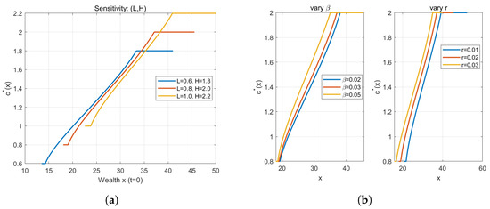
Figure 4. Sensitivity of the optimal consumption policy $c^{*}\left(x\right)$ under two-sided consumption bounds. Panel (a) compares consumption rules for different pairs of bounds $(L,H)$, illustrating how tightening the lower floor L or ceiling H compresses the feasible interior region. Panel (b) shows the effect of preference and market parameters: increasing $\beta$ or r raises near-term consumption and shortens the unconstrained range. Together, the panels demonstrate the robustness of the three-zone policy structure and the consistency between analytical comparative statics and numerical results. (a) Sensitivity to consumption bounds $(L,H)$. Lower bounds shift the curve upward at low wealth, while higher upper bounds extend the unconstrained region before saturation occurs. (b) Sensitivity to time preference $\beta$ and risk-free rate r. A higher discount rate or interest rate steepens the slope of $c^{*}\left(x\right)$, reflecting stronger impatience and wealth effects.

6. Conclusions

This paper develops a finite-horizon model of optimal consumption and investment under two-sided consumption bounds. Methodologically, our main contribution is a closed-form dual representation that remains tractable with both a lower bound L and an upper bound H on consumption. We derive normal-form integral expressions for the dual value function and its first two derivatives, establish smoothness and strict convexity of the dual cost-to-go, and obtain explicit feedback formulas:

$$X_t^{*}=-{\partial }_y\mathcal{J}(t,Y_t^{*}),{\pi }_t^{*}={\displaystyle \frac{\theta }{\sigma }}{Y}_t^{*}{\partial }_{yy}\mathcal{J}(t,Y_t^{*}),c_t^{*}={\Pi }_{[L,H]}\left(I\left(Y_t^{*}\right)\right).$$

These identities make the role of the dual process $Y_t^{*}=y^{*}{e}^{\beta t}{H}_t$ transparent and allow us to read off the qualitative shape of optimal policies directly from the sign and curvature of the dual derivatives.

Two-sided bounds transform the linear Merton rule into a three-region consumption policy (lower, interior, upper) and a curvature-driven portfolio rule. Because the shadow price $Y_t^{*}$ is inherently time-varying on a finite horizon, terminal conditions interact nontrivially with caps and floors: as $t\uparrow T$, binding probabilities and marginal values change even in a complete market. Our formulas explain when and why the optimal risky position becomes inverted-U in wealth—vanishing near both bounds—and how a stronger bequest motive offsets this effect by sustaining positive curvature ${\partial }_{yy}\mathcal{J}$ at high wealth. Thus, finite-horizon planning is first-order for both the geometry of policies and their comparative statics.

The model speaks to retirement windows and finite-lived institutions that operate under spending floors (subsistence, fixed operating costs) and ceilings (liquidity, adjustment limits, saturation). Our explicit feedback rules provide implementable diagnostics: (i) the distance of $Y_t^{*}$ from $\{u^{\prime }\left(L\right),u^{\prime }\left(H\right)\}$ gauges the likelihood of binding constraints; (ii) the sign and magnitude of ${\partial }_{yy}\mathcal{J}$ translate into risk-taking intensity; and (iii) bequest intensity (via $k_B$) shifts risky exposure at high wealth, clarifying when upper-bound saturation would otherwise suppress portfolio risk. Numerically, we quantify these mechanisms: consumption exhibits saturation at both ends, and portfolios display the predicted inverted-U in the weak-bequest case, whereas stronger bequest preferences preserve positive risky exposure for affluent agents.

In settings with liquidity regulation or spending guidelines, the analysis highlights a trade-off: raising floors protects short-run welfare but compresses risk taking at low wealth; tightening ceilings curbs overspending but may mute long-horizon risk premia unless complemented by explicit terminal objectives (bequest or funding targets). Because our characterization is closed form, one can stress-test $(L,H)$ and horizon T quickly to obtain ex ante welfare and ex post portfolio diagnostics.

The analytical feedback rules derived in this study offer direct implications for portfolio optimization and risk management in both household and institutional contexts. For individual investors, the curvature term ${\partial }_{yy}\mathcal{J}$ provides a clear diagnostic of risk-taking intensity: it decreases when consumption constraints bind, explaining why optimal portfolio exposure diminishes at both low and high wealth levels. From a household perspective, the lower bound L represents a subsistence or liquidity threshold ensuring minimal living standards, while the upper bound H captures spending inertia or psychological saturation—features consistent with observed consumption rigidity. At the institutional level, the parameters $(L,H)$ can be interpreted as policy-imposed spending floors and ceilings, allowing regulators or fund managers to assess how budget rules affect both ex ante welfare and ex post portfolio volatility. Hence, our closed-form characterization bridges theoretical optimal control with practical applications in financial planning, consumption regulation, and risk management.

Looking ahead, our framework opens several promising directions for future research. First, relaxing market completeness by allowing for unhedgeable income risk or segmented trading opportunities would make the analysis more realistic and test the robustness of the dual structure. Second, extending the model to stochastic interest rates or time-varying investment opportunities could reveal richer horizon effects. Third, incorporating behavioral features—such as habit persistence, durability, or loss aversion—would connect the two-sided bound mechanism to observed consumption rigidity and psychological thresholds. These extensions would broaden the model’s applicability while maintaining the analytical clarity of the dual-martingale approach.

We worked in a frictionless complete market with CRRA preferences and deterministic parameters. Natural extensions include incomplete markets and stochastic interest rates, richer preference specifications (e.g., durability or adjustment costs), and data-driven calibration that maps $(L,H)$ to institutional or household features. Our dual formulas provide a portable backbone for these extensions: once the state-price density is specified, the same integral machinery yields policy shapes and comparative statics.

In sum, we synthesize a mathematically explicit dual approach with economically transparent policy rules. Finite horizons and two-sided spending bounds jointly reshape consumption smoothing and portfolio choice, offering a tractable lens for retirement planning, institutional spending design, and risk management under realistic constraints.

References

- Merton, R.C. Lifetime portfolio selection under uncertainty: The continuous-time case. Rev. Econ. Stat. 1969, 51, 247–257. [Google Scholar] [CrossRef]
- Merton, R.C. Optimum consumption and portfolio rules in a continuous-time model. J. Econ. Theory 1971, 3, 373–413. [Google Scholar] [CrossRef]
- Constantinides, G.M. Habit formation: A resolution of the equity premium puzzle? J. Political Econ. 1990, 98, 519–543. [Google Scholar] [CrossRef]
- Campbell, J.Y.; Cochrane, J.H. By force of habit: A consumption-based explanation of aggregate stock market behavior. J. Political Econ. 1999, 107, 205–251. [Google Scholar] [CrossRef]
- Cox, J.C.; Huang, C.-F. Optimal consumption and portfolio policies when asset prices follow a diffusion process. J. Econ. Theory 1989, 49, 33–83. [Google Scholar] [CrossRef]
- Harrison, J.M.; Pliska, S.R. Martingales and stochastic integrals in the theory of continuous trading. Stoch. Processes Their Appl. 1981, 11, 215–260. [Google Scholar] [CrossRef]
- Harrison, J.M.; Pliska, S.R. A stochastic calculus model of continuous trading: Complete markets. Stoch. Processes Their Appl. 1983, 15, 313–316. [Google Scholar] [CrossRef]
- Karatzas, I.; Shreve, S.E. Methods of Mathematical Finance; Springer: New York, NY, USA, 1998. [Google Scholar]
- Björk, T. Arbitrage Theory in Continuous Time, 3rd ed.; Oxford University Press: Oxford, UK, 2009. [Google Scholar]
- Pham, H. Continuous-Time Stochastic Control and Optimization with Financial Applications; Springer: Berlin, Germany, 2009. [Google Scholar]
- Ma, Q.; Yi, F.; Guan, C. A consumption–investment problem with constraints on minimum and maximum consumption rates. J. Comput. Appl. Math. 2018, 338, 185–198. [Google Scholar] [CrossRef]
- El Karoui, N.; Jeanblanc-Picqué, M. Optimization of consumption with labor income. Financ. Stochastics 1998, 2, 409–440. [Google Scholar] [CrossRef]
- Cuoco, D.; He, H. Dynamic aggregation and computation of equilibria in incomplete markets. J. Econ. Dyn. Control 1994, 18, 817–851. [Google Scholar]
- Karatzas, I.; Lehoczky, J.P.; Shreve, S.E. Optimal portfolio and consumption decisions for a “small investor” on a finite horizon. SIAM J. Control Optim. 1987, 25, 1557–1586. [Google Scholar] [CrossRef]
- Kramkov, D.; Schachermayer, W. The asymptotic elasticity of utility and optimal investment in incomplete markets. Financ. Stochastics 1999, 3, 237–248. [Google Scholar] [CrossRef]
- Karatzas, I.; Žitković, G. Optimal consumption from investment and random endowment in incomplete semimartingale markets. Ann. Probab. 2003, 31, 1821–1858. [Google Scholar] [CrossRef]
- Campbell, J.Y.; Deaton, A. Why is consumption so smooth? Rev. Econ. Stud. 1989, 56, 357–374. [Google Scholar] [CrossRef]
- Carroll, C.D. Buffer-stock saving and the life cycle/permanent income hypothesis. Q. J. Econ. 1997, 112, 1–55. [Google Scholar] [CrossRef]
- Yong, J.; Zhou, X.Y. Stochastic Controls: Hamiltonian Systems and HJB Equations; Springer: New York, NY, USA, 1999. [Google Scholar]
- Øksendal, B. Stochastic Differential Equations: An Introduction with Applications, 6th ed.; Springer: Berlin, Germany, 2003. [Google Scholar]
- Grossman, S.J.; Zhou, Z. Optimal investment strategies for controlling drawdowns. J. Financ. 1993, 48, 907–937. [Google Scholar] [CrossRef]
- Jeon, J.; Oh, J. Finite horizon portfolio selection problem with a drawdown constraint on consumption. J. Math. Anal. Appl. 2022, 506, 125542. [Google Scholar] [CrossRef]
Disclaimer/Publisher’s Note: The statements, opinions and data contained in all publications are solely those of the individual author(s) and contributor(s) and not of MDPI and/or the editor(s). MDPI and/or the editor(s) disclaim responsibility for any injury to people or property resulting from any ideas, methods, instructions or products referred to in the content. |
© 2025 by the authors. Licensee MDPI, Basel, Switzerland. This article is an open access article distributed under the terms and conditions of the Creative Commons Attribution (CC BY) license (https://creativecommons.org/licenses/by/4.0/).