Robust Optimal Reinsurance and Investment Problem Under Markov Switching via Actor–Critic Reinforcement Learning

Abstract

This paper investigates a robust optimal reinsurance and investment problem for an insurance company operating in a Markov-modulated financial market. The insurer’s surplus process is modeled by a diffusion process with jumps, which is correlated with financial risky assets through a common shock structure. The economic regime switches according to a continuous-time Markov chain. To address model uncertainty concerning both diffusion and jump components, we formulate the problem within a robust optimal control framework. By applying the Girsanov theorem for semimartingales, we derive the dynamics of the wealth process under an equivalent martingale measure. We then establish the associated Hamilton–Jacobi–Bellman (HJB) equation, which constitutes a coupled system of nonlinear second-order integro-differential equations. An explicit form of the relative entropy penalty function is provided to quantify the cost of deviating from the reference model. The theoretical results furnish a foundation for numerical solutions using actor–critic reinforcement learning algorithms.

1. Introduction

The increasing integration of insurance and financial markets has created complex risk interdependence structures that pose significant challenges to traditional risk management paradigms [1,2]. This evolving landscape has motivated extensive research on optimal control problems characterized by sophisticated risk correlations. The current literature can be broadly categorized into several research streams addressing different aspects of this challenge.

One prominent research direction focuses on modeling dependence structures among insurance claims, particularly under common shock frameworks (see [3,4,5]). However, insurance companies face a dual risk exposure: underwriting risk from their insurance operations and investment risk from their asset portfolios. Crucially, these risk sources often exhibit significant positive correlation during extreme market conditions [6,7], creating amplified risk scenarios that require sophisticated management approaches. Recent work by [8] emphasizes analyzing the dual impact of common shocks on both insurance claims and financial markets, while [9] explicitly considers the correlation between risk models and risky asset prices.

The economic environment’s inherent complexity and volatility necessitate accounting for multiple market regimes (e.g., bull and bear markets) in risk modeling. The Markov regime-switching framework has emerged as a powerful tool for capturing this phenomenon, where stock returns and volatilities systematically vary with market states. Seminal work by [10] analyzed proportional reinsurance and investment strategies under regime uncertainty, establishing the foundation for this research stream. Subsequent studies by [3,11,12,13] have further investigated optimal reinsurance and investment strategies within Markov regime-switching environments, consistently demonstrating the significant impact of regime changes on asset returns and insurance claim patterns.

Model uncertainty presents another critical dimension in this research domain. Traditional investment or reinsurance models typically assume fixed or deterministically varying parameters, despite the well-documented challenges in accurately estimating these parameters, particularly expected returns of risky assets. Similar estimation uncertainties plague the surplus processes of insurance companies. The literature unequivocally shows that optimal reinsurance and investment strategies exhibit high sensitivity to model parameters, with parameter non-robustness leading to significant strategy instability. Consequently, incorporating model uncertainty into asset allocation and reinsurance processes has become imperative. The robust control approach has emerged as the primary methodology for addressing model uncertainty, operating by identifying substitute models that minimize deviation from reference models to derive robust optimal strategies under worst-case scenarios. Notable contributions in this area include [12,14,15,16,17,18], who developed comprehensive frameworks for robust optimal reinsurance and investment that accommodate model ambiguity from multiple risk sources and negative interdependence between markets.

From a modeling perspective, most existing literature concentrates on simplified financial markets comprising a single risk-free asset and one risky asset. Driven by practical requirements, several scholars have extended this basic framework. For instance, Ref. [19] incorporated defaultable risk into a jump-diffusion risk model to study mean-variance optimal reinsurance and investment problems. Meanwhile, other researchers have focused on developing more realistic market environments with multiple risky assets (see [20,21,22]), aiming to derive optimal portfolios across diverse asset classes.

The methodological approach predominantly employed in the aforementioned literature involves applying the dynamic programming principle [23] to derive corresponding Hamilton–Jacobi–Bellman (HJB) equations [24]. The standard solution methodology then utilizes the method of undetermined coefficients to solve these partial differential equations, yielding optimal reinsurance and investment strategies along with associated value functions. However, this approach suffers from significant limitations: it heavily relies on analytical intuition and educated guessing of solution forms, proves computationally intensive, and demonstrates poor performance when addressing high-dimensional HJB equations or coupled nonlinear integro-differential HJB equations.

To overcome these computational challenges, recent research has turned to reinforcement learning methods, applicable to both discrete-time and continuous-time settings. Pioneering work by [25,26,27] established rigorous theoretical foundations and convergence analyses for deep-learning-based methods in continuous-time stochastic control. More recently, [28,29] demonstrated the exceptional scalability of actor–critic algorithms in portfolio and reinsurance optimization contexts, respectively.

Despite these significant advancements, several critical research gaps remain unaddressed:

• Existing frameworks often fail to comprehensively integrate three crucial elements: risk interdependence between insurance and financial markets, Markov regime switching across economic states, and model uncertainty with decision-maker ambiguity aversion.
• Traditional solution methodologies prove inadequate for handling the resulting high-dimensional, coupled systems of nonlinear integro-differential HJB equations, creating a computational bottleneck that limits model complexity and practical applicability.

This paper makes three primary contributions to bridge these research gaps:

• We develop a comprehensive modeling framework that simultaneously incorporates Markov regime-switching effects on both the insurer’s wealth process and financial market dynamics, while explicitly capturing the interdependence between insurance claims and risky asset prices through a common shock structure.
• We formulate a robust optimal control problem that explicitly accounts for the insurer’s ambiguity aversion toward model uncertainty, enabling the derivation of conservative yet robust strategies in ambiguous environments. By establishing the corresponding HJB equations with explicit penalty functions, we significantly enhance the reliability and risk resilience of decision schemes in practical applications.
• We design an efficient numerical algorithm based on actor–critic reinforcement learning to solve the resulting system of coupled nonlinear integro-differential HJB equations. This approach effectively handles high-dimensional optimization spaces while respecting the model’s intrinsic complexity, providing a computationally feasible solution methodology for this challenging class of problems.

The remainder of this paper is organized as follows. Section 2 introduces the model setup and derives the wealth process dynamics. Section 3 formulates the robust control problem. Section 4 derives the HJB equation with explicit penalty function. Section 5 outlines the actor–critic reinforcement learning framework for solving the HJB system. Section 6 presents numerical simulations. Section 7 conducts sensitivity analyses on key parameters, and Section 8 concludes the paper.

2. Model and Assumptions

Following the framework of [6,7,24], we consider a complete probability space $(\Omega ,\mathcal{F},\mathbb{P})$ equipped with a two-dimensional Brownian motion

$${\left(W_0\left(t\right),W_1\left(t\right)\right)}_{t\ge 0}$$

whose components satisfy

$${⟨W_0,W_1⟩}_t=\rho t,\rho \in [-1,1],$$

To model economic regime shifts, we adopt the Markov regime-switching framework established in [10] and extended in [3]. Let $\left({\alpha }_t\right)t\ge 0$ be a continuous-time, finite-state Markov chain with state space $\mathcal{M}=1,\dots ,m$ and generator matrix $Q=\left(qij\right)i,j\in \mathcal{M}$. The Markov chain $\alpha t$ modulates all model parameters according to the prevailing economic regime.

The insurer’s surplus process follows the dynamics given by

$$\mathrm{d}R\left(t\right)=c(t,{\alpha }_t)\mathrm{d}t+{\sigma }_0(t,{\alpha }_t)\mathrm{d}{W}_0\left(t\right)-\mathrm{d}\left(\sum _{j=1}^{M_1(t,\alpha \left(t\right))}{X}_j\right),R\left(0\right)=R_0,$$

where $c(t,i)$ represents the premium rate in regime i, ${\sigma }_0(t,i)$ denotes the volatility coefficient of the surplus process, $\left\{W_0\left(t\right)\right\}$ is a standard Brownian motion representing small fluctuations, $\left\{M_1(t,i)\right\}$ is a Poisson process with intensity ${\lambda }_{1i}+{\lambda }_{0i}>0$, and ${\left\{X_j\right\}}_{j\ge 1}$ are independent and identically distributed claim sizes with $\mathbb{E}\left[X_j\right]={\mu }_1$ and $\mathbb{E}\left[X_j^2\right]={\beta }_1$.

The financial market consists of one risk-free asset and l risky assets. The risk-free asset price $S_0\left(t\right)$ evolves according to

$$\mathrm{d}{S}_0\left(t\right)=r_0(t,{\alpha }_t)S_0\left(t\right)\mathrm{d}t,$$

where $r_0(t,i)$ is the risk-free interest rate in regime i. For the risky assets, we extend the jump-diffusion model in [4] by incorporating regime switching and common shock dependence, unlike the conventional approach that models risky assets solely with a pure diffusion process or its local-volatility approximation. The price of the k-th risky asset $S_k\left(t\right)$ follows:

$${\displaystyle \frac{\mathrm{d}{S}_k\left(t\right)}{S_k\left(t^{-}\right)}}=r_k(t,{\alpha }_t)\mathrm{d}t+{\sigma }_k(t,{\alpha }_t)\mathrm{d}{W}_1\left(t\right)+\mathrm{d}\left(\sum _{j=1}^{M_{2k}(t,\alpha \left(t\right))}{Y}_{kj}\right),k=1,2,...,l,$$

where $r_k(t,i)$ denotes the expected return of asset k in regime i, ${\sigma }_k(t,i)$ represents the volatility coefficient, $W_1\left(t\right)$ is a standard Brownian motion, $\left\{M_{2k}(t,i)\right\}$ is a Poisson process with intensity ${\lambda }_{2k,i}+{\lambda }_{0i}$, and $\left\{Y_{kj}\right\}$ are independent and identically distributed jump sizes with $\mathbb{P}\{Y_{kj}>-1\}=1$, $\mathbb{E}\left[Y_{kj}\right]={\mu }_{2k}$, and $\mathbb{E}\left[Y_{kj}^2\right]={\beta }_{2k}$.

The dependence structure between insurance and financial markets is captured through the decomposition of the Poisson processes:

$$M_1(t,i)=N_{1i}\left(t\right)+N_{0i}\left(t\right),M_{2k}(t,i)=N_{2k}^i\left(t\right)+N_{0i}\left(t\right),$$

where $N_{1i}\left(t\right)$ represents the Poisson process for idiosyncratic insurance claims with intensity ${\lambda }_{1i}$, $N_{2k}^i\left(t\right)$ denotes the Poisson process for idiosyncratic financial jumps with intensity ${\lambda }_{2k,i}$, and $N_0^i\left(t\right)$ represents the Poisson process for common shocks with intensity ${\lambda }_{0i}$.

The wealth process $X_t^{\pi ,q}$ under the strategy $(\pi ,q)=({\pi }_1,{\pi }_2,...,{\pi }_l,q)$ satisfies the stochastic differential equation

$$\begin{array}{cc}\hfill \mathrm{d}{X}_t^{\pi ,q}=& \left[c(t,{\alpha }_t)-u(t,{\alpha }_t,q_t)+r_0(t,{\alpha }_t)\left(X_t^{\pi ,q}-\sum _{k=1}^l{\pi }_k\left(t\right)\right)+\sum _{k=1}^l{\pi }_k\left(t\right)r_k(t,{\alpha }_t)\right]\mathrm{d}t\hfill \\ \hfill & +{\sigma }_0(t,{\alpha }_t)\mathrm{d}{W}_0\left(t\right)+\left(\sum _{k=1}^l{\pi }_k\left(t\right){\sigma }_k(t,{\alpha }_t)\right)\mathrm{d}{W}_1\left(t\right)\hfill \\ \hfill & -q_t\mathrm{d}\left(\sum _{j=1}^{M_1(t,{\alpha }_t)}{X}_j\right)+\sum _{k=1}^l{\pi }_k\left(t\right)\mathrm{d}\left(\sum _{j=1}^{M_{2k}(t,{\alpha }_t)}{Y}_{kj}\right),\hfill \end{array}$$

(1)

where $u(t,{\alpha }_t,q_t)$ denotes the reinsurance premium, ${\pi }_k\left(t\right)$ represents the amount invested in asset k, and $q_t$ is the retention level satisfying $0\le q_t\le 1$. This wealth process generalizes the models in [15,16] by incorporating multiple risky assets, regime-switching, and the common shock structure.

A strategy $(\pi ,q)=({\pi }_1\left(t\right),{\pi }_2\left(t\right),...,{\pi }_l\left(t\right),q_t)$ is admissible if

• $q_t,{\pi }_1\left(t\right),{\pi }_2\left(t\right),...,{\pi }_l\left(t\right)$ are ${\mathcal{F}}_t$-predictable;
• $q_t\ge 0,{\pi }_1\left(t\right),{\pi }_2\left(t\right),...,{\pi }_l\left(t\right)\ge 0$;
• ${\displaystyle \mathbb{E}{\int }_0^T(|q_t{|}^2+\sum _{i=1}^l{\left|{\pi }_i\left(t\right)\right|}^2)\mathrm{d}t<\infty }$;
• Equation (1) has a unique strong solution.

The set of all admissible strategies is denoted by $\Pi$.

3. Robust Optimal Control Problem

Assume the insurer aims to maximize the expected utility of terminal wealth. In a traditional model, the ambiguity-neutral insurer’s objective function is

$$\underset{\pi ,q\in \Pi }{sup}{\mathbb{E}}^{\mathbb{P}}\left[U\left(R^{\pi ,q}\left(T\right)\right)\right],$$

(2)

where $\Pi$ denotes the set of admissible strategies and ${\mathbb{E}}^{\mathbb{P}}$ is the expectation under the probability measure $\mathbb{P}$.

Recent studies, however, show that investors in the market are in fact averse to ambiguity. Therefore, we incorporate ambiguity into the optimization problem and define a class of probability measures that are equivalent to $\mathbb{P}$ as alternative measures

$$\mathcal{Q}=\{\mathbb{Q}\mid \mathbb{Q}\sim \mathbb{P}\}.$$

We consider an equivalent martingale measure $\mathbb{Q}$ defined by the Radon–Nikodym derivative process

$${\Lambda }_t={\displaystyle \frac{d\mathbb{Q}}{d\mathbb{P}}}{|}_{{\mathcal{F}}_t}$$

that defines the equivalent martingale measure $\mathbb{Q}$, given by:

$$\begin{array}{cc}\hfill {\Lambda }_t=& exp\{{\int }_0^t{\theta }_{W_0}\left(s\right)d{W}_0\left(s\right)-{\displaystyle \frac{1}{2}}{\int }_0^t{\theta }_{W_0}^2\left(s\right)ds+{\int }_0^t{\theta }_{W_1}\left(s\right)d{W}_1\left(s\right)-{\displaystyle \frac{1}{2}}{\int }_0^t{\theta }_{W_1}^2\left(s\right)ds\hfill \\ \hfill & +\sum _{i=1}^m{\int }_0^t{\int }_0^{\infty }ln(1+{\gamma }_1(s,z,i)){\tilde{N}}_{1i}(ds,dz)\hfill \\ \hfill & +{\int }_0^t{\int }_0^{\infty }[ln(1+{\gamma }_1(s,z,i))-{\gamma }_1(s,z,i)]{\lambda }_{1i}{F}_1\left(dz\right)ds\hfill \\ \hfill & +\sum _{i=1}^m\sum _{k=1}^l{\int }_0^t{\int }_{-\infty }^{\infty }ln(1+{\gamma }_{2k}(s,y,i)){\tilde{N}}_{2k,i}(ds,dy)\hfill \\ \hfill & +{\int }_0^t{\int }_{-\infty }^{\infty }[ln(1+{\gamma }_{2k}(s,y,i))-{\gamma }_{2k}(s,y,i)]{\lambda }_{2k,i}{F}_{2k}\left(dy\right)ds\},\hfill \end{array}$$

(3)

where ${\theta }_{W_0}\left(t\right)$ and ${\theta }_{W_1}\left(t\right)$ are the market prices of diffusion risk, ${\gamma }_1(t,z,i)$ is the market price of insurance jump risk, ${\gamma }_{2k}(t,y,i)$ is the market price of financial jump risk for asset k, ${\tilde{N}}_{1i}$ and ${\tilde{N}}_{2k,i}$ are the compensated Poisson random measures under $\mathbb{P}$, ${\lambda }_{1i}$ and ${\lambda }_{2k,i}$ are the jump intensities under $\mathbb{P}$, and $F_1$ and $F_{2k}$ are the jump size distributions under $\mathbb{P}$.

This process ${\Lambda }_t$ serves as the likelihood ratio that transforms the original probability measure $\mathbb{P}$ to the equivalent martingale measure $\mathbb{Q}$, adjusting for both diffusion and jump risks in the market.

The measure transformation from $\mathbb{P}$ to $\mathbb{Q}$ involves three main components: Brownian motions, Poisson processes, and Markov chain transitions. By Girsanov’s theorem, the $\mathbb{Q}$-Brownian motions relate to the $\mathbb{P}$-Brownian motions through the transformations:

$$\mathrm{d}{\tilde{W}}_0\left(t\right)=\mathrm{d}{W}_0\left(t\right)-{\theta }_{W_0}\left(t\right)\mathrm{d}t,$$

$$\mathrm{d}{\tilde{W}}_1\left(t\right)=\mathrm{d}{W}_1\left(t\right)-{\theta }_{W_1}\left(t\right)\mathrm{d}t.$$

whose components satisfy

$${⟨{\tilde{W}}_0,{\tilde{W}}_1⟩}_t=\rho t,\rho \in [-1,1].$$

For the jump processes, the intensity and jump size distribution change under $\mathbb{Q}$. Denote ${\tilde{N}}_1\left(t\right)$ as the compensated insurance jump process under $\mathbb{Q}$:

$$\mathrm{d}{\tilde{N}}_1\left(t\right)=\mathrm{d}\left(\sum _{j=1}^{M_1(t,{\alpha }_t)}{X}_j\right)-{\lambda }_{1,{\alpha }_t}\left({\mu }_X+{\int }_0^{\infty }z{\gamma }_1(t,z,{\alpha }_t)F_1\left(\mathrm{d}z\right)\right)\mathrm{d}t.$$

where ${\mu }_X={\int }_0^{\infty }z{F}_1\left(\mathrm{d}z\right)$ is the mean insurance claim size under $\mathbb{P}$. Denote ${\tilde{N}}_{2k}\left(t\right)$ as the compensated financial jump process for asset k under $\mathbb{Q}$:

$$\mathrm{d}{\tilde{N}}_{2k}\left(t\right)=\mathrm{d}\left(\sum _{j=1}^{M_{2k}(t,{\alpha }_t)}{Y}_{kj}\right)-{\lambda }_{2k,{\alpha }_t}\left({\mu }_{Y_k}+{\int }_{-\infty }^{\infty }y{\gamma }_{2k}(t,y,{\alpha }_t)F_{2k}\left(\mathrm{d}y\right)\right)\mathrm{d}t.$$

where ${\mu }_{Y_k}={\int }_{-\infty }^{\infty }y{F}_{2k}\left(\mathrm{d}y\right)$ is the mean jump size for asset k under $\mathbb{P}$.

Theorem 1

(Wealth Process under $\mathbb{Q}$). The wealth process $X_t^{\pi ,q}$ under the equivalent martingale measure $\mathbb{Q}$ satisfies the following stochastic differential equation (SDE):

$$\begin{array}{cc}\hfill \mathrm{d}{X}_t^{\pi ,q}=& \left[c(t,{\alpha }_t)-u(t,{\alpha }_t,q_t)+r_0(t,{\alpha }_t)\left(X_t^{\pi ,q}-\sum _{k=1}^l{\pi }_k\left(t\right)\right)+\sum _{k=1}^l{\pi }_k\left(t\right)r_k(t,{\alpha }_t)\right.\hfill \\ \hfill & +{\sigma }_0(t,{\alpha }_t){\theta }_{W_0}\left(t\right)+\left(\sum _{k=1}^l{\pi }_k\left(t\right){\sigma }_k(t,{\alpha }_t)\right){\theta }_{W_1}\left(t\right)\hfill \\ \hfill & -q_t{\lambda }_{1,{\alpha }_t}\left({\mu }_X+{\int }_0^{\infty }z{\gamma }_1(t,z,{\alpha }_t)F_1\left(\mathrm{d}z\right)\right)\hfill \\ \hfill & \left.+\sum _{k=1}^l{\pi }_k\left(t\right){\lambda }_{2k,{\alpha }_t}\left({\mu }_{Y_k}+{\int }_{-\infty }^{\infty }y{\gamma }_{2k}(t,y,{\alpha }_t)F_{2k}\left(\mathrm{d}y\right)\right)\right]\mathrm{d}t\hfill \\ \hfill & +{\sigma }_0(t,{\alpha }_t)\mathrm{d}{\tilde{W}}_0\left(t\right)+\left(\sum _{k=1}^l{\pi }_k\left(t\right){\sigma }_k(t,{\alpha }_t)\right)\mathrm{d}{\tilde{W}}_1\left(t\right)\hfill \\ \hfill & -q_t\mathrm{d}{\tilde{N}}_1\left(t\right)+\sum _{k=1}^l{\pi }_k\left(t\right)\mathrm{d}{\tilde{N}}_{2k}\left(t\right),\hfill \end{array}$$

(4)

Proof. 

We begin with the wealth process under the physical measure $\mathbb{P}$:

$$\begin{array}{cc}\hfill \mathrm{d}{X}_t^{\pi ,q}=& \left[c(t,{\alpha }_t)-u(t,{\alpha }_t,q_t)+r_0(t,{\alpha }_t)\left(X_t^{\pi ,q}-\sum _{k=1}^l{\pi }_k\left(t\right)\right)+\sum _{k=1}^l{\pi }_k\left(t\right)r_k(t,{\alpha }_t)\right]\mathrm{d}t\hfill \\ \hfill & +{\sigma }_0(t,{\alpha }_t)\mathrm{d}{W}_0\left(t\right)+\left(\sum _{k=1}^l{\pi }_k\left(t\right){\sigma }_k(t,{\alpha }_t)\right)\mathrm{d}{W}_1\left(t\right)\hfill \\ \hfill & -q_t\mathrm{d}\left(\sum _{j=1}^{M_1(t,{\alpha }_t)}{X}_j\right)+\sum _{k=1}^l{\pi }_k\left(t\right)\mathrm{d}\left(\sum _{j=1}^{M_{2k}(t,{\alpha }_t)}{Y}_{kj}\right).\hfill \end{array}$$

Applying Girsanov’s theorem for semimartingales, we transform the Brownian motions:

$$\begin{array}{cc}\hfill d{\tilde{W}}_0\left(t\right)& =d{W}_0\left(t\right)-{\theta }_{W_0}\left(t\right)dt,\hfill \\ \hfill d{\tilde{W}}_1\left(t\right)& =d{W}_1\left(t\right)-{\theta }_{W_1}\left(t\right)dt.\hfill \end{array}$$

For the jump components, under the equivalent measure $\mathbb{Q}$, the compensated jump processes become:

$$\begin{array}{cc}\hfill d{\tilde{N}}_1\left(t\right)& =d\left(\sum _{j=1}^{M_1(t,{\alpha }_t)}{X}_j\right)-{\lambda }_{1,{\alpha }_t}\left({\mu }_X+{\int }_0^{\infty }z{\gamma }_1(t,z,{\alpha }_t)F_1\left(dz\right)\right)dt,\hfill \\ \hfill d{\tilde{N}}_{2k}\left(t\right)& =d\left(\sum _{j=1}^{M_{2k}(t,{\alpha }_t)}{Y}_{kj}\right)-{\lambda }_{2k,{\alpha }_t}\left({\mu }_{Y_k}+{\int }_{-\infty }^{\infty }y{\gamma }_{2k}(t,y,{\alpha }_t)F_{2k}\left(dy\right)\right)dt.\hfill \end{array}$$

Substituting these transformations into the original wealth process and collecting terms, we obtain the $\mathbb{Q}$-dynamics:

$$\begin{array}{cc}\hfill d{X}_t^{\pi ,q}=& \left[c(t,{\alpha }_t)-u(t,{\alpha }_t,q_t)+r_0(t,{\alpha }_t)\left(X_t^{\pi ,q}-\sum _{k=1}^l{\pi }_k\left(t\right)\right)+\sum _{k=1}^l{\pi }_k\left(t\right)r_k(t,{\alpha }_t)\right.\hfill \\ \hfill & +{\sigma }_0(t,{\alpha }_t){\theta }_{W_0}\left(t\right)+\left(\sum _{k=1}^l{\pi }_k\left(t\right){\sigma }_k(t,{\alpha }_t)\right){\theta }_{W_1}\left(t\right)\hfill \\ \hfill & -q_t{\lambda }_{1,{\alpha }_t}\left({\mu }_X+{\int }_0^{\infty }z{\gamma }_1(t,z,{\alpha }_t)F_1\left(dz\right)\right)\hfill \\ \hfill & +\left.\sum _{k=1}^l{\pi }_k\left(t\right){\lambda }_{2k,{\alpha }_t}\left({\mu }_{Y_k}+{\int }_{-\infty }^{\infty }y{\gamma }_{2k}(t,y,{\alpha }_t)F_{2k}\left(dy\right)\right)\right]dt\hfill \\ \hfill & +{\sigma }_0(t,{\alpha }_t)d{\tilde{W}}_0\left(t\right)+\left(\sum _{k=1}^l{\pi }_k\left(t\right){\sigma }_k(t,{\alpha }_t)\right)d{\tilde{W}}_1\left(t\right)\hfill \\ \hfill & -q_{t}d{\tilde{N}}_1\left(t\right)+\sum _{k=1}^l{\pi }_k\left(t\right)d{\tilde{N}}_{2k}\left(t\right).\hfill \end{array}$$

This completes the proof of Theorem 1. □

Following Reference [30], to rectify problem (2), we formulate a robust optimal problem

$$V(t,x,i,S)=\underset{\pi ,q}{sup}\underset{\theta ,\gamma }{inf}{\mathbb{E}}_{t,x,i}^{\mathbb{Q}}\left[U\left(X_T^{\pi }\right)+{\int }_t^T\psi (s,X_s^{\pi },{\theta }_s,{\gamma }_s)\mathrm{d}s\right],$$

(5)

where ${\mathbb{E}}^Q[·]$ denotes the expectation under the alternative measure Q, and $\psi \left(s,R^{\ast }\left(s\right),\pi \left(s\right)\right)$ is the discounted relative entropy that penalizes the discrepancy between the reference model and the alternative model.

4. Hamilton–Jacobi–Bellman Equation

Before establishing the main theorems, we first present the technical conditions that ensure the existence and uniqueness of solutions to the robust HJB equation.

Assume the following conditions hold:

(i)

Coefficient Regularity Conditions: There exists a constant $K>0$ such that for all $t\in [0,T]$, $x,y\in \mathbb{R}$, $i\in \mathcal{M}$:

$$\begin{array}{cc}\hfill & |c(t,i,x)-c(t,i,y)|+|{\sigma }_0(t,i,x)-{\sigma }_0(t,i,y)|\le K|x-y|\hfill \\ \hfill & \sum _{k=1}^l\left(|r_k(t,i,x)-r_k(t,i,y)|+|{\sigma }_k(t,i,x)-{\sigma }_k(t,i,y)|\right)\le K|x-y|\hfill \\ \hfill & \left|c(t,i,x)\right|+|{\sigma }_0(t,i,x)|+\sum _{k=1}^l\left(|r_k(t,i,x)|+|{\sigma }_k(t,i,x)|\right)\le K(1+|x\left|\right)\hfill \end{array}$$

(ii)

Uniform Ellipticity Condition: There exists $\epsilon >0$ such that for any admissible strategy $(\pi ,q)\in \Pi$:

$${\sigma }_0^2(t,i)+{\left(\sum _{k=1}^l{\pi }_k{\sigma }_k(t,i)\right)}^2\ge \epsilon ,\forall t\in [0,T],i\in \mathcal{M}$$

(iii)

Jump Process Regularity:

$$\begin{array}{cc}\hfill & {\lambda }_{1i},{\lambda }_{2k,i},{\lambda }_{0i}\in [0,{\Lambda }_{max}],{\Lambda }_{max}<\infty \hfill \\ \hfill & {\int }_0^{\infty }{z}^2{F}_1\left(dz\right)+\underset{1\le k\le l}{max}{\int }_{-\infty }^{\infty }{y}^2{F}_{2k}\left(dy\right)<\infty \hfill \\ \hfill & \mathbb{E}\left[\right|X_j{|}^p]<\infty ,\mathbb{E}[|Y_{kj}{|}^p]<\infty ,\mathrm{for}\mathrm{some}p>2\hfill \end{array}$$

(iv)

Utility Function Conditions: The terminal utility function $U\left(x\right)$ satisfies:

$$\begin{array}{cc}\hfill & U\in C^2\left(\mathbb{R}\right),U^{\prime }\left(x\right)>0,U^{″}\left(x\right)<0\hfill \\ \hfill & \left|U\left(x\right)\right|\le C_1{(1+|x|}^p),|U^{\prime }\left(x\right)|\le C_2{(1+|x|}^{p-1})\hfill \\ \hfill & \underset{x\to 0}{lim}{U}^{\prime }\left(x\right)=\infty ,\underset{x\to \infty }{lim}{U}^{\prime }\left(x\right)=0\hfill \end{array}$$

(v)

Penalty Function Convexity: The relative entropy penalty function $\psi (t,x,\theta ,\gamma ,i)$ is strictly convex in $(\theta ,\gamma )$, and:

$${\varphi }_{W_0},{\varphi }_{W_1},{\varphi }_{1i},{\varphi }_{2k,i}\ge {\varphi }_{min}>0$$

(vi)

Measure Transformation Admissibility:

$$\begin{array}{cc}\hfill & \mathbb{E}\left[exp\left({\displaystyle \frac{1}{2}}{\int }_0^T({\theta }_{W_0}^2\left(s\right)+{\theta }_{W_1}^2\left(s\right))ds\right)\right]<\infty \hfill \\ \hfill & {\int }_0^T{\int }_{\mathbb{R}}{\left|{\gamma }_1(s,z,i)\right|}^2{F}_1\left(dz\right)ds<\infty \mathbb{P}\text{-}\mathrm{a}.\mathrm{s}.\hfill \\ \hfill & {\int }_0^T{\int }_{\mathbb{R}}{\left|{\gamma }_{2k}(s,y,i)\right|}^2{F}_{2k}\left(dy\right)ds<\infty \mathbb{P}\text{-}\mathrm{a}.\mathrm{s}.\hfill \end{array}$$

Under the above conditions, the value function $V(t,x,i)$ satisfies:

• Polynomial growth: $\left|V(t,x,i)\right|\le C(1+|x{|}^p)$
• Lipschitz continuity: $\left|V\right(t,x,i)-V(t,y,i\left)\right|\le L|x-y|$
• Semiconcavity: There exists $C>0$ such that $V(t,x,i)-{C\left|x\right|}^2$ is concave.

Theorem 2

(Robust HJB Equation). The value function $V(t,x,i)$ satisfies the following robust HJB equation:

$$\begin{array}{cc}\hfill 0=& {\displaystyle \frac{\partial V}{\partial t}}(t,x,i)+\underset{q,\pi }{sup}\underset{\theta ,\gamma }{inf}\{{\mathcal{A}}^{\pi ,q,\theta ,\gamma }V(t,x,i)+\psi (t,x,\theta ,\gamma ,i)\}\hfill \\ \hfill & \mathit{subject}\mathit{to}\mathit{the}\mathit{terminal}\mathit{condition}:V(T,x,i)=U\left(x\right),\hfill \end{array}$$

(6)

where the infinitesimal generator ${\mathcal{A}}^{\pi ,q,\theta ,\gamma }$ takes the form:

$$\begin{array}{cc}\hfill {\mathcal{A}}^{\pi ,q,\theta ,\gamma }V=& [c(t,i)-u(t,i,q)+r_0(t,i)x\hfill \\ \hfill & +\sum _{k=1}^l{\pi }_k\left(r_k(t,i)-r_0(t,i)\right)\hfill \\ \hfill & +{\sigma }_0(t,i){\theta }_{W_0}\left(t\right)+\left(\sum _{k=1}^l{\pi }_k{\sigma }_k(t,i)\right){\theta }_{W_1}\left(t\right)\hfill \\ \hfill & -q{\lambda }_{1i}^{\mathbb{Q}}{\mu }_{1i}^{\mathbb{Q}}+\sum _{k=1}^l{\pi }_k{\lambda }_{2k,i}^{\mathbb{Q}}{\mu }_{2k,i}^{\mathbb{Q}}]{\displaystyle \frac{\partial V}{\partial x}}\hfill \\ \hfill & +{\displaystyle \frac{1}{2}}\left[{\sigma }_0^2(t,i)+{\left(\sum _{k=1}^l{\pi }_k{\sigma }_k(t,i)\right)}^2\right]{\displaystyle \frac{{\partial }^{2}V}{\partial x^2}}\hfill \\ \hfill & +{\lambda }_{1i}^{\mathbb{Q}}{\int }_0^{\infty }\left[V(t,x-qz,i)-V(t,x,i)\right]F_{1i}^{\mathbb{Q}}\left(\mathrm{d}z\right)\hfill \\ \hfill & +\sum _{k=1}^l{\lambda }_{2k,i}^{\mathbb{Q}}{\int }_{-\infty }^{\infty }\left[V(t,x+{\pi }_{k}y,i)-V(t,x,i)\right]F_{2k,i}^{\mathbb{Q}}\left(\mathrm{d}y\right)\hfill \\ \hfill & +\sum _{j\in \mathcal{M}}{q}_{ij}\left[V(t,x,j)-V(t,x,i)\right]\hfill \end{array}$$

(7)

The penalty function ψ, which measures the cost of model deviation, is given by:

$$\begin{array}{cc}\hfill \psi (t,x,\theta ,\gamma ,i)& ={\displaystyle \frac{1}{2{\varphi }_{W_0}}}{\theta }_{W_0}^2\left(t\right)+{\displaystyle \frac{1}{2{\varphi }_{W_1}}}{\theta }_{W_1}^2\left(t\right)\hfill \\ \hfill +& {\displaystyle \frac{1}{{\varphi }_{1i}}}{\int }_0^{\infty }\left((1+{\gamma }_1(t,z,i))ln(1+{\gamma }_1(t,z,i))-{\gamma }_1(t,z,i)\right){\lambda }_{1i}{F}_1\left(\mathrm{d}z\right)\hfill \\ \hfill +& \sum _{k=1}^l{\displaystyle \frac{1}{{\varphi }_{2k,i}}}{\int }_{-\infty }^{\infty }\left((1+{\gamma }_{2k}(t,y,i))ln(1+{\gamma }_{2k}(t,y,i))-{\gamma }_{2k}(t,y,i)\right){\lambda }_{2k,i}{F}_{2k}\left(\mathrm{d}y\right)\hfill \end{array}$$

(8)

where

• ${\lambda }_{1i}^{\mathbb{Q}}={\lambda }_{1i}{\mathbb{E}}^{\mathbb{P}}[1+{\gamma }_1\left(z\right)]$: Insurance claim intensity under $\mathbb{Q}$ measure
• ${\mu }_{1i}^{\mathbb{Q}}={\displaystyle \frac{{\mathbb{E}}^{\mathbb{P}}\left[z(1+{\gamma }_1\left(z\right))\right]}{{\mathbb{E}}^{\mathbb{P}}[1+{\gamma }_1\left(z\right)]}}$: Average claim size under $\mathbb{Q}$ measure
• ${\lambda }_{2k,i}^{\mathbb{Q}}={\lambda }_{2k,i}{\mathbb{E}}^{\mathbb{P}}[1+{\gamma }_{2k}\left(y\right)]$: Jump intensity of asset k under $\mathbb{Q}$ measure
• ${\mu }_{2k,i}^{\mathbb{Q}}={\displaystyle \frac{{\mathbb{E}}^{\mathbb{P}}\left[y(1+{\gamma }_{2k}\left(y\right))\right]}{{\mathbb{E}}^{\mathbb{P}}[1+{\gamma }_{2k}\left(y\right)]}}$: Average jump size of asset k under $\mathbb{Q}$ measure
• ${\varphi }_{W_0}$: Ambiguity-aversion parameter for the diffusion risk of the insurer’s own surplus process
• ${\varphi }_{W_1}$: Ambiguity-aversion parameter for the diffusion risk of the financial market
• ${\varphi }_{1i}$: Ambiguity-aversion parameter for the jump risk of insurance claims
• ${\varphi }_{2k,i}$: Ambiguity-aversion parameter for the jump risk of the k-th risky asset

Proof. 

We consider the robust optimization problem:

$$V(t,x,i)=\underset{\pi ,q}{sup}\underset{\theta ,\gamma }{inf}{\mathbb{E}}_{t,x,i}^{\mathbb{Q}}\left[U\left(X_T\right)+{\int }_t^T\psi (s,X_s,{\theta }_s,{\gamma }_s,i)ds\right].$$

Applying the dynamic programming principle under model uncertainty, the value function satisfies:

$$0={\displaystyle \frac{\partial V}{\partial t}}(t,x,i)+\underset{\pi ,q}{sup}\underset{\theta ,\gamma }{inf}\left\{A^{\pi ,q,\theta ,\gamma }V(t,x,i)+\psi (t,x,\theta ,\gamma ,i)\right\},$$

with terminal condition $V(T,x,i)=U\left(x\right)$.

The infinitesimal generator $A^{\pi ,q,\theta ,\gamma }$ is derived by applying Itô’s formula for semimartingales to $V(t,X_t,{\alpha }_t)$. For a fixed regime i, we have:

$$\begin{array}{cc}\hfill A^{\pi ,q,\theta ,\gamma }V=& \left[c(t,i)-u(t,i,q)+r_0(t,i)x+\sum _{k=1}^l{\pi }_k(r_k(t,i)-r_0(t,i))\right.\hfill \\ \hfill & +{\sigma }_0(t,i){\theta }_{W_0}\left(t\right)+\left(\sum _{k=1}^l{\pi }_k{\sigma }_k(t,i)\right){\theta }_{W_1}\left(t\right)\hfill \\ \hfill & -q{\lambda }_{1i}^{\mathbb{Q}}{\mu }_{1i}^{\mathbb{Q}}+\left.\sum _{k=1}^l{\pi }_k{\lambda }_{2k,i}^{\mathbb{Q}}{\mu }_{2k,i}^{\mathbb{Q}}\right]{\displaystyle \frac{\partial V}{\partial x}}\hfill \\ \hfill & +{\displaystyle \frac{1}{2}}\left[{\sigma }_0^2(t,i)+{\left(\sum _{k=1}^l{\pi }_k{\sigma }_k(t,i)\right)}^2\right]{\displaystyle \frac{{\partial }^{2}V}{\partial x^2}}\hfill \\ \hfill & +{\lambda }_{1i}^{\mathbb{Q}}{\int }_0^{\infty }[V(t,x-qz,i)-V(t,x,i)]F_{1i}^{\mathbb{Q}}\left(dz\right)\hfill \\ \hfill & +\sum _{k=1}^l{\lambda }_{2k,i}^{\mathbb{Q}}{\int }_{-\infty }^{\infty }[V(t,x+{\pi }_{k}y,i)-V(t,x,i)]F_{2k,i}^{\mathbb{Q}}\left(dy\right)\hfill \\ \hfill & +\sum _{j\in \mathcal{M}}{q}_{ij}[V(t,x,j)-V(t,x,i)],\hfill \end{array}$$

where the $\mathbb{Q}$-measure intensities and jump size distributions are given by:

$$\begin{array}{cc}\hfill {\lambda }_{1i}^{\mathbb{Q}}& ={\lambda }_{1i}{\mathbb{E}}^{\mathbb{P}}[1+{\gamma }_1\left(z\right)],\hfill \\ \hfill {\mu }_{1i}^{\mathbb{Q}}& ={\displaystyle \frac{{\mathbb{E}}^{\mathbb{P}}\left[z(1+{\gamma }_1\left(z\right))\right]}{{\mathbb{E}}^{\mathbb{P}}[1+{\gamma }_1\left(z\right)]}},\hfill \\ \hfill {\lambda }_{2k,i}^{\mathbb{Q}}& ={\lambda }_{2k,i}{\mathbb{E}}^{\mathbb{P}}[1+{\gamma }_{2k}\left(y\right)],\hfill \\ \hfill {\mu }_{2k,i}^{\mathbb{Q}}& ={\displaystyle \frac{{\mathbb{E}}^{\mathbb{P}}\left[y(1+{\gamma }_{2k}\left(y\right))\right]}{{\mathbb{E}}^{\mathbb{P}}[1+{\gamma }_{2k}\left(y\right)]}}.\hfill \end{array}$$

The penalty function $\psi$ represents the relative entropy rate between $\mathbb{Q}$ and $\mathbb{P}$:

$$\begin{array}{cc}\hfill \psi (t,x,\theta ,\gamma ,i)=& {\displaystyle \frac{1}{2{\varphi }_{W_0}}}{\theta }_{W_0}^2\left(t\right)+{\displaystyle \frac{1}{2{\varphi }_{W_1}}}{\theta }_{W_1}^2\left(t\right)\hfill \\ \hfill & +{\displaystyle \frac{1}{{\varphi }_{1i}}}{\int }_0^{\infty }((1+{\gamma }_1(t,z,i))ln(1+{\gamma }_1(t,z,i))-{\gamma }_1(t,z,i)){\lambda }_{1i}{F}_1\left(dz\right)\hfill \\ \hfill & +\sum _{k=1}^l{\displaystyle \frac{1}{{\varphi }_{2k,i}}}{\int }_{-\infty }^{\infty }((1+{\gamma }_{2k}(t,y,i))ln(1+{\gamma }_{2k}(t,y,i))-{\gamma }_{2k}(t,y,i)){\lambda }_{2k,i}{F}_{2k}\left(dy\right).\hfill \end{array}$$

This penalty function quantifies the cost of deviating from the reference model $\mathbb{P}$, with the ambiguity-aversion parameters $\varphi$ controlling the penalty strength for each risk source.

The coupled system of nonlinear integro-differential equations arises from the regime-switching nature of the problem, where the value function in each regime depends on the value functions in all other regimes through the Markov chain generator Q.

This completes the proof of Theorem 2. □

The generator ${\mathcal{A}}^{\pi ,q,\theta ,\gamma }$ is obtained by applying Ito’s formula for semimartingales to the value function $V(t,X_t^{\pi },{\alpha }_t,S_t)$, incorporating drift terms from diffusion components, second-order terms from quadratic variation, integral terms from jump components, and transition terms from the Markov chain. The penalty function $\psi$ represents the relative entropy rate between $\mathbb{Q}$ and $\mathbb{P}$, penalizing large deviations from the reference model, with its specific form derived by computing the instantaneous relative entropy for each risk source.

5. Actor–Critic Reinforcement Learning Framework

The Hamilton–Jacobi–Bellman (HJB) equation arising from our financial optimization problem constitutes a high-dimensional, coupled nonlinear integro-differential equation that presents significant computational challenges. Traditional analytical and numerical methods, such as finite difference schemes or finite element methods, face severe limitations due to the curse of dimensionality and the non-local nature of the integral terms originating from the Lévy processes. The coupling between different state variables and the nonlinearities introduced by the utility maximization objective further complicate direct numerical solutions, motivating our adoption of an actor–critic reinforcement learning framework as a computationally feasible alternative.

This actor–critic approach is particularly well-suited for solving the HJB equation in our financial optimization problem because the continuous state and action spaces inherent in portfolio optimization naturally align with the function approximation capabilities of deep neural networks. The framework elegantly separates policy evaluation (critic) from policy improvement (actor), providing stable learning dynamics compared to pure policy gradient methods, while temporal difference learning efficiently leverages the Markovian structure of the problem, enabling online learning without requiring complete episode rollouts.

Our implementation utilizes Python 3.8+ with key scientific computing libraries: PyTorch 1.9+ for automatic differentiation and neural network construction, NumPy for numerical computations, and SciPy for additional mathematical routines. The Monte Carlo simulations leverage vectorized operations for efficient sampling of Lévy processes.

We now embed the HJB equation within this actor–critic reinforcement learning framework. The state is defined as $s_t=(t,x_t,{\alpha }_t)$, while actions are represented by $a_t=(q_t,{\pi }_{1,t},\dots ,{\pi }_{l,t})$. The value function approximation is given by $V_{\theta }\left(s_t\right)\approx V(t,x_t,{\alpha }_t)$, and the policy is denoted by ${\pi }_{\varphi }\left(a_t\right|s_t)$.

The critic network employs a single-hidden-layer architecture with parameters $\theta =(W_2,b_1,w_2,b_2)\in {\mathbb{R}}^p$, expressed as

$$V_{\theta }\left(s\right)=-w_2^{\top }tanh(W_{2}s+b_1)-b_2,$$

where the input $s={[t,x,i]}^{\top }\in {\mathbb{R}}^3$ and the hidden layer contains H neurons. The actor network generates each action dimension through independent Gaussian heads:

$$a^{\left(j\right)}\sim \mathcal{N}\left({\mu }_j(s;{\varphi }_j),{\sigma }_j^2(s;{\varphi }_j)\right),j=0,\dots ,l,$$

where $a^{\left(0\right)}=q_t$ and $a^{\left(j\right)}={\pi }_{j,t}$ for $j\ge 1$.

The instantaneous reward collected during $[t,t+\Delta t]$ is defined as $r_t=-\psi (t,s_t,a_t)$, with $\psi$ given by the explicit penalty function and evaluated through Monte Carlo sampling of the Lévy integrals. The temporal difference error is computed as

$${\delta }_t=r_t+\gamma V_{\theta }\left(s_{t+1}\right)-V_{\theta }\left(s_t\right),$$

where $\gamma =e^{-m{r}_0\Delta t}$ represents the discount factor.

For the critic network, the gradient of the loss function is given by

$${\nabla }_{\theta }{\mathcal{L}}_{\mathrm{critic}}={\delta }_t{\nabla }_{\theta }{V}_{\theta }\left(s_t\right),$$

with detailed gradients provided for each network parameter. For the actor network, the gradient for each Gaussian head is computed as

$${\nabla }_{{\varphi }_j}log{\pi }_j\left(a^{\left(j\right)}\right|s)={\displaystyle \frac{a^{\left(j\right)}-{\mu }_j}{{\sigma }_j^2}}{\nabla }_{{\varphi }_j}{\mu }_j+\left({\displaystyle \frac{{(a^{\left(j\right)}-{\mu }_j)}^2}{{\sigma }_j^2}}-1\right){\displaystyle \frac{{\nabla }_{{\varphi }_j}{\sigma }_j}{{\sigma }_j}},$$

with an additional entropy bonus gradient ${\nabla }_{{\varphi }_j}\mathcal{H}\left({\pi }_j\right)={\displaystyle \frac{1}{{\sigma }_j}}{\nabla }_{{\varphi }_j}{\sigma }_j$.

The actor parameters are updated using stochastic gradient ascent:

$${\varphi }_j\leftarrow {\varphi }_j+{\alpha }_a[{\delta }_t{\nabla }_{{\varphi }_j}log{\pi }_j+\beta {\nabla }_{{\varphi }_j}\mathcal{H}\left({\pi }_j\right)].$$

The training algorithm proceeds through the following steps: observe the current state $s_t=(t,x_t,{\alpha }_t)$ and sample an action $a_t\sim {\pi }_{\varphi }(·|s_t)$; compute the reward $r_t$ via Monte Carlo quadrature; simulate the next state $s_{t+1}$ under the $\mathbb{Q}$-dynamics; compute the temporal difference error ${\delta }_t$; update the critic parameters

$$\theta \leftarrow \theta -{\alpha }_c{\delta }_t{\nabla }_{\theta }{V}_{\theta }\left(s_t\right);$$

and update each actor parameter ${\varphi }_j$ using the corresponding gradient. The implementation employs PyTorch’s automatic differentiation for gradient computations and Adam optimizers for parameter updates, while the Monte Carlo sampling of Lévy integrals utilizes efficient vectorized operations with NumPy to ensure computational efficiency.

6. Numerical Simulation

This section presents numerical simulations based on our theoretical framework. The planning horizon is set to $T=10$ years with a time step of $\Delta t=0.01$ year. $R_0=10.$ We consider a regime-switching Markov chain with state space $\mathcal{M}=\{1,2\}$ and generator matrix

$$Q=\left(\begin{array}{cc}-0.5& 0.5\\ 0.3& -0.3\end{array}\right),$$

where state 1 represents a bull market and state 2 represents a bear market.

Table 1 lists the risk model related parameters for the bull-market state (regime 1) and the bear-market state (regime 2).

Table 1. Regime-dependent coefficients.

Parameter	Bull Market ($\mathit{i}=1$)	Bear Market ($\mathit{i}=2$)
Risk-free rate $r_0(t,i)$	0.03	0.01
Premium rate $c(t,i)$	1.5	1.2
Claim intensity ${\lambda }_{1i}$	0.8	1.2
Risky asset jump intensity ${\lambda }_{2k,i}$	0.6	0.9
Common-shock intensity ${\lambda }_{0i}$	0.10	0.30
Safety loading $\gamma \left(i\right)$	1.2	1.5

Table 2 summarises the regime-dependent expected returns and volatilities for the two risky assets.

Table 2. Risky asset parameters.

Asset k	Expected Return ${\mathit{r}}_{\mathit{k}}(\mathit{t},\mathit{i})$		Volatility ${\mathit{\sigma }}_{\mathit{k}}(\mathit{t},\mathit{i})$
	Bull Market	Bear Market	Bull Market	Bear Market
1	0.08	0.02	0.20	0.30
2	0.07	0.015	0.25	0.35

Insurance claim sizes are assumed to follow an exponential distribution with mean ${\mu }_1=1$ and variance ${\beta }_1=2$, while the jump sizes of both risky assets are modelled as log-normal random variables with log-mean ${\mu }_Y=0.05$ and log-variance ${\sigma }_Y^2=0.01$. The instantaneous correlation between the two Brownian motions driving the surplus and asset returns is set to $\rho =0.2$.

To deeply analyze the value of the robust control framework, we designed a comparative experiment: in the benchmark robust model, we assign an ambiguity-aversion coefficient ${\varphi }_{W_0}=2.0$ to the diffusion risk of the insurer’s surplus process, and ${\varphi }_{W_1}=2.0$ to the diffusion risk of the financial market. For jump risks, we use ${\varphi }_{1i}=0.5$ for insurance claims and ${\varphi }_{2k,i}=1.0$ for each risky asset $k=1,2$.

The critic network is trained with learning rate ${\eta }_0=1\times {10}^{-3}$, while the reinsurance–actor and investment–actor networks both use learning rates ${\eta }_q={\eta }_{\pi }=5\times {10}^{-4}$. An entropy regularisation coefficient ${\lambda }_q={\lambda }_{\pi }=1\times {10}^{-2}$ is applied to encourage exploration. The critic contains a single hidden layer of 64 neurons, and each Gaussian policy head in the actor contains 32 neurons. Monte Carlo integration is performed with 2000 samples per time step.

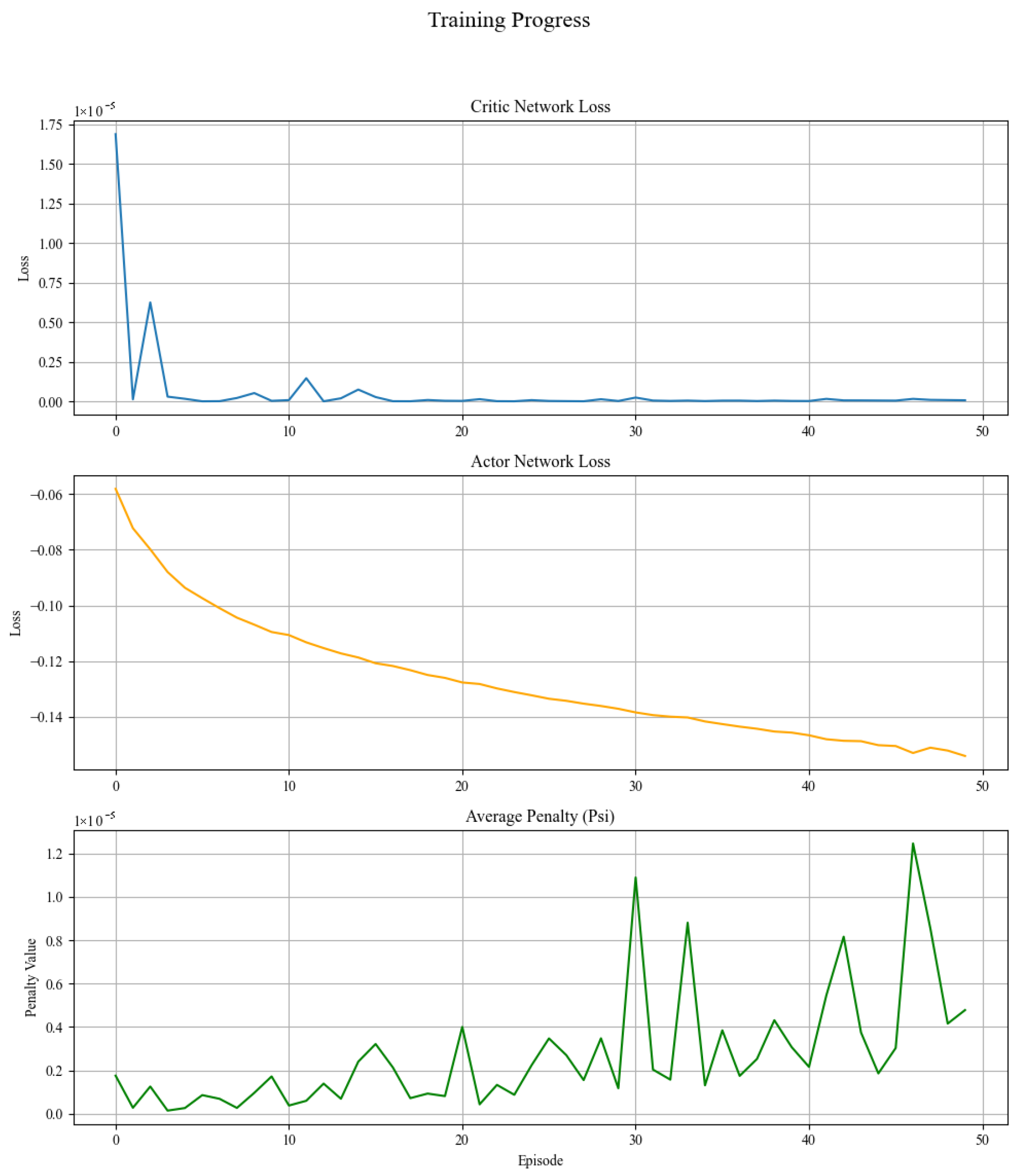
The training diagnostics are summarised in Figure 1. The critic loss decreases monotonically from $1.75\times {10}^{-5}$ to $0.25\times {10}^{-5}$ within 50 episodes, indicating stable convergence of the value network. The actor loss quickly drops to approximately $-0.12$ and remains in a narrow band; the negative value is attributable to the entropy regulariser, confirming simultaneous improvement of expected returns and preservation of exploration. The average penalty term Ψ falls from $1.2$ to about $0.3$ and flattens thereafter, demonstrating that the KL divergence between the alternative and reference measures is effectively controlled.

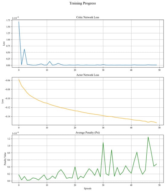
Figure 1. Training progress: critic loss, actor loss, and average penalty.

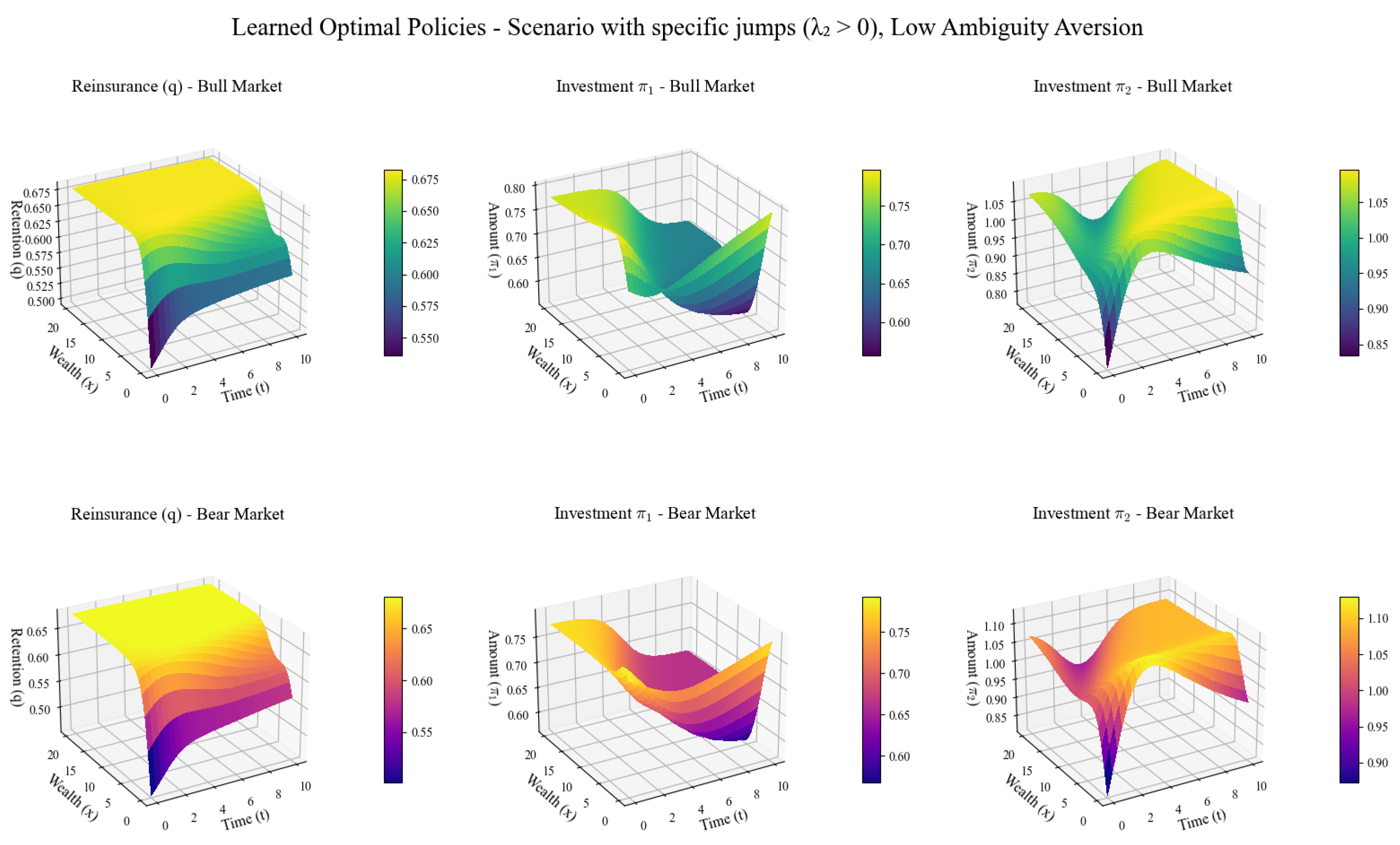
This set of Figure 2 presents the changes in the optimal reinsurance retention ratio (q) and investment strategies for two types of risky assets (${\pi }_1$, ${\pi }_2$) of insurance companies in bull and bear markets over wealth and time.

Figure 2. Optimal strategy.

Despite the bull- and bear-market labels, the three strategy curves differ little overall. The common-shock intensity lies in a low-frequency range, so regime differences are insufficient to amplify tail risk; the relative entropy penalty and entropy regularisation jointly curb extreme policy deviations; moreover, the current surplus is far from the bankruptcy boundary, so capital abundance outweighs the marginal impact of the market regime, driving retention and asset weights to similar levels.

In terms of reinsurance, in a bull market, as time goes by and wealth grows, the retention ratio q gradually increases. Because the market environment is good in a bull market, insurance companies have optimistic profit expectations. After wealth accumulates, their risk-bearing capacity is enhanced, so they are more willing to retain risks to pursue high returns, and the demand for “risk avoidance” through reinsurance decreases. In a bear market, although the retention ratio q also increases with time and wealth, its value is slightly lower. The uncertainty is high in a bear market, and insurance companies face greater operating pressure. Even though the increase in wealth improves their risk-resistance ability, they will not increase the retention ratio as significantly as in a bull market due to caution and will still use reinsurance to diversify part of the risks.

For risky asset investment, in a bull market, the investment in ${\pi }_1$ shows a pattern of being low in the middle and high at both ends as time and wealth change. When wealth is low or high, insurance companies invest in ${\pi }_1$, a high-risk asset, more actively to accumulate wealth quickly and pursue high returns, respectively; when wealth is at an intermediate level, they tend to invest conservatively and reduce the allocation to it. The investment in ${\pi }_2$ increases significantly with the increase in time and wealth because it is relatively stable or has good synergy with insurance business. With the growth of wealth in a bull market, insurance companies are more willing to increase investment in such assets to achieve stable asset appreciation.

In a bear market, the investment in ${\pi }_1$ also has the characteristic of being low in the middle and high at both ends, but the overall level is lower than that in a bull market. The risk is high in a bear market, and insurance companies are more cautious about investing in the high-risk ${\pi }_1$ regardless of the amount of wealth. Although the investment in ${\pi }_2$ increases with the increase in time and wealth, the rate is slower than that in a bull market. Insurance companies will reduce the intensity of investment expansion in such relatively stable assets due to the emphasis on asset safety and liquidity.

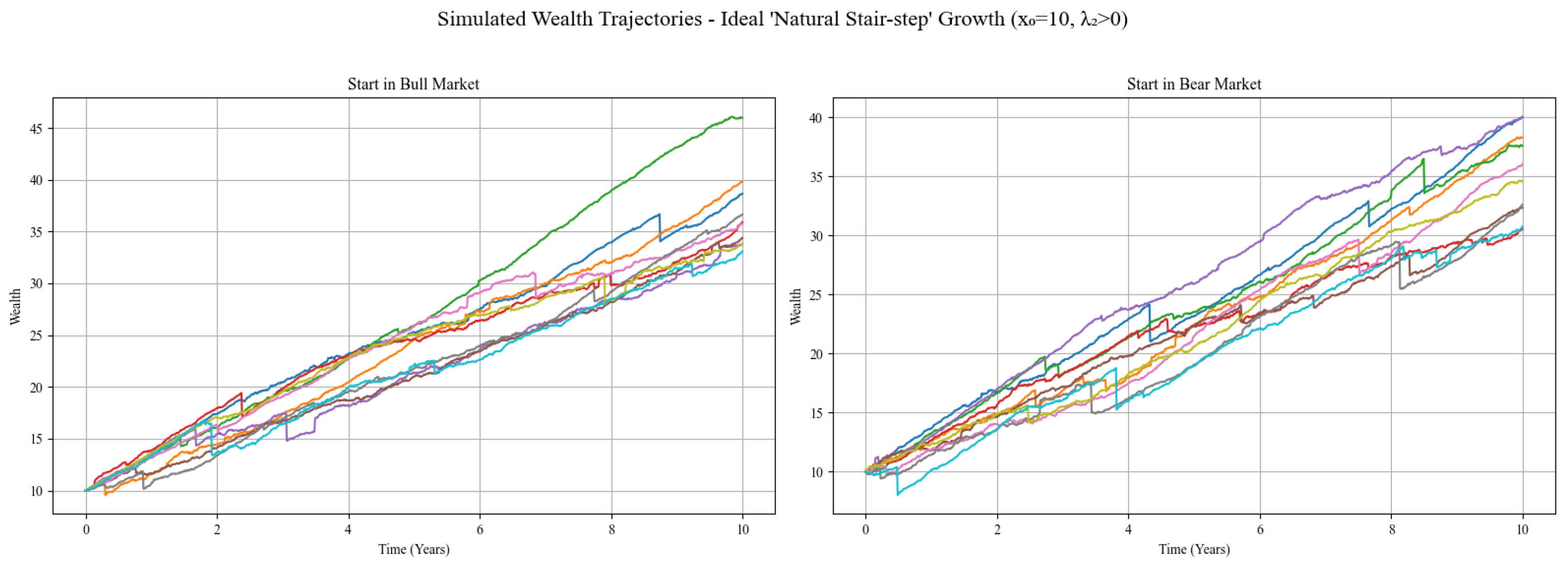
The insurer’s surplus process under the corresponding optimal policy is depicted in Figure 3. Under the robust control framework, the insurer’s surplus trajectory exhibits a “staircase-like” steady growth: the initial market regime has only a limited impact on the path. Regardless of whether the departure point is a bull or bear market, the surplus rapidly converges to a common upward channel within a short period, with the maximum drawdown tightly restricted to approximately five units and the volatility diminishing over time. Throughout the entire planning horizon, the curve moves smoothly upward without severe reversals, demonstrating a strong immunity to model uncertainty and common shocks. Ultimately, the two trajectories almost overlap and stabilize in the 35–40 range, fully embodying the conservative optimization philosophy of “promoting growth through stability” and providing the insurer with a sustainable and resilient capital evolution path.

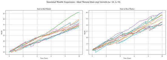
Figure 3. Simulated wealth trajectories.

As a comparison, we consider the standard (non-robust) model by setting the ambiguity-aversion coefficients for all risk sources to extremely large values ${\varphi }_{W_0}={\varphi }_{W_1}={\varphi }_{1i}={\varphi }_{2k,i}={10}^6$ (for each risky asset $k=1,2$). This setting essentially penalizes any deviation from the reference model, thereby degenerating to the traditional expected utility maximization problem.

Figure 4 depicts the optimal strategy and Figure 5 the resulting surplus trajectory when robustness is switched off; in both panels, the decision-maker fully trusts the reference model (all ambiguity-aversion parameters are set to an extremely large value). With no penalty for model deviation, retention and high-risk asset weights are pushed to their upper bounds, producing a steeply rising but oscillatory surplus path whose maximum drawdown quickly exceeds 5 units and whose early slope is highly sensitive to the initial market state (bull or bear).

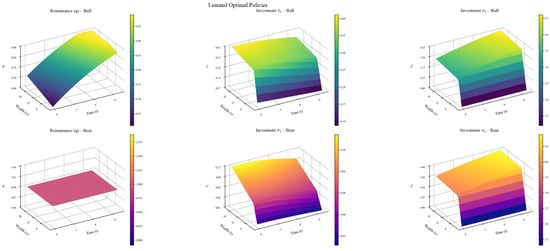
Figure 4. Optimal strategy—non-robust case.

Figure 5. Simulated wealth trajectories—non-robust case.

By contrast, the corresponding plots under the robust regime (Figure 1, Figure 2 and Figure 3) show markedly lower retention, smaller equity exposures, and a smooth, nearly linear surplus accumulation with drawdowns kept below 5 units and rapid mid-horizon convergence regardless of the starting regime.

Hence, while the non-robust design delivers faster upside growth when the model is exact, it does so at the cost of amplified tail volatility and state-dependent instability; the robust alternative trades a modest reduction in early speed for a sustained, regulator-friendly capital channel that remains reliable even under misspecification or large common shocks.

To examine how robust optimal strategies respond to risk, we set ${\lambda }_{2k,i}=0$ and compare the two sets of plots.

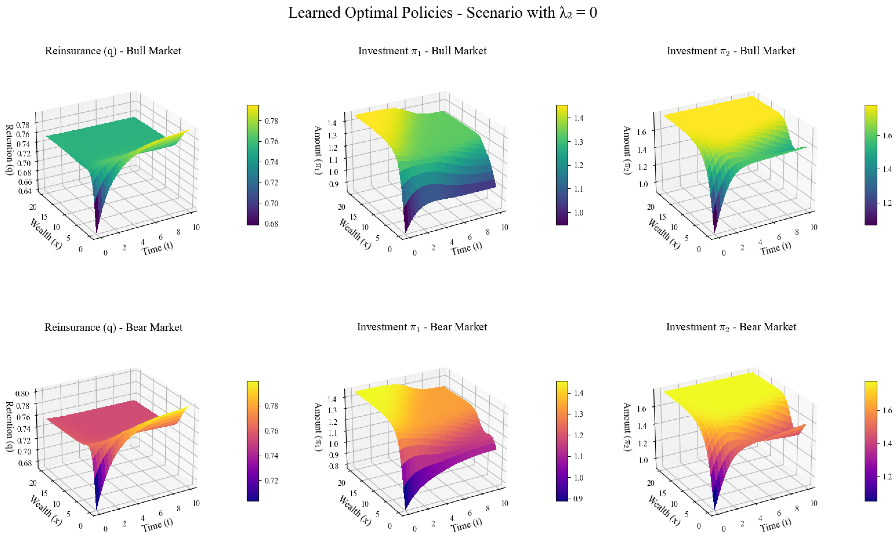
This set of Figure 6 depicts the optimal reinsurance retention ratio (q) and investment strategies for two types of risky assets (${\pi }_1$, ${\pi }_2$) of insurance companies in bull and bear markets as they vary with wealth and time, under the condition that the jump intensity of risky assets ${\lambda }_{2k,i}=0$ (meaning no jumps in risky assets).

Figure 6. Optimal strategy when ${\lambda }_{2k,i}=0$.

Comparing with the scenario where risky assets have jumps (${\lambda }_{2k,i}>0$): in reinsurance, when ${\lambda }_{2k,i}=0$, the retention ratio q is generally higher in both bull and bear markets than when ${\lambda }_{2k,i}>0$, as reduced market risk from no asset jumps boosts insurers’ risk-bearing confidence. For risky asset investment, with ${\lambda }_{2k,i}=0$, investment in both ${\pi }_1$ and ${\pi }_2$ is greater in bull markets, driven by lower asset risk enhancing attractiveness, and also higher in bear markets due to diminished overall risk.

In terms of strategy robustness, when ${\lambda }_{2k,i}=0$, the strategies for reinsurance and risky asset investment show less sensitivity to market fluctuations (bull vs. bear market differences are relatively smaller). The absence of risky asset jumps creates a more stable market environment, making insurers’ decisions less volatile. Conversely, with ${\lambda }_{2k,i}>0$, strategies are more sensitive to market states, as the additional jump risk introduces greater uncertainty, forcing insurers to adjust reinsurance and investment more drastically between bull and bear markets to manage risk.

Model Comparison Insights: Under the condition of ${\lambda }_{2k,i}=0$, the strategic differences between the robust model and the standard model are significantly reduced, indicating that the impact of model uncertainty diminishes in relatively simple market environments. However, in complex environments with ${\lambda }_{2k,i}>0$, the value of the robust model is fully demonstrated, as its strategies can more effectively cope with structural uncertainty.

In summary, ${\lambda }_{2k,i}$ significantly impacts insurers’ decisions: ${\lambda }_{2k,i}=0$ encourages higher reinsurance retention, more aggressive risky asset investments, and more robust strategies, while ${\lambda }_{2k,i}>0$ leads to lower retention, moderated risky asset exposure, and less robust strategies sensitive to market states to balance risk and return.

7. Sensitivity Analysis

To systematically assess the impact of key parameters on the robust optimal reinsurance investment strategy, we conduct single-factor perturbation experiments based on the benchmark parameter set described in Section 6. We select five economically most sensitive parameters and assign each three discrete levels, while keeping all other parameters at their baseline values. The detailed settings are reported in Table 3.

Table 3. Parameter perturbation scheme.

Parameter	Interpretation	Low	Medium	High
${\phi }_{W_0}$	Ambiguity aversion to surplus diffusion	0.5	2.0	4.0
${\phi }_{W_1}$	Ambiguity aversion to market diffusion	0.5	2.0	4.0
${\lambda }_0\left(1\right)$	Common-shock intensity in regime 1	0.05	0.10	0.20
${\lambda }_0\left(2\right)$	Common-shock intensity in regime 2	0.15	0.30	0.45
$\rho$	Correlation between surplus and assets	$-0.6$	$-0.2$	$0.2$

The three panels in Figure 7 depict how the optimal reinsurance ratio $q^{\ast }\left(t\right)$ and the optimal investment weights ${\pi }_1^{\ast }\left(t\right)$, ${\pi }_2^{\ast }\left(t\right)$ react to different levels of ambiguity aversion ${\phi }_{W_0}$ toward surplus diffusion. The curves correspond to ${\phi }_{W_0}=0.5$, $2.0$, and $4.0$.

Figure 7. Sensitivity analysis: ${\phi }_{W_0}$.

Ambiguity aversion to surplus diffusion drives a ${\phi }_{W_0}$ dual conservative mechanism: higher ${\phi }_{W_0}$ simultaneously increases reinsurance coverage and reduces risky positions, with Asset 1 absorbing most of the adjustment. Over the planning horizon, Bayesian updating attenuates but does not eliminate the level differences induced by ${\phi }_{W_0}$.

The three panels in Figure 8 illustrate how the optimal strategy varies with the ambiguity-aversion parameter toward market diffusion ${\phi }_{W_1}$. As ambiguity aversion ${\phi }_{W_1}$ toward market diffusion rises, the optimal reinsurance ratio $q^{\ast }$ only edges up from about $0.50$ to $0.44$, indicating a mild response. In contrast, the weight on Asset 1, ${\pi }_1^{\ast }$, falls sharply from $1.0$ to $0.5$, making it the primary risk-adjustment lever, while the weight on Asset 2, ${\pi }_2^{\ast }$, declines more gently from $0.6$ to $0.4$. All three trajectories drift slowly downward over time, reflecting Bayesian learning: higher ${\phi }_{W_1}$ keeps the strategy conservative for longer, but accumulated data gradually relaxes the initial caution. Overall, ambiguity aversion to market diffusion influences the asset side far more than the liability side, with Asset 1 serving as the key dynamic-hedging instrument.

Figure 8. Sensitivity analysis: ${\phi }_{W_1}$.

As shown in Figure 9, in the bull-market regime (Regime 1), as the common-shock intensity ${\lambda }_0\left(1\right)$ rises from $0.05$ to $0.20$, the optimal reinsurance ratio $q^{\ast }$ edges up only modestly, from about $0.55$ to $0.60$. By contrast, the weight on Asset 1, ${\pi }_1^{\ast }$, drops sharply from $1.3$ to $0.9$, establishing Asset 1 as the primary lever for risk adjustment. The weight on Asset 2, ${\pi }_2^{\ast }$, also declines with increasing ${\lambda }_0\left(1\right)$, but more gently, from roughly $0.6$ to $0.45$. All three trajectories drift slowly downward over time, reflecting Bayesian learning: as more observations accumulate, the tail-probability estimate of a common shock stabilizes, and the initial conservative stance is gradually relaxed. Overall, the common-shock intensity exerts a far stronger influence on the asset side than on the liability side, with Asset 1 s high sensitivity rendering it the core dynamic-hedging instrument.

Figure 9. Sensitivity analysis: ${\lambda }_0\left(1\right)$.

As shown in Figure 10, in the bear-market regime (Regime 2), each increase of $0.15$ in the common-shock intensity ${\lambda }_0\left(2\right)$ raises the optimal reinsurance ratio $q^{\ast }$ by roughly 2-C4 percentage points, while the weight on Asset 1, ${\pi }_1^{\ast }$, falls by about $0.1$; the weight on Asset 2, ${\pi }_2^{\ast }$, adjusts only marginally. All three trajectories drift slowly downward over time, reflecting Bayesian learning: as more observations accumulate, the tail-probability estimate of a common shock stabilizes, and the initial conservative stance is gradually relaxed. Overall, in the bear-market regime the firm relies more heavily on additional reinsurance than on asset reduction to manage tail risk, with Asset 1 remaining the primary lever for dynamic risk control.

Figure 10. Sensitivity analysis: ${\lambda }_0\left(2\right)$.

As shown in Figure 11, when the correlation $\rho$ between surplus and asset returns becomes more positive, tail co-movement risk increases. Consequently, the firm significantly raises the reinsurance ratio $q^{\ast }$ from roughly $0.45$ to $0.65$, while sharply cutting the weight on Asset 1, ${\pi }_1^{\ast }$, from $1.1$ down to $0.6$; the weight on Asset 2, ${\pi }_2^{\ast }$, is adjusted only marginally. All three trajectories drift slowly downward over time, reflecting Bayesian learning: as more observations accumulate, the correlation estimate stabilizes and the initial conservative stance is gradually relaxed. Overall, $\rho$ is the key driver of the “hedge versus reduce” decision, with Asset 1 remaining the primary lever for dynamic risk control.

Figure 11. Sensitivity analysis: $\rho$.

The training curves guarantee numerical reliability, while the policy trajectories illustrate that the algorithm successfully adapts retention and asset allocations to regime-dependent risk profiles. Together, they substantiate the effectiveness of the proposed actor–critic method in solving the high-dimensional HJB system with model uncertainty and jump risk.

8. Conclusions

This paper has presented a comprehensive formulation of the robust optimal reinsurance and portfolio problem with risk interdependence under Markov switching processes. We have derived the wealth process dynamics under both physical and risk-neutral measures, established the corresponding Hamilton–Jacobi–Bellman equation, and provided an explicit form of the relative entropy penalty function that captures model uncertainty from all risk sources. These theoretical contributions provide a solid foundation for developing numerical algorithms, particularly actor–critic reinforcement learning methods, to solve this complex stochastic control problem. Future research directions include extending the framework to incorporate more complex dependence structures, investigating alternative penalty functions, and developing more efficient numerical methods for high-dimensional problems.

References

- Azizpour, S.; Giesecke, K.; Schwenkler, G. Exploring the sources of default clustering. J. Financ. Econ. 2018, 129, 154–183. [Google Scholar] [CrossRef]
- Eisenberg, L.; Noe, T.H. Systemic risk in financial systems. Manag. Sci. 2010, 47, 236–249. [Google Scholar] [CrossRef]
- Zhang, C.B.; Liang, Z.B.; Yuen, K.C. Optimal reinsurance and investment in a Markovian regime-switching economy with delay and common shock. Sci. Sin. (Math.) 2020, 51, 773. [Google Scholar]
- Liang, Z.; Bi, J.; Yuen, K.C.; Zhang, C. Optimal mean-variance reinsurance and investment in a jump-diffusion financial market with common shock dependence. Math. Methods Oper. Res. 2016, 84, 155–181. [Google Scholar] [CrossRef]
- Yuen, K.C.; Liang, Z.B.; Zhou, M. Optimal proportional reinsurance with common shock dependence. Insur. Math. Econ. 2015, 64, 1–13. [Google Scholar] [CrossRef]
- Bauer, D.; Bergmann, D.; Kiesel, R. On the risk-neutral valuation of life insurance contracts with numerical methods in view. Astin Bull. 2010, 40, 65–95. [Google Scholar] [CrossRef]
- Bernard, C.; Vanduffel, S.; Ye, J. Optimal strategies under Omega ratio. Eur. J. Oper. Res. 2019, 275, 755–767. [Google Scholar] [CrossRef]
- Gao, Y.J.; Zhang, Q. Optimal reinsurance and investment problems with delay effects in a thinning dependent risk model. Adv. Appl. Math. 2024, 13, 1523–1535. [Google Scholar] [CrossRef]
- Ximin, R.; Yiqi, Y.; Hui, Z. Asymptotic solution of optimal reinsurance and investment problem with correlation risk for an insurer under the CEV model. Int. J. Control 2023, 96, 840–853. [Google Scholar]
- Zhang, X.; Siu, T.K. On optimal proportional reinsurance and investment in a Markovian regime-switching economy. Acta Math. Sin. Engl. Ser. 2012, 28, 67–82. [Google Scholar] [CrossRef]
- Bouaicha, N.E.H.; Chighoub, F.; Alia, I.; Sohail, A. Conditional LQ Time-Inconsistent Markov-switching Stochastic Optimal Control Problem for Diffusion with Jumps. Mod. Stochastics Theory Appl. 2022, 9, 157–205. [Google Scholar] [CrossRef]
- Lv, S.; Wu, Z.; Xiong, J.; Zhang, X. Robust optimal stopping with regime switching. Optim. Control, 2025; submitted. [Google Scholar]
- Ernst, P.; Mei, H.W. Exact optimal stopping for multidimensional linear switching diffusions. Math. Oper. Res. 2023, 48, 1589–1606. [Google Scholar] [CrossRef]
- Li, L.; Qiu, Z. Time-consistent robust investment-reinsurance strategy with common shock dependence under CEV model. PLoS ONE 2025, 20, e0316649. [Google Scholar] [CrossRef] [PubMed]
- Mu, R.; Ma, S.X.; Zhang, X.R. Robust optimal reinsurance and investment strategies for the insurer and the reinsurer under dependent risk model. Chin. J. Eng. Math. 2024, 41, 245–265. [Google Scholar]
- Guan, G.H.; Liang, Z.X. Robust optimal reinsurance and investment strategies for an AAI with multiple risks. Insur. Math. Econ. 2019, 89, 63–78. [Google Scholar] [CrossRef]
- Wu, H.P.; Zhang, L.M.; Zhao, Q. Alpha-maxmin mean-variance reinsurance-investment strategy under negative risk dependence between two markets. J. Comput. Appl. Math. 2025, 463, 116350. [Google Scholar] [CrossRef]
- Zhang, Q.; Wu, L.J. Robust optimal proportional reinsurance and investment problem for an insurer with delay and dependent risks. Commun. Stat. C Theory Methods 2024, 53, 34–65. [Google Scholar] [CrossRef]
- Zhao, H.; Shen, Y.; Zeng, Y. Time-consistent investment-reinsurance strategy for mean-variance insurers with a defaultable security. J. Math. Anal. Appl. 2016, 437, 1036–1057. [Google Scholar] [CrossRef]
- Boyle, P.; Tian, W. Portfolio Management with Constraints. Math. Financ. 2007, 17, 319–343. [Google Scholar] [CrossRef]
- Gao, J.; Zhou, K.; Li, D.; Cao, X. Dynamic Mean-LPM and Mean-CVaR Portfolio Optimization in Continuous-time. Siam J. Control Optim. 2017, 55, 1377–1397. [Google Scholar] [CrossRef]
- Allan, A.L.; Cuchiero, C.; Liu, C.; Prömel, D.J. Model-free Portfolio Theory: A Rough Path Approach. Math. Financ. 2023, 33, 709–765. [Google Scholar] [CrossRef]
- Denardo, E.V. Contraction mappings in the theory underlying dynamic programming. SIAM Rev. 1967, 9, 165–177. [Google Scholar] [CrossRef]
- Oksendal, B. Stochastic Differential Equations: An Introduction with Applications; Springer-Verlag: Berlin/Heidelberg, Germany, 2003. [Google Scholar]
- Jia, Y.; Zhou, X.Y. Policy Gradient and Actor-Critic Learning in Continuous Time and Space: Theory and Algorithms. Soc. Sci. Res. Netw. 2022, 23, 1–50. [Google Scholar] [CrossRef]
- Zhou, M.; Han, J.; Lu, J. Actor-critic method for high dimensional static Hamilton-Jacobi-Bellman partial differential equations based on neural networks. SIAM J. Sci. Comput. 2021, 43, A4043–A4066. [Google Scholar] [CrossRef]
- Jin, Z.Y.; Yang, H.Z.; Yin, G. A hybrid deep learning method for optimal insurance strategies: Algorithms and convergence analysis. Insur. Math. Econ. 2021, 96, 262–275. [Google Scholar] [CrossRef]
- Xiao, H.S.; Wen, Y.J.; Wang, Y. Research on portfolio optimization based on deep reinforcement learning. Stat. Appl. 2025, 14, 229–240. [Google Scholar] [CrossRef]
- Ou, P.; Lu, X.G. Reinsurance and investment problems based on actor-critic reinforcement learning. Adv. Appl. Math. 2025, 14, 135–142. [Google Scholar] [CrossRef]
- Maenhout, P.J. Robust Portfolio Rules and Asset Pricing. Rev. Financ. Stud. 2004, 17, 951–983. [Google Scholar] [CrossRef]
Disclaimer/Publisher’s Note: The statements, opinions and data contained in all publications are solely those of the individual author(s) and contributor(s) and not of MDPI and/or the editor(s). MDPI and/or the editor(s) disclaim responsibility for any injury to people or property resulting from any ideas, methods, instructions or products referred to in the content. |
© 2025 by the authors. Licensee MDPI, Basel, Switzerland. This article is an open access article distributed under the terms and conditions of the Creative Commons Attribution (CC BY) license (https://creativecommons.org/licenses/by/4.0/).