Abstract
This paper investigates the problem of data-driven optimal preview repetitive control of linear discrete-time systems. Firstly, by integrating prior information into the preview time domain, an augmented state-space system is established. Secondly, the original output tracking problem is mathematically reconstructed and transformed into the optimization problem form of a linear quadratic tracking (LQR). Furthermore, a Q-function-based iterative algorithm is designed to dynamically calculate the optimal tracking control gain based solely on online measurable data. This method has a dual-breakthrough feature: it neither requires prior knowledge of system dynamics nor provides an initial stable controller. Finally, the superiority of the proposed scheme is verified through numerical simulation experiments.
MSC:
93D21
1. Introduction
In practical control system applications, there is often a situation where the system tracks a specific periodic signal. Repetitive control (RC) is a high-precision control method that tracks a reference signal with a known period [1]. Preview control (PC) is a control method that improves the performance of closed-loop systems by utilizing known future information from target signals or interference signals [2]. The combination of PC and RC, known as preview repetitive control [3,4] (PRC), was first developed in the early 1990s. It utilizes both the internal model compensation mechanism of repetitive learning and the compensation of preview information; thus, it can significantly improve the control performance of closed-loop systems.
Recently, a great deal of research has been devoted to the theory and applications of PRC, and various structures and algorithms have been devised [5,6,7,8]. In [5], a design method of discrete-time sliding-mode preview repetitive servo systems was proposed. Using a parameter-dependent Lyapunov function method and linear matrix inequality (LMI) techniques, a robust guaranteed-cost PRC law was proposed in [6]. Based on the optimal control theory, the problem of optimal PRC for continuous-time linear systems was investigated in [7] by solving the algebraic Riccati equation (ARE). Using a two-dimensional model approach, observer-based PRC for uncertain discrete-time systems was studied in [8]. In [9], a discrete-time PRC scheme was proposed for linear discrete-time periodic systems. To compensate for unknown external disturbances, the problem of PRC with equivalent-input disturbance (EID) for uncertain continuous-time systems was presented in [10]. The problem of Padé approximation-based optimal PRC with EID was proposed in [11]. In [12], the PRC for discrete-time linear parameter-varying systems with a time-varying delay was investigated. However, the above results depend on a perfect understanding of the system model.
In model driven-based control, a mathematical model is first established and the controller is then designed based on this model [13,14]. The inherent problem of system modeling is the motivation for research in the field of data-driven control (DDC) technology [15,16]. An approach of designing an optimal preview output tracking controller using online measurable data and a Q-function-based iteration algorithm was developed [17]. A data-driven framework to control a complex network optimally and without any knowledge of the network dynamics was develop in [18]. The fault-tolerant consensus control problem for a general class of linear continuous-time multi-agent systems (MASs) was considered in [19]. In [20], the problem of the decoupled eata-based optimal control policy for a nonlinear stochastic systems was addressed. In [21], a data-based iteration learning control for multiphase batch processes was investigated. A data-based approach to linear quadratic tracking (LQT) control design was presented in [22]. In [23], a novel adaptive dynamic programming-based learning algorithm was proposed by only accessing the input and output data to solve the LQT problem. In [24], a robust data-driven finite-horizon linear quadratic regulator control problem of unknown linear time-invariant systems was addressed. DDC-based optimal tracking control for systems in the presence of external disturbance was presented in [25,26].
Note that the mechanism model with system matrices and order needs to be known in existing PC/RC studies. Actually, many practical plants are hard to model, particularly for the complicated modern control systems and complex networks [27]. On the other hand, the above studies do not reflect the research interests in data-driven PC and RC compensation information. These observations inspire our current study. In this paper, we investigate the problem of data-driven preview repetitive control (DD-PRC) of linear discrete-time systems. The main contributions of this paper are summarized as follows: (i) By taking advantage of the preview information of the desired tracking signal as well as the periodic learning ability of repetitive control, the original control problem is converted to an LQT one under an augmented state-space model. (ii) In order to solve the DDC-based LQT problem, a Q-function-based iterative algorithm is then designed to dynamically calculate the optimal tracking control gain instead of solving the ARE.
2. Problem Formulation
Consider a discrete-time linear system given by
where is the system state, is the measurement output, and is the control input. , and C are the corresponding appropriate dimensional matrices.
The configuration of the data-driven PRC system is shown in Figure 1, where is the controlled plant as described in System (1). denotes the constant reference trajectory signal with a period of L. is the basic repetitive control block, and is the output of the repetitive controller and is given by
where is the tracking error.
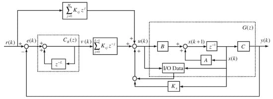
Figure 1.
Configuration of data-driven PRC system.
The following assumptions are needed for System (1).
Assumption 1.
Assume that , and C satisfy both controllable and observable.
Assumption 2.
The preview length of the reference trajectory signal is limited to M (). That is, at the current moment k, the current value of and the M-step future values are available. Additionally, it is assumed that the future values beyond the reference trajectory forward range L are set to 0, i.e., .
Remark 1.
Note that Assumption 1 is a necessary assumption for the optimal state feedback control, while Assumption 2 is a standard working hypothesis introduced to facilitate the PC mathematical development [2,3,4]. It indicates that the reference signal’s values are known in the actual system for a certain time period, during which the reference signal exceeds the preview length, and the impact is very small.
The objective of this paper is to design a DD-PRC law with the form of
where and are the gains of the repetitive controller and the preview compensator, respectively, and is the gain of the feedback controller, such that the system output tracks the reference signal and the quadratic cost function
is minimized subject to system (1), where and R are symmetric positive definite and semi-positive definite symmetric matrices, respectively, and
Now, define the following L-order difference operator:
Substituting (5) into System (1) yields
Introducing the state vector
Therefore,
where
Since M-step future values are available, a new state vector can be defined as
Combining Equations (8) and (9) yields
where
With these definitions, the performance index (4) can be rewritten as
where, .
Thus, the control problem associated with Discrete System (1) under Performance Index (4) is converted into an optimal LQT control problem of the Augmented System (10), subject to Performance Index (11).
Hence, if the optimal controller subject to (10) and (11) is solved, then the DD-PRC law (13) will be derived. In fact, using (5) and (12), we can find that
It can be seen that the above control law consists of three terms. The first term represents RC, which is used to eliminate the steady-state tracking error. The second term describes the state-feedback control, which is used to guarantee the stability of closed-loop system. The third term denotes the preview action, which is used to improve the transient response of systems. The combination of these three terms can achieve the satisfactory tracking performance.
3. Data-Driven PRC Law Design
It has been shown in [28] that the optimal controller can be obtained if we can find a unique positive definite solution of the following algebraic Riccati equation (ARE):
Then, we can obtain the optimal controller:
where
This problem can be solved using the iterative algorithm [17,28] to approximate the solution of ARE (14), which is given as Algorithm 1 for comparison in the next section.
| Algorithm 1 Iterative algorithm for solving K |
|
Note that the above iterative algorithm, Algorithm 1, is essentially model-based. In this section, we will develop a model-free control approach by using online input and output data.
For the LQT problem, we define the following cost function:
whose optimal value can be parameterized as
Using the well-known Bellman equation, we get
where can be viewed as the gain from reinforcement learning, and the corresponding function can be viewed as the cost function.
Define a Q-function, also known as action value function , given by
From (21), it can be observed that this Q-function describes the performance associated with the state–action pair
For the proposed optimal controller , it can be derived from Equations (20) and (21) that and therefore the Q-function also has a corresponding Bellman formation:
From the optimality of Bellman’s formula, the optimal value function and the optimal controller is given by
By solving , we can obtain
If P is the only positive definite solution obtained from the ARE (14), then , which is equal to the gain of the optimal LQT control.
The Q-learning scheme generates the sequences , and can converge to , , respectively, which has been proven in [29]. It is worth pointing out that this Q-learning scheme requires a priori information of system dynamics and an initially stabilizing control gain. To overcome this drawback, in the following section, based on the Q-function value, a data-driven based algorithm will be developed to obtain the optimal control gain.
To implement the iterative algorithm, the iterative Q-function is denoted as
where
In the following, for computational simplicity, the Kronecker product is introduced to convert into a vector representation. Note that
where , ⊗ is the Kronecker product, and is the vector formed by stacking the columns of matrix Therefore, it follows from (31) that
where
For a given positive integer N, denote and . Then by collecting sample data, we have
By using the least squares method, unknown parameter vectors can be calculated by
Remark 2.
Note that the matrix Ξ is used in each iteration, so the measured data can be fully utilized. Thus, we should collect enough data so that the rank of Ξ is equal to the unknown independent parameter possessed by the vector G, ensuring that Equation (37) has a unique solution. The rank condition is bound up with the persistence of excitation or exploratory signals, which ensures that enough information about system dynamics is collected.
On the other hand, the convergence of the least squares solution depends on the convexity of the problem and the initial conditions of the iterative algorithm. When the least squares problem is convex, the iterative method usually converges to the optimal solution. If it is a non-convex problem, there may be convergence difficulties. By adding constraints, such as adjusting the threshold and the maximum number of iterations, the convergence of the non-convex problem can be improved.
Now, a data-driven algorithm is developed for solving K in (30), referred to as Algorithm 2.
| Algorithm 2 Data-driven algorithm for solving K |
|
Remark 3.
Algorithm 2 is a DDC method. The algorithm is implemented using past input, output, and preview reference data measured by the system, which does not require any priori knowledge of the system dynamics.
Remark 4.
Algorithm 2 is a DD-PRC algorithm for linear discrete-time systems. According to the data-driven robust fault-tolerant control studied in [15], Algorithm 2 can be extended to nonlinear systems by using the Markov parameter sequence identification method.
4. Simulation Results
In this section, the effectiveness of the proposed algorithm is verified by a simulation example.
Consider the following linear discrete system:
where . Assume that the reference signal with period is given by
The performance index is denoted as (4) with and . Set the preview length to .
By some calculation, we can find that is controllable and is observable. By solving the ARE (14), we obtain the optimal control gain:
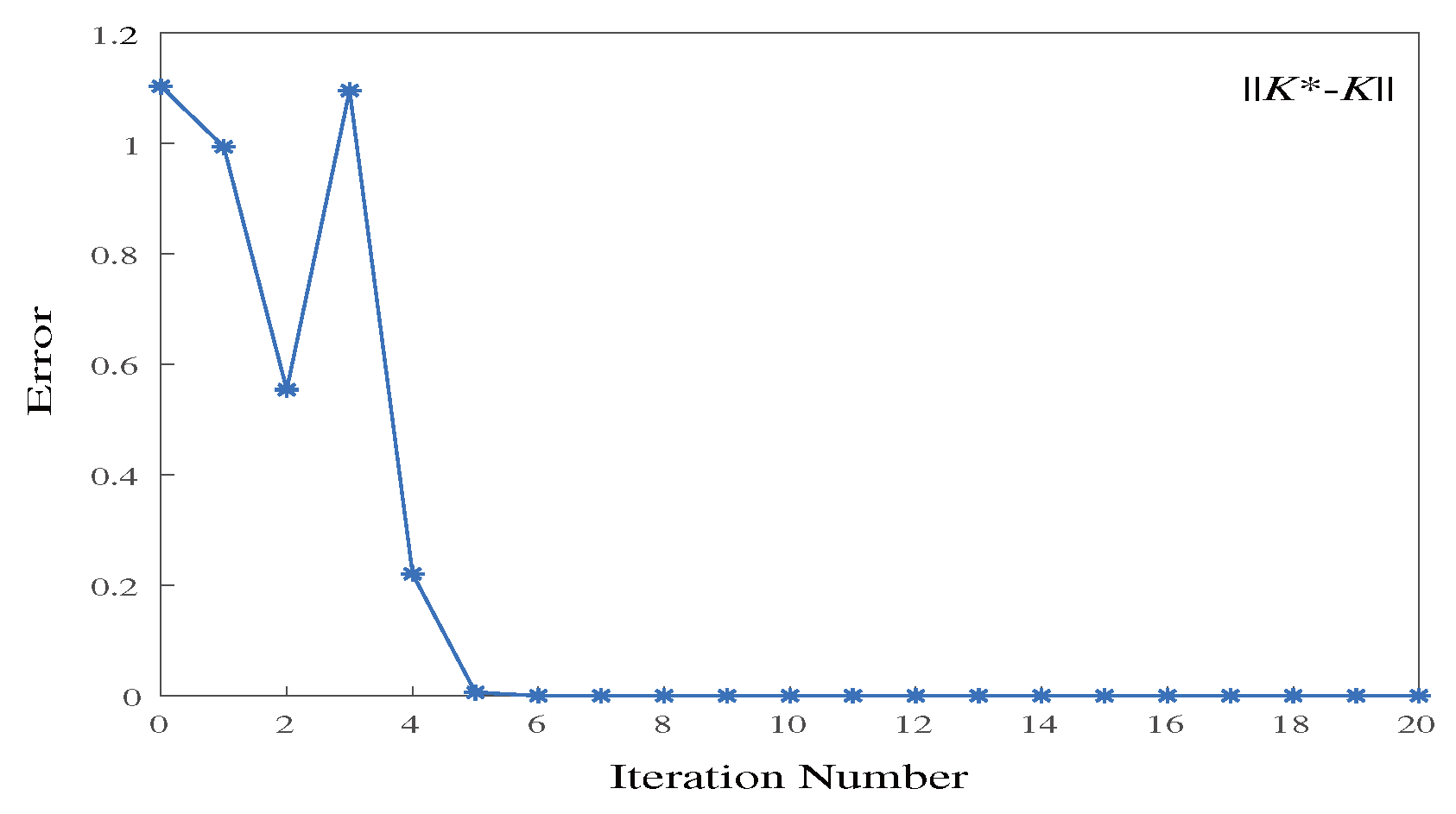
Set Using Algorithm 1 to solve for K, at th iteration, we get the optimal control gain . While using Algorithm 2 to solve for K, at th iteration, we get
Altough the obtained by Algorithm 1 is more accurate, it depends on the prior information of system matrices. On account of the inevitability of parametric variations or unmodeled dynamics, it is usually hard to obtain the perfect model of a physical system. In the next section, we will use to perform the simulation.
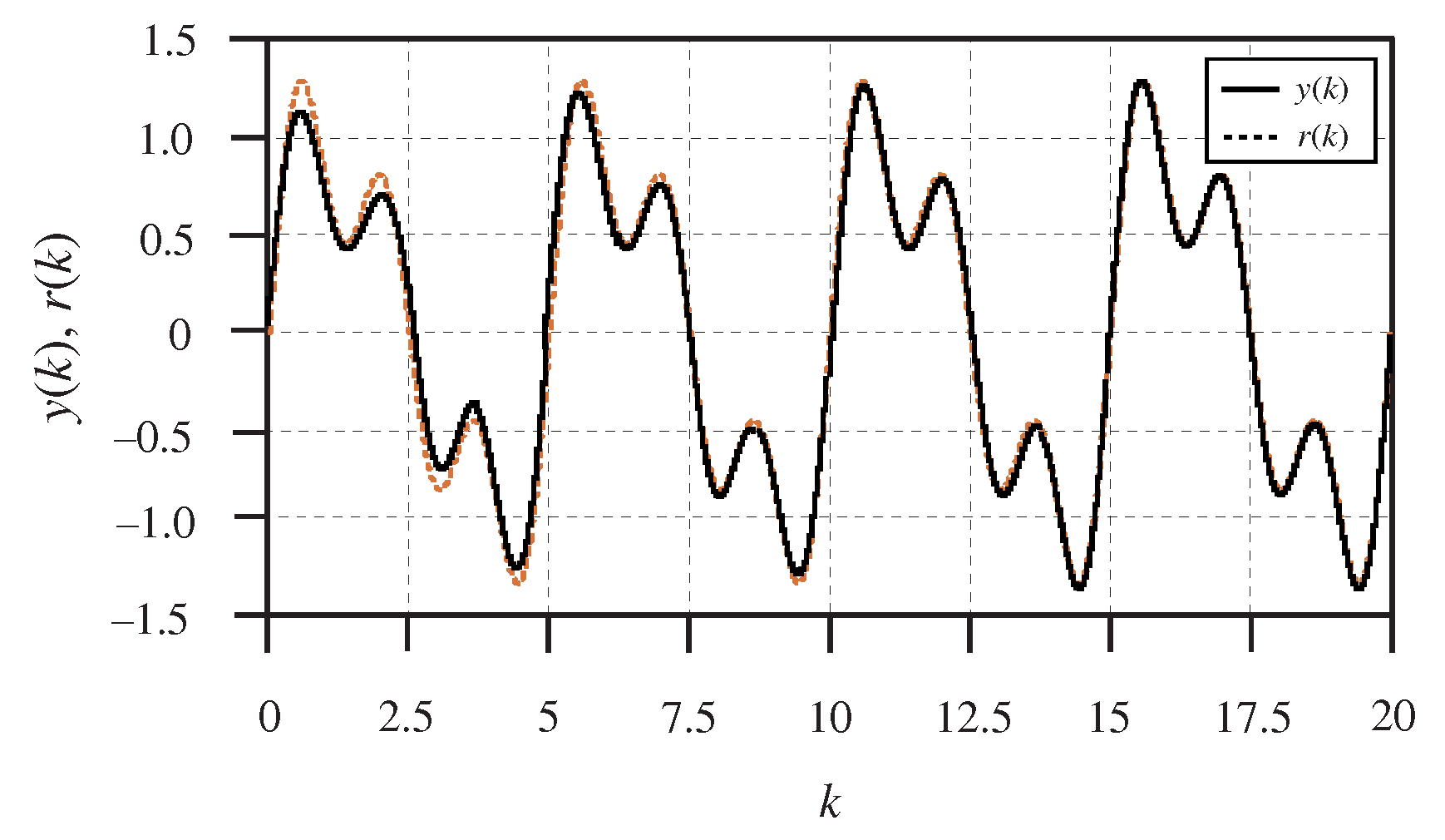
The simulation results are given in Figure 2, Figure 3 and Figure 4. Figure 2 shows the norm of the difference between the controller gain K and the optimal tracking controller gain during the iteration process. Figure 3 shows the system output and the reference signal under the data-driven PRC law (13) at th iteration. The tracking error is depicted in Figure 4. It can be seen from these Figures that the data-based algorithm proposed in this paper is capable of realizing tracking control tasks successfully.
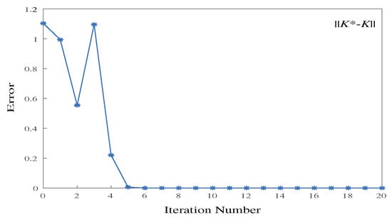
Figure 2.
The values of .
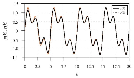
Figure 3.
The system output and the reference signal.
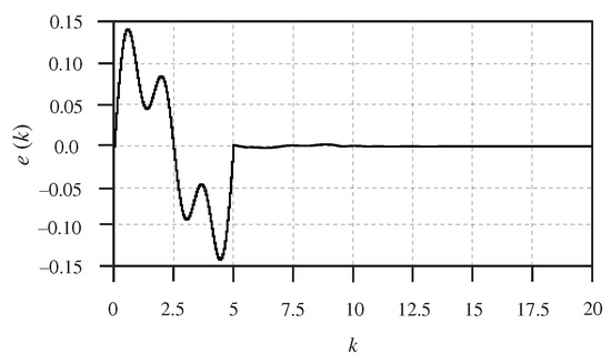
Figure 4.
The tracking error.
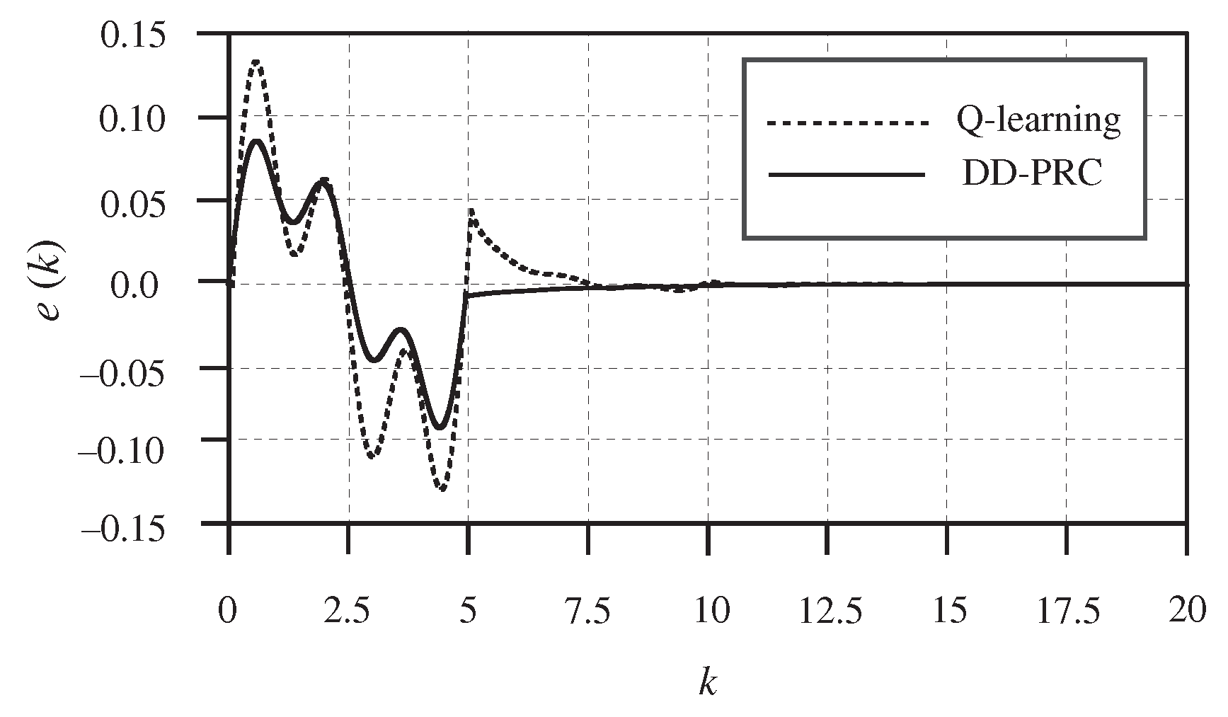
To test the robustness, we compared the simulation results between our approach and the Q-learning method proposed in [24]. Add a disturbance signal to the input signal of the control system. The simulation result is shown in Figure 5. It can be seen that both the outputs can track the reference signal accurately. However, DD-PRC can more effectively reduce the tracking error. The reason is the combination of preview and repetitive learning.

Figure 5.
The tracking errors under different controllers.
Furthermore, Gaussian white noise is also added to the disturbance term . Noise with varying variances is selected, and 50 Monte Carlo experiments are conducted for each variance level. This process yields the mean and standard deviation (SD) of the sum square error (SSE) for the two controllers under different noise intensities, as presented in Table 1. As is evident from Table 1, we can conclude that the DD-PRC method has superior anti-interference ability compared to the Q-learning method proposed in [24].

Table 1.
The comparison of SSE with different controller.
5. Conclusions
In this paper, a data-based PRC algorithm for addressing the tracking control problem of linear discrete-time systems is designed. The algorithm transforms the system’s optimal tracking problem into a linear quadratic regulation problem. A data-driven approach is proposed without relying on system dynamics, enabling the resolution of LQT using solely measured input, output, and reference trajectory data. Finally, MATLAB R2022a simulation results demonstrate that the proposed data-driven PRC algorithm exhibits satisfactory tracking performance.
Author Contributions
Methodology, X.-L.L.; Software, Q.-L.W.; Formal analysis, X.-L.L.; Data curation, Q.-L.W. All authors have read and agreed to the published version of the manuscript.
Funding
This research received no external funding.
Data Availability Statement
The original contributions presented in this study are included in the article. Further inquiries can be directed at the corresponding author.
Conflicts of Interest
The authors declare no conflicts of interest.
References
- Hara, S.; Yamamoto, Y.; Omata, T.; Nakano, M. Repetitive control system: A new type servo system for periodic exogenous signals. IEEE Trans. Autom. Control 1988, 33, 659–668. [Google Scholar] [CrossRef]
- Hać, A. Optimal linear preview control of active vehicle suspension. Veh. Syst. Dyn. 1992, 21, 167–195. [Google Scholar] [CrossRef]
- Nakamura, H. Preview repetitive control considering delays in manipulation and detection. J. Autom. Control 1994, 30, 871–873. [Google Scholar]
- Egami, T. A design of low-degree optimal preview repetitive control system. Trans. Soc. Instrum. Control Eng. 1999, 35, 297–299. [Google Scholar] [CrossRef][Green Version]
- Tadashi, S.; Tadashi, E.; Takeshi, T. Design of discrete-time sliding-mode preview-repetitive control systems. Trans. Inst. Syst. Control Inf. Eng. 2005, 18, 312–321. [Google Scholar]
- Lan, Y.H.; Xia, J.J.; Shi, Y.X. Robust guaranteed-cost preview repetitive control for polytopic uncertain discrete-time systems. Algorithms 2019, 12, 20. [Google Scholar] [CrossRef]
- Lan, Y.H.; He, J.L.; Li, P.; She, J.H. Optimal preview repetitive control with application to permanent magnet synchronous motor drive system. J. Franklin Inst. 2020, 357, 10194–10210. [Google Scholar] [CrossRef]
- Li, L. Observer-based preview repetitive control for uncertain discrete-time systems. Int. J. Robust Nonlinear Control 2021, 31, 1103–1121. [Google Scholar] [CrossRef]
- Li, L.; Lu, Y. Preview repetitive control for linear discrete-time periodic systems. Int. J. Adapt. Control Signal Process. 2022, 36, 412–428. [Google Scholar] [CrossRef]
- Lan, Y.H.; Zhao, J.Y. Design of a preview repetitive control with equivalent-input-disturbance system based on a continuous-discrete 2D model. J. Franklin Inst. 2023, 360, 1884–1903. [Google Scholar] [CrossRef]
- Lan, Y.H.; Zhao, J.Y. Improving track performance by combining padé-approximation-based preview repetitive control and equivalent-input-disturbance. J. Electr. Eng. Technol. 2024, 19, 3781–3794. [Google Scholar] [CrossRef]
- Li, L.; Lu, Y.; Meng, X. Preview repetitive control for discrete-time linear parameter-varying systems with a time-varying delay. Trans. Inst. Meas. Control 2025, 01423312241300756. [Google Scholar] [CrossRef]
- Rguigui, H.; Elghribi, M. Practical stabilization for a class of tempered fractional-order nonlinear fuzzy systems. Asian J. Control 2025. [Google Scholar] [CrossRef]
- Chen, Y.; Wang, H.; Wang, X. Precision fixed-time formation control for multi-AUV systems with full state constraints. Mathematics 2025, 13, 1451. [Google Scholar] [CrossRef]
- Han, K.Z.; Feng, J. Data driven robust fault tolerant linear quadratic preview control of discrete-time linear systems with completely unknown dynamics. Int. J. Control 2019, 94, 49–59. [Google Scholar] [CrossRef]
- Huang, J.W.; Gao, J.W. How could data integrate with control? A review on data-based control strategy. Int. J. Dyn. Control 2020, 8, 1189–1199. [Google Scholar] [CrossRef]
- Liu, Z.Y.; Wu, H.N. Data-driven optimal preview output tracking of linear discrete-time systems. In Proceedings of the 38th Chinese Control Conference, Guangzhou, China, 27–30 July 2019; pp. 1973–1978. [Google Scholar]
- Baggio, G.; Bassett, D.S.; Pasqualetti, F. Data-driven control of complex networks. Nat. Commun. 2021, 12, 1429. [Google Scholar] [CrossRef]
- Gao, C.; Wang, Z.; He, X.; Yue, D. Sampled-data-based fault-tolerant consensus control for multi-agent systems: A data privacy preserving scheme. Automatica 2021, 133, 109847. [Google Scholar] [CrossRef]
- Wang, R.; Parunandi, K.S.; Yu, D.; Kalathil, D.; Chakravorty, S. Decoupled data-based approach for learning to control nonlinear dynamical Systems. IEEE Trans. Autom. Control 2022, 67, 3582–3589. [Google Scholar] [CrossRef]
- Geng, Y.; Ruan, X.; Yang, X.; Zhou, Q. Data-based iterative learning control for multiphase batch processes. Asian J. Control 2023, 25, 1392–1406. [Google Scholar] [CrossRef]
- Yan, Y.; Bao, J.; Huang, B. An approach to data-based linear quadratic optimal control. IEEE Control Syst. Lett. 2024, 8, 1120–1125. [Google Scholar] [CrossRef]
- Xie, K.; Zheng, Y.; Jiang, Y.; Lan, W.; Yu, X. Optimal dynamic output feedback control of unknown linear continuous-time systems by adaptive dynamic programming. Automatica 2024, 163, 111601. [Google Scholar] [CrossRef]
- Wang, L.; Liu, W.; Li, Y.; Sun, J.; Wang, G. Data-based online linear quadratic gaussian control from noisy data. Int. J. Robust Nonlinear Control 2025. [Google Scholar] [CrossRef]
- Dao, P.N.; Dao, Q.H. H∞ tracking control for perturbed discrete-time systems using On/Off policy Q-learning algorithms. Chaos Solitons Fractals 2025, 197, 116459. [Google Scholar] [CrossRef]
- Peyman, A.; Aref, S.; Mehdi, R. Data-based H∞ optimal tracking control of completely unknown linear systems under input constraints. IET Control Theory Appl. 2025, 19, 70022. [Google Scholar]
- Yu, T.; Zhao, Y.; Wang, J.; Liu, J. Event-triggered sliding mode control for switched genetic regulatory networks with persistent dwell time. Nonlinear Anal. Hybrid Syst. 2022, 44, 101135. [Google Scholar] [CrossRef]
- Kiumarsi, B.; Lewis, F.L.; Naghibi-Sistani, M.B.; Karimpour, A. Optimal tracking control of unknown discrete-time linear systems using input-output measured data. IEEE Trans. Cybern. 2015, 45, 2770–2779. [Google Scholar] [CrossRef] [PubMed]
- Song, S.; Zhu, M.; Dai, X.; Gong, D. Model-free optimal tracking control of nonlinear input-affine discrete-time systems via an iterative deterministic Q-learning algorithm. IEEE Trans. Neural Netw. Learn. Syst. 2022, 35, 999–1012. [Google Scholar] [CrossRef]
Disclaimer/Publisher’s Note: The statements, opinions and data contained in all publications are solely those of the individual author(s) and contributor(s) and not of MDPI and/or the editor(s). MDPI and/or the editor(s) disclaim responsibility for any injury to people or property resulting from any ideas, methods, instructions or products referred to in the content. |
© 2025 by the authors. Licensee MDPI, Basel, Switzerland. This article is an open access article distributed under the terms and conditions of the Creative Commons Attribution (CC BY) license (https://creativecommons.org/licenses/by/4.0/).


