A Study on the Semi-Discrete KP Equation: Bilinear Bäcklund Transformation, Lax Pair and Periodic Wave Solutions

Abstract

In this paper, we investigate the integrability and solution structure of the semi-discrete KP equation. A bilinear Bäcklund transformation, Lax pair, and nonlinear superposition formula are systematically derived, establishing the integrability of the system. Furthermore, one- and two-periodic wave solutions are constructed using Hirota’s method combined with Riemann theta functions. By means of a rigorous limiting procedure, the asymptotic behavior of the periodic wave solutions is analyzed, and the connection between periodic wave and soliton solutions is established. These results not only enrich the solution structure of the semi-discrete KP equation but also provide new perspectives on periodic phenomena in discrete integrable systems.

1. Introduction

The investigation of integrable systems represents a cornerstone of mathematical physics, forging deep connections between pure mathematics and nonlinear physical phenomena. In recent years, discrete integrable systems have gained considerable attention. Discrete integrable systems arise naturally in fields such as statistical mechanics, quantum theory, and hydrodynamics [1,2,3,4]. Their integrability is of particular value for numerical computation [5,6,7,8,9,10,11,12], as it ensures structure-preserving properties in algorithms, allowing the exact conservation of key physical quantities. The Hirota–Miwa equation [13,14], also known as the discrete Kadomtsev–Petviashvili (KP) equation, is a master model in the theory of discrete integrable systems. It provides a unified framework for understanding various integrable hierarchies and serves as a generating function for numerous prominent integrable equations, including the KP equation, two-dimensional Toda lattice, sine-Gordon equation, and Benjamin–Ono equation [15,16].

The Hirota-Miwa equation is expressed in the following bilinear form

$$a_1(a_2-a_3){\tau }_1{\tau }_{23}+a_2(a_3-a_1){\tau }_2{\tau }_{31}+a_3(a_1-a_2){\tau }_3{\tau }_{12}=0$$

where $\tau$ is a function of the discrete variables $n_1$, $n_2$ and $n_3$, where ${\tau }_1=\tau (n_1+1,n_2,n_3)$, ${\tau }_{23}=\tau (n_1,n_2+1,n_3+1)$ and similarly for the other indices; and $a_1$, $a_2$, and $a_3$ are spacing parameters in the three directions corresponding to $n_1$, $n_2$, and $n_3$. A semi-discrete KP (sdKP) equation [13] was obtained by taking a continuous limit from the Hirota–Miwa equation, and its bilinear form is

$$(a_1-a_2)({\tau }_1{\tau }_2-{\tau }_{12}\tau )+a_1{a}_2{D}_x{\tau }_1·{\tau }_2=0,$$

(1)

in which $\tau$ comes to a function of the continuous variable x and discrete variables $n_1$, $n_2$. Here, Hirota’s bilinear operator is defined by [17]

$$D_{x}f(x,t)·g(x,t)={\displaystyle \frac{\partial f(x,t)}{\partial x}}g(x,t)-f(x,t){\displaystyle \frac{\partial g(x,t)}{\partial x}}.$$

The above equation can be expressed as the equivalent form

$$(a_1{a}_2{D}_x{\mathrm{e}}^{{\displaystyle \frac{D_{n_1}-D_{n_2}}{2}}}-(a_1-a_2){\mathrm{e}}^{{\displaystyle \frac{D_{n_1}+D_{n_2}}{2}}}+(a_1-a_2){\mathrm{e}}^{{\displaystyle \frac{D_{n_1}-D_{n_2}}{2}}})\tau ·\tau =0,$$

(2)

where Hirota’s difference operator is defined as follows

$${\mathrm{e}}^{\delta D_{n_j}}f\left(n_j\right)·g\left(n_j\right)=f(n_j+\delta )g(n_j-\delta ),j=1,2.$$

Through the dependent variable transformation $G=-{\left(\ln \tau \right)}_x$, the bilinear sdKP Equation (2) is rewritten in nonlinear form

$$a_1{a}_2[(G_1-G_2)(G_{12}-G_1-G_2+G)+(G_{1x}-G_{2x})]=(a_1-a_2)(G_{12}-G_1-G_2+G).$$

(3)

Determinant solutions, including soliton solutions of Equation (3), were obtained in Ref. [18]. In addition, periodic solutions are of fundamental importance in nonlinear science, as they provide exact descriptions of coherent wave structures and serve as prototypical models for understanding nonlinear dynamics, modulational stability, and energy localization in physical systems. Nakamura presented a direct approach [19,20] to obtain multi-periodic wave solutions of nonlinear integrable equations by using Riemann theta functions [21]. Research on periodic wave solutions has focused mainly on continuous soliton equations in (1 + 1) and (2 + 1) dimensions [22,23,24,25,26,27,28,29,30], with significantly fewer results available for discrete soliton equations [31,32,33,34,35]. The purpose of this paper is to construct periodic solutions of the semi-discrete KP equation and analyze their connection with soliton solutions. This paper is organized as follows. In Section 2, Bäcklund transformations, Lax pair and the nonlinear superposition formula are derived. In Section 3 and Section 4, the one-periodic solution and the two-periodic solution are obtained, and the asymptotic properties are discussed. Finally, the conclusion and discussions are given in Section 5.

2. Bilinear Bäcklund Transformation and the Nonlinear Superposition Formula

The bilinear sdKP Equation (2) has the following bilinear Bäcklund transformation (BT) [36]

$$\begin{array}{ccc}& & D_x\tau ·\tilde{\tau }=\theta \tau ·\tilde{\tau }+\lambda (a_1-a_2){\mathrm{e}}^{D_{n_2}}\tau ·\tilde{\tau }\hfill \end{array}$$

(4)

$$\begin{array}{ccc}& & {\mathrm{e}}^{-{\displaystyle \frac{D_{n_1}}{2}}}\tau ·\tilde{\tau }=\mu {\mathrm{e}}^{{\displaystyle \frac{D_{n_1}}{2}}}\tau ·\tilde{\tau }+\lambda a_1{a}_2{\mathrm{e}}^{D_{n_2}-{\displaystyle \frac{D_{n_1}}{2}}}\tau ·\tilde{\tau }.\hfill \end{array}$$

(5)

where $\theta$, $\mu$ are arbitrary constants, and $\lambda$ is a nonzero constant. If we take $\tau =1,$$\tilde{\tau }=1+{\mathrm{e}}^{\xi }$, $\xi =rx+p{n}_1+q{n}_2+{\xi }_0$, and substitute $\tau$, $\tilde{\tau }$ in BT (4)–(5), the relationship between the parameters p, q and r can be obtained

$$r={\displaystyle \frac{(a_2-a_1)({\mathrm{e}}^p+{\mathrm{e}}^q-{\mathrm{e}}^{p+q}-1)}{a_1{a}_2({\mathrm{e}}^p-{\mathrm{e}}^q)}}.$$

(6)

Therefore the function $\tilde{\tau }$ satisfying the above dispersion relation gives one-soliton solution of the sdKP Equation (3), that is

$$G=-{\left(\ln (1+{\mathrm{e}}^{\xi })\right)}_x.$$

(7)

In addition, a nonlinear superposition formula is derived using the BT as well, and the formula is as follows.

Proposition 1.

Let $f_0$ be a solution of Equation (2). Suppose that $f_1$, $f_2$ are solutions of Equation (2) given by BT (4)–(5) with a starting solution $f_0$ and Bäcklund parameters $({\lambda }_1,{\mu }_1,{\theta }_1)$ and $({\lambda }_2,{\mu }_2,{\theta }_2)$ respectively, where $({\lambda }_1,{\mu }_1,{\theta }_1)\ne ({\lambda }_2,{\mu }_2,{\theta }_2)$, $f_j\ne 0,j=0,1,2$. Then $f_{12}$ defined by

$$e^{{\displaystyle \frac{D_{n_2}}{2}}}{f}_0·f_{12}=C({\lambda }_1{e}^{-{\displaystyle \frac{D_{n_2}}{2}}}-{\lambda }_2{e}^{{\displaystyle \frac{D_{n_2}}{2}}})f_1·f_2$$

(8)

is a new solution of Equation (2), where C is a non-zero constant.

Now we select $f_0=1$, $f_1=1+{\mathrm{e}}^{{\xi }_1}$, $f_2=1+{\mathrm{e}}^{{\xi }_2}$, ${\xi }_i=r_{i}x+p_i{n}_1+q_i{n}_2+{\xi }_{0i}$, $i=1,2$, $C={\displaystyle \frac{1}{{\lambda }_1-{\lambda }_2}}$, where $p_i$, $q_i$, $r_i$ satisfy the dispersion relation (6), and ${\xi }_{0i}$ are arbitrary constants. Then, according to Formula (8) we obtain the expression of $f_{12}$

$$f_{12}=1+{\displaystyle \frac{{\lambda }_1-{\lambda }_2{\mathrm{e}}^{q_1}}{{\lambda }_1-{\lambda }_2}}{\mathrm{e}}^{{\xi }_1}+{\displaystyle \frac{{\lambda }_1{\mathrm{e}}^{q_2}-{\lambda }_2}{{\lambda }_1-{\lambda }_2}}{\mathrm{e}}^{{\xi }_2}+{\displaystyle \frac{{\lambda }_1{\mathrm{e}}^{q_2}-{\lambda }_2{\mathrm{e}}^{q_2}}{{\lambda }_1-{\lambda }_2}}{\mathrm{e}}^{{\xi }_1+{\xi }_2}$$

(9)

which is a new solution of Equation (2). Substituting the above result into the relation $G=-{\left(\ln f_{12}\right)}_x$ leads to a two-soliton solution of Equation (3).

Starting from the bilinear BT (4)–(5), and using the transformation $\phi ={\displaystyle \frac{\tilde{\tau }}{\tau }}$, we can also get a Lax pair of the sdKP Equation (3) according to the compatibility condition ${\left({\phi }_x\right)}_{n_1+1}={\left({\phi }_{n_1+1}\right)}_x$. The Lax pair is written as follows

$$\begin{array}{ccc}& & {\phi }_x=-\theta \phi -\lambda (a_1-a_2){\displaystyle \frac{{\tau }_{n_1}^{n_2+1}{\tau }_{n_1}^{n_2-1}}{{\left(\tau \right)}^2}}{\phi }_{n_2-1},\hfill \end{array}$$

(10)

$$\begin{array}{ccc}& & {\phi }_{n_1+1}=\mu \phi +\lambda a_1{a}_2{\displaystyle \frac{{\tau }_{n_1}^{n_2+1}{\tau }_{n_1+1}^{n_2-1}}{{\tau }_{n_1+1}^{n_2}\tau }}{\phi }_{n_1+1}^{n_2-1}.\hfill \end{array}$$

(11)

3. One-Periodic Wave Solution of the sdKP Equation and Its Asymptotic Property

In this part, a one-periodic wave solution of the sdKP Equation (3) is given by Hirota’s method and Riemann theta functions. In this case, the theta function takes the form

$$f=\theta (\eta ,b)=\sum _{n=-\infty }^{+\infty }{\mathrm{e}}^{2\pi in\eta -\pi n^{2}b}$$

(12)

in which $\eta =kx+l{n}_1+w{n}_2+{\eta }_0,\eta \in C$, and b is a positive real constant.

3.1. One-Periodic Wave Solution

In order to obtain periodic wave solutions, the sdKP Equation (3) needs to be rewritten as another bilinear form

$$(a_1{a}_2{D}_x{\mathrm{e}}^{{\displaystyle \frac{D_{n_1}-D_{n_2}}{2}}}-(a_1-a_2){\mathrm{e}}^{{\displaystyle \frac{D_{n_1}+D_{n_2}}{2}}}+(a_1-a_2){\mathrm{e}}^{{\displaystyle \frac{D_{n_1}-D_{n_2}}{2}}}+c{\mathrm{e}}^{{\displaystyle \frac{D_{n_1}+D_{n_2}}{2}}})\tau ·\tau =0,$$

(13)

where c is a non-zero constant. If the constant c is zero, the above equation degenerates to the original Equation (2). In what follows, we define $D_i=D_{n_i},i=1,2,3$ for notational simplicity, and then Equation (13) is expressed in the equivalent form

$$\begin{array}{cc}\hfill & \left[a_1{a}_2{D}_x\sinh {\displaystyle \frac{D_1-D_2}{2}}+(a_1-a_2)(\cosh {\displaystyle \frac{D_1-D_2}{2}}-\cosh {\displaystyle \frac{D_1+D_2}{2}})\right.\hfill \\ \hfill & \left.+c\cosh {\displaystyle \frac{D_1+D_2}{2}})\right]\tau ·\tau =0\hfill \end{array}$$

(14)

Now we take the notation

$$\begin{array}{ccc}\hfill F& =& F\left(D_x\sinh {\displaystyle \frac{D_1-D_2}{2}},\cosh {\displaystyle \frac{D_1-D_2}{2}},\cosh {\displaystyle \frac{D_1+D_2}{2}},c\right)\hfill \\ & =& a_1{a}_2{D}_x\sinh {\displaystyle \frac{D_1-D_2}{2}}+(a_1-a_2)\left(\cosh {\displaystyle \frac{D_1-D_2}{2}}-\cosh {\displaystyle \frac{D_1+D_2}{2}}\right)\hfill \\ & & +c\cosh {\displaystyle \frac{D_1+D_2}{2}},\hfill \end{array}$$

(15)

and Equation (14) is in the simple form $F\tau ·\tau =0$. Then, substituting the theta function (12) into the LHS of Equation (14), we get

$$Ff·f=\sum _{m=-\infty }^{+\infty }\tilde{F}\left(m\right){\mathrm{e}}^{2\pi im\eta },$$

(16)

where $\tilde{F}\left(m\right)$ has the following definition

$$\begin{array}{cc}\hfill \tilde{F}\left(m\right)=& \sum _{n=-\infty }^{+\infty }F(2\pi i(2n-m)k\sinh \pi i(2n-m)(l-w),\cosh \pi i(2n-m)(l-w),\hfill \\ \hfill & \cosh \pi i(2n-m)(l+w),c)\times {\mathrm{e}}^{\pi i(n^2+{(m-n)}^2)b}.\hfill \end{array}$$

(17)

Shifting the summation index by $n=n^{\prime }+1$, we have

$$\begin{array}{ccc}\hfill \tilde{F}\left(m\right)& =& \tilde{F}(m-2){\mathrm{e}}^{-2\pi (m-1)b}=\cdots \hfill \\ & =& \left\{\begin{array}{cc}\tilde{F}\left(0\right){\mathrm{e}}^{-2\pi n^{2}b/2},\hfill & m\mathrm{is}\mathrm{even}\hfill \\ \tilde{F}\left(1\right){\mathrm{e}}^{-2\pi (n^2-1)b/2},\hfill & m\mathrm{is}\mathrm{odd},\hfill \end{array}\right.\hfill \end{array}$$

which implies that if the following equations are satisfied

$$\tilde{F}\left(0\right)=\tilde{F}\left(1\right)=0,$$

(18)

then it shows that $\tilde{F}\left(m\right)=0$ for all $m\in Z$, and thus the theta function (12) satisfies the bilinear sdKP Equation (14). According to Equations (17) and (18), we have

$$\begin{array}{ccc}& & \begin{array}{c}{\displaystyle \sum _{n=-\infty }^{+\infty }}(4\pi i{a}_1{a}_{2}nk\sinh 2\pi in(l-w)+(a_1-a_2)\cosh 2\pi in(l-w)\hfill \\ -(a_1-a_2)\cosh 2\pi in(l+w)+c·\cosh 2\pi in(l+w)){\mathrm{e}}^{-2\pi n^{2}b}=0,\hfill \end{array}\hfill \end{array}$$

(19)

$$\begin{array}{ccc}& & \begin{array}{c}{\displaystyle \sum _{n=-\infty }^{+\infty }}(a_1{a}_2\left(\pi i(2n-1)k\right)\sinh \pi i(2n-1)(l-w)\hfill \\ +(a_1-a_2)\cosh \pi i(2n-1)(l-w)-(a_1-a_2)\cosh \pi i(2n-1)(l-w)\hfill \\ +c·\cosh \pi i(2n-1)(l+w)){\mathrm{e}}^{-\pi (2n^2-2n+1)b}=0\hfill \end{array}\hfill \end{array}$$

(20)

We introduce the notation

$$\begin{array}{cc}\hfill \varphi & ={\mathrm{e}}^{-\pi b},a_{11}=\sum _{n=-\infty }^{+\infty }\left(a_1{a}_{2}4\pi in\sinh 2\pi in(l-w)\right){\varphi }^{2n^2},\hfill \\ \hfill a_{12}& =\sum _{n=-\infty }^{+\infty }(\cosh 2\pi in(l+w){\varphi }^{2n^2},\hfill \\ \hfill a_{21}& =\sum _{n=-\infty }^{+\infty }\left(2a_1{a}_2\pi i(2n-1)\sinh \pi i(2n-1)(l-w)\right){\varphi }^{2n^2-2n+1},\hfill \\ \hfill a_{22}& =\sum _{n=-\infty }^{+\infty }(\cosh \pi i(2n-1)(l+w){\varphi }^{2n^2-2n+1},\hfill \\ \hfill d_1& =\sum _{n=-\infty }^{+\infty }(a_2-a_1)[\cosh 2\pi in(l-w)-\cosh 2\pi in(l+w)]{\varphi }^{2n^2},\hfill \\ \hfill d_2& =\sum _{n=-\infty }^{+\infty }(a_2-a_1)[\cosh \pi i(2n-1)(l-w)-\cosh 2\pi i(2n-1)(l+w)]{\varphi }^{2n^2-2n+1},\hfill \end{array}$$

(21)

Equations (19) and (20) can be written as a system of linear equations about the parameters k and c; i.e.,

$$\begin{array}{c}\hfill \left(\begin{array}{cc}{a}_{11}& a_{12}\\ a_{21}& a_{22}\end{array}\right)\left(\begin{array}{c}k\\ c\end{array}\right)=\left(\begin{array}{c}{d}_1\\ d_2\end{array}\right).\end{array}$$

(22)

Hence, we get a one-periodic wave solution of the sdKP Equation (3)

$$G=-{\left(\ln \theta (\eta ,b)\right)}_x,$$

(23)

where the theta function $\theta (\eta ,b)$ is given by Equation (12), and the parameters k and c are solved by Equation (22). The other parameters l, w, ${\eta }_0$ and b are free, in which l, w and b play a major role in one periodic wave solution. Here, we present the graph (Figure 1) of the one-periodic wave solution (23) with the parameter values chosen as $b=1$, $l=0.5$, $w=0.5$ and $n_2=1$.

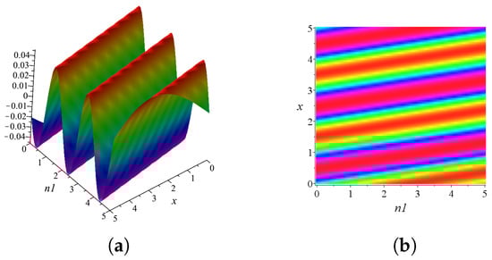
Figure 1. A one-periodic wave of Equation (3). This figure can be regarded as a superposition of a series of soliton waves. (a) Three-dimensional stereogram of one-periodic wave when $n_2=1$. (b) Density plot of the one-periodic wave solution.

3.2. Asymptotic Properties of the One-Periodic Wave Solution

Next, we consider the asymptotic properties of the one-periodic wave solution and establish the relationship of soliton solutions and periodic solutions by taking a limit condition. For this purpose, we give the expansions of the matrix $A={\left(a_{ij}\right)}_{2\times 2}$, the vectors ${(d_1,d_2)}^T$ and ${(k,c)}^T$

$$\begin{array}{ccc}& & \left(\begin{array}{cc}{a}_{11}& a_{12}\\ a_{21}& a_{22}\end{array}\right)=A_0+A_1\varphi +A_2{\varphi }^2+\cdots ,\hfill \\ & & \left(\begin{array}{c}{d}_1\\ d_2\end{array}\right)=D_0+D_1\varphi +D_2{\varphi }^2+\cdots ,\hfill \\ & & \left(\begin{array}{c}k\\ c\end{array}\right)=X_0+X_1\varphi +X_2{\varphi }^2+\cdots ,\hfill \end{array}$$

According to the expression of $a_{ij}$, $d_j$ ($i,j=1,2$) in (21) and expanding these elements to be the sum of $\varphi$, we have

$$\begin{array}{ccc}& & A_0=\left(\begin{array}{cc}0& 1\\ 0& 0\end{array}\right),A_1=\left(\begin{array}{cc}0& 0\\ 4a_1{a}_2\pi i\sinh \pi i(l-w)& 2\cosh \pi i(l+w)\end{array}\right),\hfill \\ & & A_2=\left(\begin{array}{cc}8a_1{a}_2\pi i\sinh 2\pi i(l-w)& 2\cosh 2\pi i(l+w)\\ 0& 0\end{array}\right),A_3=A_4=\left(\begin{array}{cc}0& 0\\ 0& 0\end{array}\right),\hfill \\ & & A_5=\left(\begin{array}{cc}0& 0\\ 12a_1{a}_2\pi i\sinh 3\pi i(l-w)& 2\cosh 3\pi i(l+w)\end{array}\right),\cdots \hfill \end{array}$$

$$\begin{array}{ccc}& & D_0=\left(\begin{array}{c}0\\ 0\end{array}\right),D_1=\left(\begin{array}{c}0\\ 2(a_2-a_1)(\cosh \pi i(l-w)-\cosh \pi i(l+w))\end{array}\right),\hfill \\ & & D_2=\left(\begin{array}{c}2(a_2-a_1)(\cosh 2\pi i(l-w)-\cosh 2\pi i(l+w))\\ 0\end{array}\right),D_3=D_4=\left(\begin{array}{c}0\\ 0\end{array}\right),\hfill \\ & & D_5=\left(\begin{array}{c}0\\ 2(a_2-a_1)(\cosh 3\pi i(l-w)-\cosh 3\pi i(l+w))\end{array}\right),\cdots \hfill \end{array}$$

Therefore, we obtain the following result

$$X_0=\left(\begin{array}{c}{k}_0\\ 0\end{array}\right),X_1=\left(\begin{array}{c}0\\ 0\end{array}\right),X_2=\left(\begin{array}{c}{k}_2\\ c_2,\end{array}\right),$$

(24)

where $k_0$ and $c_2$ have the following expressions

$$\begin{array}{cc}\hfill k_0& ={\displaystyle \frac{(a_2-a_1)(\cosh \pi i(l-w)-\cosh \pi i(l+w))}{2a_1{a}_2\pi i\sinh \pi i(l-w)}},\hfill \\ \hfill c_2& =2(a_2-a_1)[\cosh 2\pi i(l-w)-\cosh 2\pi i(l+w)\hfill \\ \hfill & -{\displaystyle \frac{4\left(\cosh \pi i\right(l-w)-\cosh \pi i(l+w\left)\right)\sinh 2\pi i(l-w)}{\sinh \pi i(l-w)}}].\hfill \end{array}$$

(25)

The relation between the periodic wave solution and the one-soliton solution is given by Theorem 1.

Theorem 1.

Assume that the vector ${(k,c)}^T$ is a solution of the system (22). For the one-periodic wave solution in (23), we take

$$k={\displaystyle \frac{r}{2\pi i}},l={\displaystyle \frac{p}{2\pi i}},w={\displaystyle \frac{q}{2\pi i}},{\eta }_0={\displaystyle \frac{{\xi }_0+\pi b}{2\pi i}},$$

(26)

where r, p, q and ${\xi }_0$ are the same as those in expressions (6)–(7). Then, we have the following asymptotic properties

$$c\to 0,\eta \to {\displaystyle \frac{\xi +\pi b}{2\pi i}},\theta (\eta ,b)\to 1+e^{\xi },\xi =rx+p{n}_1+q{n}_2+{\xi }_0,\varphi \to 0.$$

Proof. 

Firstly, by using the formula in (24), parameters k and c are written as

$$k=k_0+k_2{\varphi }^2+\cdots =k_0+o\left(\varphi \right),c=0+c_2{\varphi }^2+\cdots =o\left(\varphi \right),$$

(27)

which implies that $c\to 0$ as $\varphi \to 0$. Now we expand the periodic wave function $\theta (\eta ,b)$ in (12) as the form

$$\begin{array}{cc}\hfill \theta (\eta ,b)& =1+(e^{2\pi i\eta }+e^{-2\pi i\eta })\varphi +(e^{4\pi i\eta }+e^{-4\pi i\eta }){\varphi }^4+(e^{6\pi i\eta }+e^{-6\pi i\eta }){\varphi }^9+\cdots \hfill \\ & =1+e^{{\eta }^{\prime }}+(e^{-{\eta }^{\prime }}+e^{2{\eta }^{\prime }}){\varphi }^2+(e^{-2{\eta }^{\prime }}+e^{3{\eta }^{\prime }}){\varphi }^6+\cdots ,\hfill \end{array}$$

and, accordingly, ${\eta }^{\prime }$ has the following form

$${\eta }^{\prime }=2\pi i\eta -\pi b=2\pi ikx+2\pi il{n}_1+2\pi iw{n}_2+2\pi i{\eta }_0-\pi b=rx+p{n}_1+q{n}_2+{\xi }_0.$$

According to the expression of k in (27), we have

$${\eta }^{\prime }\to k_{0}x+p{n}_1+q{n}_2+{\xi }_0,\varphi \to 0,$$

where the expression of $k_0$ in (25) is consistent with the expression of r in the dispersion relation (6). Thus we obtain

$$\theta (\eta ,b)\to 1+{\mathrm{e}}^{\xi },\varphi \to 0.$$

which shows that one periodic wave solution tends to the one soliton solution (7) under the condition $\varphi \to 0$. □

4. Two-Periodic Wave Solution of the sdKP Equation and Its Asymptotic Property

In this section, the two-periodic wave solution is considered. In the case $N=2$, the Riemann theta function is defined as the following series

$$\theta (\eta ,B)=\theta ({\eta }_1,{\eta }_2,B)=\sum _{s=-\infty }^{+\infty }{\mathrm{e}}^{2\pi i<\eta ,s>-\pi <Bs,s>},$$

(28)

where $s={(s_1,s_2)}^T\in Z^2$, $\eta ={({\eta }_1,{\eta }_2)}^T\in C^2$, ${\eta }_j=k_{j}x+l_j{n}_1+w_j{n}_2+{\eta }_{0j},j=1,2$, the symbols $<,>$ denote the inner product of vectors, and B is a positive-definite and real-valued symmetric matrix, which can take the form

$$B=\left(\begin{array}{cc}{b}_{11}& b_{12}\\ b_{21}& b_{22}\end{array}\right),b_{11}>0,b_{22}>0,b_{11}{b}_{22}-b_{12}{b}_{21}>0.$$

4.1. Two-Periodic Wave Solution

In order to obtain the two-periodic solution, the theta function is substituted into the LHS of Equation (14) and the following result is derived

$$\begin{array}{cc}\hfill & F\theta (\eta ,B)·\theta (\eta ,B)=\sum _{s=-\infty }^{+\infty }\sum _{s^{\prime }=-\infty }^{+\infty }{\mathrm{e}}^{2\pi i<\eta ,s^{\prime }>-\pi <Bs,s^{\prime }>}\hfill \\ \hfill & =\sum _{s=-\infty }^{+\infty }\sum _{s^{\prime }=-\infty }^{+\infty }[a_1{a}_{2}2\pi i<s-s^{\prime },k>\sinh \pi i<s-s^{\prime },l-w>\hfill \\ \hfill & +(a_1-a_2)\cosh \pi i<s-s^{\prime },l-w>+(c+a_2-a_1)\cosh \pi i<s-s^{\prime },l+w>]\hfill \\ \hfill & \times {\mathrm{e}}^{2\pi i<\eta ,s+s^{\prime }>-\pi <BS,s>-\pi <B{s}^{\prime },s^{\prime }>}\hfill \\ \hfill & \stackrel{s^{\prime }=m-s}{=}\sum _{m=-\infty }^{+\infty }\sum _{s=-\infty }^{+\infty }[a_1{a}_{2}2\pi i<2s-m,k>\sinh \pi i<2s-m,l-w>\hfill \\ \hfill & +(a_1-a_2)\cosh \pi i<2s-m,l-w>\hfill \\ \hfill & +(c+a_2-a_1)\cosh \pi i<2s-m,l+w>]{\mathrm{e}}^{2\pi i<\eta ,m>-\pi <BS,s>-\pi <B(m-s),(m-s)>}\hfill \\ \hfill & =\sum _{m=-\infty }^{+\infty }\overline{F}(m_1,m_2)\times {\mathrm{e}}^{2\pi i<\eta ,m>}\hfill \end{array}$$

(29)

where $s^{\prime }={(s_1^{\prime },s_2^{\prime })}^T$, $k={(k_1,k_2)}^T$, $l={(l_1,l_2)}^T$, $w={(w_1,w_2)}^T$. In the above formula, the notation $\overline{F}(m_1,m_2)$ is defined by

$$\begin{array}{cc}\hfill \overline{F}(m_1,m_2)& =\sum _{s=-\infty }^{+\infty }[a_1{a}_{2}2\pi i<2s-m,k>\sinh \pi i<2s-m,l-w>\hfill \\ \hfill & +(a_1-a_2)\cosh \pi i<2s-m,l-w>\hfill \\ \hfill & +(c+a_2-a_1)\cosh \pi i<2s-m,l+w>]\hfill \\ \hfill & \times {\mathrm{e}}^{-\pi <Bs,s>-\pi <B(m-s),(m-s)>}.\hfill \end{array}$$

(30)

Letting the summation index $s_j=s_j^{\prime }+{\delta }_{jl}$ where ${\delta }_{jl}$ is the Kronecker delta, Formula (30) then has the form

$$\begin{array}{cc}\hfill \overline{F}(m_1,m_2)& =\sum _{s=-\infty }^{+\infty }F(2\pi i(\sum _{j=1}^2(2s_j^{\prime }-(m_j-2{\delta }_{jl})))\sinh (\pi i\sum _{j=1}^2(2s_j^{\prime }-(m_j-2{\delta }_{jl}))),\hfill \\ \hfill & \cosh (\pi i\sum _{j=1}^2(2s_j^{\prime }-(m_j-2{\delta }_{jl}))(l_j-w_j)),\cosh (\pi i\sum _{j=1}^2(2s_j^{\prime }-(m_j-2{\delta }_{jl}))(l_j+w_j)),c)\hfill \\ \hfill & \times {\mathrm{e}}^{-\pi <Bs,s>-\pi <B(m-s),(m-s)>}.\hfill \\ \hfill & =\left\{\begin{array}{cc}\overline{F}(m_1-2,m_2){\mathrm{e}}^{-\pi [2(b_{11}{m}_1+b_{12}{m}_2)-2b_{11}]},\hfill & l=1\hfill \\ \overline{F}(m_1,m_2-2){\mathrm{e}}^{-\pi [2(b_{12}{m}_1+b_{22}{m}_2)-2b_{22}]},\hfill & l=2\hfill \end{array}.\right.\hfill \end{array}$$

The above result indicates that $\overline{F}(m_1,m_2),(m_1,m_2)\in Z^2$ is entirely determined by $\overline{F}(0,0)$, $\overline{F}(0,1)$, $\overline{F}(1,0)$ and $\overline{F}(1,1)$. Hence, if the following four equations are satisfied

$$\overline{F}(0,0)=\overline{F}(0,1)=\overline{F}(1,0)=\overline{F}(1,1)=0,$$

(31)

then $\overline{F}(m_1,m_2)=0,(m_1,m_2)\in Z^2,$ so $F\theta (\eta ,B)·\theta (\eta ,B)=0$. That is, $\theta (\eta ,B)$ is an exact solution of Equation (14). Next, by adopting the following notation

$$M=(a_{j1},a_{j2},a_{j3}),j=1,2,3,4,d={(d_1,d_2,d_3,d_4)}^T$$

$$\begin{array}{cc}& a_{j1}=2\pi i{a}_1{a}_2\sum _{s_1,s_2\in Z^2}(2s_1-r_1^j)\sinh \pi i<2s-r^j,l-w>{ϵ}_j(s_1,s_2)\hfill \\ & a_{j2}=2\pi i{a}_1{a}_2\sum _{s_1,s_2\in Z^2}(2s_2-r_2^j)\sinh \pi i<2s-r^j,l-w>{ϵ}_j(s_1,s_2)\hfill \\ & a_{j3}=\sum _{s_1,s_2\in Z^2}(2s_1-r_1^j)\cosh \pi i<2s-r^j,l-w>{ϵ}_j(s_1,s_2)\hfill \\ & d_j=(a_2-a_1)\sum _{s_1,s_2\in Z^2}[\cosh \pi i<2s-r^j,l-w>-\cosh \pi i<2s-r^j,l+w>]{ϵ}_j(s_1,s_2)\hfill \\ & {\varphi }_1={\mathrm{e}}^{-\pi b_{11}},{\varphi }_2={\mathrm{e}}^{-\pi b_{22}},{\varphi }_3={\mathrm{e}}^{-2\pi b_{12}},\hfill \\ & {ϵ}_j(s_1,s_2)={\varphi }_1^{s_1^2+{(s_1-r_i^j)}^2}{\varphi }_2^{s_2^2+{(s_2-r_2^j)}^2}{\varphi }_3^{s_1{s}_2+(s_1-r_1^j)(s_2-r_2^j)},\hfill \\ & r^1=(0,0),r^2=(0,1)r^3=(1,0)r^4=(1,1),r^j=(r_1^j,r_2^j),j=1,2,3,4,\hfill \end{array}$$

Equation (31) can be written as the following system

$$M{(k_1,k_2,c)}^T=d.$$

(32)

Therefore, we obtain a two-periodic wave solution of Equation (3)

$$u=-{\left(\ln \theta (\eta ,B)\right)}_x,$$

(33)

where the parameters $\theta (\eta ,B)$, $k_1$, $k_2$, c and $b_{12}$ are determined by (28) and (32), while other parameters $l_1$, $l_2$, $w_1$, $w_2$, $b_{11}$ and $b_{22}$ are free, which play an important role in the two-periodic wave solution.

4.2. Asymptotic Properties of the Two-Periodic Wave Solution

In what follows, we further analyze the asymptotic properties of the two-periodic wave solution (33), and establish the relation between the two-periodic wave and the two-soliton solution. In much the same way as in Theorem 1, we first give the expansions of the matrix M and d in (32)

$$\begin{array}{cc}\hfill & M=\left(\begin{array}{ccc}0& 0& 1\\ 0& 0& 0\\ 0& 0& 0\\ 0& 0& 0\end{array}\right)+\left(\begin{array}{ccc}0& 0& 1\\ 0& 0& 0\\ m_{11}& 0& m_{31}\\ 0& 0& 0\end{array}\right){\varphi }_1+\left(\begin{array}{ccc}0& 0& 0\\ 0& m_{12}& m_{32}\\ 0& 0& 0\\ 0& 0& 0\end{array}\right){\varphi }_2\hfill \\ \hfill & +\left(\begin{array}{ccc}{m}_{21}& 0& m_{41}\\ 0& 0& 0\\ 0& 0& 0\\ 0& 0& 0\end{array}\right){\varphi }_1^2+\left(\begin{array}{ccc}0& m_{22}& m_{42}\\ 0& 0& 0\\ 0& 0& 0\\ 0& 0& 0\end{array}\right){\varphi }_2^2\hfill \\ \hfill & +\left(\begin{array}{ccc}0& 0& 0\\ 0& 0& 0\\ 0& 0& 0\\ m_1& m_2& m_3\end{array}\right){\varphi }_1{\varphi }_2+o\left({\varphi }_1^m{\varphi }_2^j\right),m+j\ge 2,\hfill \end{array}$$

(34)

in which

$$\begin{array}{cc}\hfill & m_{1j}=4\pi i{a}_1{a}_2\sinh \pi i(l_j-w_j),m_{2j}=8\pi i{a}_1{a}_2\sinh 2\pi i(l_j-w_j),\hfill \\ \hfill & m_{3j}=2\cosh \pi i(l_j-w_j),m_{4j}=2\cosh 2\pi i(l_j-w_j),j=1,2,\hfill \end{array}$$

$$\begin{array}{cc}\hfill & m_1=4\pi i{a}_1{a}_2[{\varphi }_3\sinh \pi i(l_1-w_1+l_2-w_2)+\sinh \pi i(l_1-w_1-l_2+w_2)],\hfill \\ \hfill & m_2=4\pi i{a}_1{a}_2[{\varphi }_3\sinh \pi i(l_1-w_1+l_2-w_2)+\sinh \pi i(l_2-w_2-l_1+w_1)],\hfill \\ \hfill & m_3=2[{\varphi }_3\cosh \pi i(l_1-w_1+l_2-w_2)+\cosh \pi i(l_1-w_1-l_2+w_2)],\hfill \end{array}$$

and

$$\begin{array}{ccc}& & \begin{array}{cc}& d=\left(\begin{array}{c}0\\ 0\\ 0\\ 0\end{array}\right)+\left(\begin{array}{c}0\\ 0\\ d_1\\ 0\end{array}\right){\varphi }_1+\left(\begin{array}{c}0\\ d_2\\ 0\\ 0\end{array}\right){\varphi }_2\hfill \\ & +\left(\begin{array}{c}{d}_3\\ 0\\ 0\\ 0\end{array}\right){\varphi }_1^2+\left(\begin{array}{c}{d}_4\\ 0\\ 0\\ 0\end{array}\right){\varphi }_2^2+\left(\begin{array}{c}0\\ 0\\ 0\\ d_5\end{array}\right){\varphi }_1{\varphi }_2+o\left({\varphi }_1^m{\varphi }_2^j\right),\hfill \end{array}\hfill \\ & & \begin{array}{cc}& d_1=2(a_2-a_1)[\cosh \pi i(l_1-w_1)-\cosh \pi i(l_1+w_1)],\hfill \\ & d_2=2(a_2-a_1)[\cosh \pi i(l_2-w_2)-\cosh \pi i(l_2+w_2)],\hfill \\ & d_3=2(a_2-a_1)[\cosh 2\pi i(l_1-w_1)-\cosh 2\pi i(l_1+w_1)],\hfill \\ & d_4=2(a_2-a_1)[\cosh 2\pi i(l_2-w_2)-\cosh 2\pi i(l_2+w_2)],\hfill \\ & d_5=2(a_2-a_1)[{\varphi }_3\cosh \pi i(l_1-w_1+l_2-w_2)+\cosh \pi i(l_1-w_1-l_2+w_2)\hfill \\ & -{\varphi }_3\cosh \pi i(l_1+w_1+l_2+w_2)-\cosh \pi i(l_1+w_1-l_2-w_2)].\hfill \end{array}\hfill \end{array}$$

(35)

We assume that the solution of system (32) has the following form

$$\begin{array}{cc}\hfill \left(\begin{array}{c}{k}_1\\ k_2\\ c\end{array}\right)& =\left(\begin{array}{c}{k}_{10}\\ k_{20}\\ c_0\end{array}\right)+\left(\begin{array}{c}{k}_{11}\\ k_{21}\\ c_1\end{array}\right){\varphi }_1+\left(\begin{array}{c}{k}_{12}\\ k_{22}\\ c_2\end{array}\right){\varphi }_2+\left(\begin{array}{c}{k}_{13}\\ k_{23}\\ c_3\end{array}\right){\varphi }_1^2+\left(\begin{array}{c}{k}_{14}\\ k_{24}\\ c_4\end{array}\right){\varphi }_2^2\hfill \\ \hfill & +\left(\begin{array}{c}{k}_{15}\\ k_{25}\\ c_5\end{array}\right){\varphi }_1{\varphi }_2+o\left({\varphi }^m{\varphi }^j\right),m+j\ge 2,\hfill \end{array}$$

(36)

then the relation of the two-periodic wave solution and the two-soliton solution is given as follows.

Theorem 2.

If the two-periodic wave solution in the formula (33) satisfies the following condition

$$k_j={\displaystyle \frac{r_j}{2\pi i}},l_j={\displaystyle \frac{p_j}{2\pi i}},w_j={\displaystyle \frac{q_j}{2\pi i}},{\eta }_{0j}={\displaystyle \frac{{\xi }_{0j}+\pi b_{jj}}{2\pi i}},j=1,2,$$

(37)

where $r_j$, $p_j$, $q_j$ and ${\xi }_{0j}$ are the same as those in the two-soliton solution (9), we have the following asymptotic properties

$$c\to 0,{\eta }_j\to {\displaystyle \frac{{\xi }_j+\pi b_{jj}}{2\pi i}},\theta ({\eta }_1,{\eta }_2,B)\to 1+e^{{\xi }_1}+e^{{\xi }_2}+A_{12}{e}^{{\xi }_1+\xi 2},{\varphi }_1,{\varphi }_2\to 0,$$

where $A_{12}=e^{-2\pi b_{12}}$.

Proof. 

Substituting formulae (34)–(36) into the system (32), we get the following equalities

$$\begin{array}{cc}& k_j=k_{j0}+o\left({\varphi }_i{\varphi }_2\right),j=1,2,c=c_3{\varphi }_1^2+c_3{\varphi }_2^2+o\left({\varphi }_1^2{\varphi }_2^2\right),\hfill \\ & {\mathrm{e}}^{-2\pi b_{12}}={\displaystyle \frac{4\pi i{a}_1{a}_2(k_{20}-k_{10})\sinh \pi i({\widehat{l}}_1-{\widehat{l}}_2)+2(a_2-a_1)(\cosh \pi i({\widehat{l}}_1-{\widehat{l}}_2)-\cosh \pi i({\widehat{w}}_1-{\widehat{w}}_2)}{4\pi i{a}_1{a}_2(k_{20}+k_{10})\sinh \pi i({\widehat{l}}_1+{\widehat{l}}_2)+2(a_2-a_1)(\cosh \pi i({\widehat{l}}_1+{\widehat{l}}_2)-\cosh \pi i({\widehat{w}}_1+{\widehat{w}}_2))}},\hfill \end{array}$$

where

$$\begin{array}{cc}& k_{j0}={\displaystyle \frac{(a_2-a_1)(\cosh \pi i{\widehat{l}}_j-\cosh \pi i{\widehat{w}}_j)}{2a_1{a}_2\pi i\sinh \pi i{\widehat{l}}_j}},c_3={\displaystyle \frac{\sinh \pi i{\widehat{l}}_1}{2\sinh 2\pi i{\widehat{l}}_1}},c_4={\displaystyle \frac{\sinh \pi i{\widehat{l}}_2}{2\sinh 2\pi i{\widehat{l}}_2}},\hfill \end{array}$$

and ${\widehat{l}}_j=l_j-w_j$, ${\widehat{w}}_j=l_j+w_j$, then we have $c\to 0$ as ${\varphi }_1,{\varphi }_2\to 0$. As in Theorem 1, we expand the theta function $\theta ({\eta }_1,{\eta }_2,B)$ in (28) as the form

$$\begin{array}{cc}\hfill \theta ({\eta }_1,{\eta }_2,B)& =1+({\mathrm{e}}^{2\pi i{\eta }_1}+{\mathrm{e}}^{-2\pi i{\eta }_1}){\varphi }_1+({\mathrm{e}}^{2\pi i{\eta }_2}+{\mathrm{e}}^{-2\pi i{\eta }_2}){\varphi }_2+\cdots \hfill \\ & +({\mathrm{e}}^{2\pi i({\eta }_1+{\eta }_2)}+{\mathrm{e}}^{-2\pi i({\eta }_1+{\eta }_2)}){\mathrm{e}}^{-2\pi b_{12}}{\varphi }_1{\varphi }_2+\cdots \hfill \\ & =1+{\mathrm{e}}^{{\widehat{\eta }}_1}+{\mathrm{e}}^{{\widehat{\eta }}_2}+{\mathrm{e}}^{{\widehat{\eta }}_1+{\widehat{\eta }}_2-2\pi b_{12}}+{\mathrm{e}}^{-{\widehat{\eta }}_1}{\varphi }_1^2+{\mathrm{e}}^{-{\widehat{\eta }}_2}{\varphi }_2^2+{\mathrm{e}}^{-{\widehat{\eta }}_1-{\widehat{\eta }}_2-2\pi b_{12}}{\varphi }_1^2{\varphi }_2^2+\cdots ,\hfill \end{array}$$

in which ${\widehat{\eta }}_j=2\pi i{\eta }_j-\pi b_{jj},j=1,2$. In this case,

$${\widehat{\eta }}_j=2\pi i{k}_{j}x+2\pi i{l}_j{n}_1+2\pi i{w}_j{n}_2+2\pi i{\eta }_{0j}-\pi b_{jj}=r_{j}x+p_j{n}_1+q_j{n}_2+{\xi }_{0j}.$$

According to expressions of $k_{j0}$ and ${\varphi }_3$ as mentioned above, we obtain

$${\widehat{\eta }}_j\to {\xi }_j,\theta ({\eta }_1,{\eta }_2,B)\to 1+{\mathrm{e}}^{{\xi }_1}+{\mathrm{e}}^{{\xi }_2}+A_{12}{\mathrm{e}}^{{\xi }_1+{\xi }_2},{\varphi }_1,{\varphi }_2\to 0,\mathrm{where}{A}_{12}=e^{-2\pi b_{12}}.$$

Therefore, the two-periodic solution tends to a two-soliton solution of Equation (3) as ${\varphi }_1,{\varphi }_2\to 0$. □

5. Conclusions and Discussion

In this paper, we have studied the semi-discrete KP (sdKP) Equation (3) and established its integrability by constructing a bilinear Bäcklund transformation, a Lax pair, and a nonlinear superposition formula. Using Hirota’s bilinear method, we derived exact periodic solutions in terms of Riemann theta functions. Explicit expressions for one- and two-periodic wave solutions (23) and (33) were obtained by solving the associated dispersion relations and modular constraints. By taking a long-wave limit, we rigorously analyzed the asymptotic behavior of these solutions and showed that, under appropriate scaling, they converge to the classical soliton solutions of the equation. This limiting process not only confirms the consistency of our results with known soliton solutions, but also reveals a deep connection between periodic and localized wave structures in semi-discrete integrable systems.

However, the construction of higher-order periodic wave solutions—such as three-periodic or higher-genus solutions—remains a significant challenge. The number of undetermined parameters increases rapidly, including wave numbers, frequencies, and entries in the Riemann matrix, leading to an overdetermined or incompatible system of nonlinear algebraic equations [20,22]. Moreover, the increasing complexity of the Riemann theta function in higher dimensions poses substantial difficulties for both symbolic computation and asymptotic analysis. As a result, the direct extension of the present method to higher-genus solutions is highly nontrivial and remains an open problem. In Refs. [25,37], the authors solved such overdetermined systems via the Gauss–Newton method, confirming the existence of three-periodic wave solutions in several integrable systems. These results demonstrate that numerical schemes can effectively capture complex quasi-periodic structures in both continuous and discrete settings, suggesting that similar approaches could be applied to the sdKP equation in future work.

On the physical side, the observed formation and control of soliton molecules in ultrafast fiber lasers [38,39] highlight the rich dynamics of coherent structures under parameter tuning. Although direct experimental realization of sdKP solutions remains challenging, qualitative analogies suggest that such discrete integrable models can provide theoretical insights into the design of controllable wave patterns in engineered systems, such as photonic lattices and electrical networks.

References

- Baxter, R.J. Exactly Solved Models in Statistical Mechanics; Academic Press: London, UK, 1982. [Google Scholar]
- Kuniba, A.; Nakanishi, T.; Suzuki, J. T-systems and Y-systems in integrable systems. J. Phys. A Math. Theor. 2011, 44, 103001. [Google Scholar] [CrossRef]
- Ljubotina, M.; Znidaric, M.; Prosen, T. Spin diffusion from an inhomogeneous quench in an integrable system. Nat. Commun. 2017, 8, 16117. [Google Scholar] [CrossRef]
- Doyon, B. Generalized hydrodynamics of the classical Toda system. J. Math. Phys. 2019, 60, 073302. [Google Scholar] [CrossRef]
- Takahashi, D.; Matsukidaira, J. On discrete soliton equations related to cellular automata. Phys. Lett. A 1995, 209, 184–188. [Google Scholar] [CrossRef]
- Nakamura, Y. A new approach to numerical algorithms in terms of integrable systems. In Proceedings of the International Conference on Informatics Research for Development of Knowledge Society Infrastructure, Washington, DC, USA, 1–2 March 2004; Ibaraki, T., Inui, T., Tanaka, K., Eds.; ACM Publication: New York, NY, USA, 2004; pp. 194–205. [Google Scholar]
- Zhang, Y.N.; Tian, L.X. An integrable semi-discretization of the Boussinesq equation. Phys. Lett. A 2016, 380, 3575–3582. [Google Scholar] [CrossRef]
- Suris, Y.B. Discrete time Toda systems. J. Phys. A Math. Theor. 2018, 51, 333001. [Google Scholar] [CrossRef]
- Shinjo, M.; Fukuda, A.; Kondo, K.; Yamamoto, Y.; Ishiwata, E.; Iwasaki, M.; Nakamura, Y. Discrete hungry integrable systems-40 years from the Physica D paper by WW Symes. Phys. D 2022, 439, 133422. [Google Scholar] [CrossRef]
- Doliwa, A. Non-autonomous multidimensional Toda system and multiple interpolation problem. J. Phys. A Math. Theor. 2022, 55, 505202. [Google Scholar] [CrossRef]
- Doliwa, A.; Siemaszko, A. Integrability and geometry of the Wynn recurrence. Numer. Algorithms 2023, 92, 571–596. [Google Scholar] [CrossRef]
- Amjad, Z.; Haider, B.; Ma, W.X. Integrable discretization and multi-soliton solutions of negative order AKNS equation. Qual. Theory Dyn. Syst. 2024, 23 (Suppl. S1), 280. [Google Scholar] [CrossRef]
- Miwa, T. On Hirota’s difference equations. Proc. Jpn. Acad. A Math. Sci. 1982, 58, 9–12. [Google Scholar] [CrossRef]
- Date, E.; Jimbo, M.; Miwa, T. Method for generating discrete solution equations. J. Phys. Soc. Jpn. 1982, 51, 4116–4124. [Google Scholar] [CrossRef]
- Case, K.M. Benjamin-Ono-related equations and their solutions. Proc. Natl. Acad. Sci. USA 1979, 76, 1–3. [Google Scholar] [CrossRef]
- Ablowitz, M.J.; Clarkson, P.A. Solitons, Nonlinear Evolution Equation and Inverse Scattering; Cambridge University Press: Cambridge, UK, 1991. [Google Scholar]
- Hirota, R. The Direct Method in Soliton Theory; Cambridge University Press: Cambridge, UK, 2004. [Google Scholar]
- Li, C.X.; Lafortune, S.; Shen, S.F. A semi-discrete Kadomtsev-Petviashvili equation and its coupled integrable system. J. Math. Phys. 2017, 57, 053503. [Google Scholar] [CrossRef]
- Nakamura, A. A direct method of calculating periodic wave solutions to nonlinear evolution equations. I. exact two-periodic wave solution. J. Phy. Soc. Jpn. 1979, 47, 1701–1705. [Google Scholar] [CrossRef]
- Nakamura, A. A direct method of calculating periodic-wave solutions to nonlinear evolution equations. II. exact I-periodic and 2-periodic wave solutions of the coupled bilinear equations. J. Phys. Soc. Jpn. 1980, 48, 1365–1370. [Google Scholar] [CrossRef]
- Dubrovin, B.A. Theta functions and nonlinear equations. Russ. Math. Surv. 1981, 36, 11. [Google Scholar] [CrossRef]
- Hirota, R.; Masaaki, I. A direct approach to multi-periodic wave solutions to nonlinear evolution equations. J. Phys. Soc. Jpn. 1981, 50, 338–342. [Google Scholar] [CrossRef]
- Fan, E.G. Quasi-periodic waves and an asymptotic property for the asymmetrical Nizhnik-Novikov-Veselov equation. J. Phys. A Math. Theor. 2009, 42, 095206. [Google Scholar] [CrossRef]
- Ma, W.X.; Zhou, R.G.; Gao, L. Exact one-periodic and two-periodic wave solutions to Hirota bilinear equations in (2+1)dimensions. Mod. Phys. Lett. A 2009, 24, 1677–1688. [Google Scholar] [CrossRef]
- Zhang, Y.N.; Hu, X.B.; Sun, J.Q. A numerical study of the 3-periodic wave solutions to KdV-type equations. J. Comp. Phys. 2018, 355, 566–581. [Google Scholar] [CrossRef]
- Fokou, M.; Kofane, T.C.; Mohamadou, A.; Yomba, E. Lump periodic wave, soliton periodic wave, and breather periodic wave solutions for third-order (2+1)-dimensional equation. Phys. Scr. 2021, 96, 055223. [Google Scholar] [CrossRef]
- Yue, J.; Zhao, Z.L. Solitons, breather-wave transitions, quasi-periodic waves abd asymptotic behaviors for a (2+1)-dimensional Boussinesq-type equation. Eur. Phys. J. Plus 2022, 137, 914. [Google Scholar] [CrossRef]
- Geng, X.G.; Zeng, X. Algebro-geometric quasi-periodic solutions to the Satsuma–Hirota hierarchy. Phys. D 2023, 448, 133738. [Google Scholar] [CrossRef]
- Alharbi, M.; Elmandouh, A.; Elbrolosy, M. Study of Soliton Solutions, Bifurcation, Quasi-Periodic, and Chaotic Behaviour in the Fractional Coupled Schrödinger Equation. Mathematics 2025, 13, 3174. [Google Scholar] [CrossRef]
- Zhang, W.G.; Guo, Y.L.; Zhang, X. Periodic wave solutions and solitary wave solutions of Kundu equation. Phys. Scr. 2025, 100, 035217. [Google Scholar] [CrossRef]
- Geng, X.G.; Dai, H.H.; Zhu, J.Y. Decomposition of the discrete Ablowitz-Ladik hierarchy. Stud. Appl. Math. 2007, 118, 281–312. [Google Scholar] [CrossRef]
- Hon, Y.C.; Fan, E.G.; Qin, Z.Y. A kind of explicit quasi-periodic solution and its limit for the Toda lattice equation. Mod. Phys. Lett. B 2008, 22, 547–553. [Google Scholar] [CrossRef]
- Wu, G.C.; Xia, T.C. Uniformly constructing exact discrete soliton solutions and periodic solutions to differential-difference equations. Comput. Math. Appl. 2009, 58, 2351–2354. [Google Scholar]
- Luo, L. Exact periodic wave solutions for the differntial-difference KP equation. Rep. Math. Phys. 2010, 66, 403–417. [Google Scholar]
- Zhao, Q.L.; Li, C.X.; Li, X.Y. Quasi-periodic solutions of a discrete integrable equation with a finite-dimensional integrable symplectic structure. Phys. D 2024, 458, 133992. [Google Scholar] [CrossRef]
- Wan, L.S. Nonlinear Superposition Formula of a Semi-Discrete KP Equation and Its Exact Solutions. Master’s Thesis, Capital Normal University, Beiing, China, 2024. [Google Scholar]
- Zhang, Y.N.; Hu, X.B.; Sun, J.Q. A numerical study of the 3-periodic wave solutions to Toda-type equations. Commun. Comput. Phys. 2019, 26, 579–598. [Google Scholar] [CrossRef]
- Si, Z.Z.; Wang, Y.Y.; Dai, C.Q. Switching, explosion, and chaos of multi-wavelength soliton states in ultrafast fiber lasers. Sci. China-Phys. Mech. Astron. 2024, 67, 274211. [Google Scholar] [CrossRef]
- SI, Z.Z.; Ju, Z.T.; Ren, L.F.; Wang, X.P.; Malomed, B.A.; Dai, C.Q. Polarization-Induced Buildup and Switching Mechanisms for Soliton Molecules Composed of Noise-Like-Pulse Transition States. Laser Photonics Rev. 2025, 19, 2401019. [Google Scholar] [CrossRef]
Disclaimer/Publisher’s Note: The statements, opinions and data contained in all publications are solely those of the individual author(s) and contributor(s) and not of MDPI and/or the editor(s). MDPI and/or the editor(s) disclaim responsibility for any injury to people or property resulting from any ideas, methods, instructions or products referred to in the content. |
© 2025 by the authors. Licensee MDPI, Basel, Switzerland. This article is an open access article distributed under the terms and conditions of the Creative Commons Attribution (CC BY) license (https://creativecommons.org/licenses/by/4.0/).