Consistent Markov Edge Processes and Random Graphs

Abstract

We discuss Markov edge processes $\{Y_e;e\in E\}$ defined on edges of a directed acyclic graph $(V,E)$ with the consistency property ${\mathrm{P}}_{E^{\prime }}(Y_e;e\in E^{\prime })={\mathrm{P}}_E(Y_e;e\in E^{\prime })$ for a large class of subgraphs $(V^{\prime },E^{\prime })$ of $(V,E)$ obtained through a mesh dismantling algorithm. The probability distribution ${\mathrm{P}}_E$ of such edge process is a discrete version of consistent polygonal Markov graphs. The class of Markov edge processes is related to the class of Bayesian networks and may be of interest to causal inference and decision theory. On regular $\nu$-dimensional lattices, consistent Markov edge processes have similar properties to Pickard random fields on ${\mathbb{Z}}^2$, representing a far-reaching extension of the latter class. A particular case of binary consistent edge process on ${\mathbb{Z}}^3$ was disclosed by Arak in a private communication. We prove that the symmetric binary Pickard model generates the Arak model on ${\mathbb{Z}}^2$ as a contour model.

1. Introduction

A Bayesian network is a probabilistic graphical model that represents a set of variables and their conditional dependencies via a directed acyclic graph [Wikipedia]. Bayesian networks are a fundamental concept in learning and artificial intelligence, see [1,2,3]. Formally, a Bayesian network is a random field $X_V=\{X_v;v\in V\}$ indexed by sites $v\in V$ of a directed acyclic graph (DAG) $G=(V,E)$ whose probability distribution writes as a product of conditional probabilities of $X_v$ given its parent variables $X_u,u\in \mathrm{pa}\left(v\right)$, where $\mathrm{pa}\left(v\right)\subset V$ is the set of parents of v.

A Bayesian network is a special case of Markov random field on a (generally undirected) graph $G=(V,E)$. Markov random fields include nearest-neighbor Gibbs random fields and play an important role in many applied sciences including statistical physics and image analysis [4,5,6,7].

As noted in [8,9,10] and elsewhere, manipulating the marginals (e.g., computing the mean or the covariance function) of a Gibbs random field is generally very hard when V is large. A class of Markov random fields on ${\mathbb{Z}}^2$ which avoids this difficulty was proposed by Pickard [10,11] (the main idea of their construction belongs to Verhagen [12], see [11] (p. 718)). Pickard and related unilateral random fields have found useful applications in image analysis, coding, information theory, crystallography and other scientific areas, not least because they allow for efficient simulation procedures [8,9,13,14,15,16].

A Pickard model $X_V$ (rigorously defined in Section 2) is a family of Bayesian networks on rectangular graphs $G=(V,E),V\subset {\mathbb{Z}}^2$ enjoying the important (Kolmogorov) consistency property: for any rectangles $V^{\prime }\subset V$ we have that

$${\mathrm{P}}_{V|V^{\prime }}={\mathrm{P}}_{V^{\prime }},$$

(1)

where ${\mathrm{P}}_V$ is the distribution of $X_V$ and ${\mathrm{P}}_{V|V^{\prime }}$ is the restriction of marginal of $X_V$ on $V^{\prime }\subset V$. Property (1) implies that the Pickard model extends to a stationary random field on ${\mathbb{Z}}^2$ whose marginals coincide with ${\mathrm{P}}_V$ and form Markov chains on each horizontal or vertical line.

Arak et al. [17,18] introduced a class of polygonal Markov graphs and random fields $X_T=\{X_t;t\in T\}$ indexed by continuous argument $t\in {\mathbb{R}}^2$ satisfying a similar consistency property: for any bounded convex domains $T^{\prime }\subset T$, the restriction of $X_T$ to $T^{\prime }$ coincides in distribution with $X_{T^{\prime }}$. The above models allow a Gibbs representation but are constructed via equilibrium evolution of a one-dimensional particle system with random piece-wise constant Markov velocities, with birth, death and branching. Particles move independently and interact only at collisions. Similarity between polygonal and Pickard models was noted in [19]. Several papers [20,21,22] used polygonal graphs in landscape modeling and random tesselation problems.

The present paper discusses an extension of polygonal graphs and the Pickard model, satisfying a consistency property similar to (1) but not directly related to lattices or rectangles. The original idea of the construction (communicated to the author by Taivo Arak in 1992) referred to a particle evolution on the three-dimensional lattice ${\mathbb{Z}}^3$. In this paper, the above Arak model is extended to any dimension and discussed in Section 4 in detail. It is a special case of a Markov edge process $Y_E=\{Y_e;e\in E\}$ with probability distribution ${\mathrm{P}}_E$ introduced in Section 3 and defined on edges (arcs) $e\in E$ of a directed acyclic graph (DAG) $G=(V,E)$ as the product over $v\in V$ of the conditional clique probabilities ${\pi }_v\left(y_{{\mathcal{E}}_{\mathrm{out}}\left(v\right)}\right|y_{{\mathcal{E}}_{\mathrm{in}}\left(v\right)})$, somewhat similarly to a Bayesian network, albeit the conditional probabilities refer to collection $y_{{\mathcal{E}}_{\mathrm{out}}\left(v\right)}=\{y_e;e\in {\mathcal{E}}_{\mathrm{out}}\left(v\right)\}$ of ‘outgoing’ clique variables and not to a single ‘child’ $x_v$ as in a Bayesian network. Markov random fields indexed by edges discussed in the literature [5,6,7] are usually defined on undirected graphs through Gibbs representation and experience a similar difficulty of computing their marginal distributions as Gibbsian site models. On the other hand, ‘directed’ Markov edge processes might be useful in causal analysis where edges of DAG $G=(V,E)$ represent ‘decisions’ and $Y_e$ can be interpreted as the (random) ‘cost’ of ‘decision’ $e\in E$.

The main result of this work is Theorem 2, providing sufficient conditions for consistency

$${\mathrm{P}}_{E|E^{\prime }}={\mathrm{P}}_{E^{\prime }},\forall G^{\prime }\prec G$$

(2)

of a family ${\mathrm{P}}_{E^{\prime }},G^{\prime }=(E^{\prime },V^{\prime })\in \mathcal{S}$ of Markov edge processes defined on DAGs, $G^{\prime }$, with the partial order $G^{\prime }=(V^{\prime },E^{\prime })\prec G^{″}=(V^{″},E^{″})$ given by $V^{\prime }\subset V^{″},E^{\prime }\subset E^{″}.$ The sufficient conditions for (2) are expressed in terms of clique distributions ${\pi }_v,v\in V$ and essentially reduce to the marginal independence of incoming and outgoing clique variables (i.e., collections $y_{{\mathcal{E}}_{\mathrm{in}}\left(v\right)}$ and $y_{{\mathcal{E}}_{\mathrm{out}}\left(v\right)}$), see (33) and (34).

The class $\mathcal{S}$ of DAGs $G^{\prime }$ satisfying (2) is of special interest. In Theorem 2, $\mathcal{S}={\mathcal{S}}_{\mathrm{MDA}}\left(G\right)$ is the class of all sub-DAGs obtained from a given DAG $G=(V,E)$ by a mesh dismantling algorithm (MDA). The above algorithm starts by erasing any edge that leads to a sink $v_{+}\in V$ or comes from a source $v_{-}\in V$, and proceeds in the same way and in an arbitrary order, see Definition 4. The class ${\mathcal{S}}_{\mathrm{MDA}}\left(G\right)$ contains several interesting classes of ‘one-dimensional’ and ‘multi-dimensional’ sub-DAGs $G^{\prime }$ on which the restriction in (2) is identified as a Markov chain or a sequence of independent r.v.s (Corollary 2).

Section 4 discusses consistent Markov edge processes on ‘rectangular’ subgraphs of ${\mathbb{Z}}^{\nu }$ endowed with nearest-neighbor edges directed in the lexicographic order. We discuss properties of such edge processes and present several examples of ‘generic’ (common) clique distributions, with particular attention paid to the binary case (referred to as the Arak model). In dimension $\nu =2$ we provide a detailed description of the Arak model in terms of a particle system moving along the edges of ${\mathbb{Z}}^2$. Finally, Section 5 establishes a relation between the Pickard and Arak models, the latter model identified in Theorem 3 as a contour model of the former model under an additional symmetry assumption.

We expect that the present work can be extended in several directions. Similarly to [8,9] and some other related studies, the discussion is limited to discrete probability distributions, albeit continuous distributions (e.g., Gaussian edge processes) are of interest. A major challenge is the application of Markov edge processes to causal analysis and Bayesian inference, bearing in mind the extensive research in the case of Bayesian networks [1,2]. Consistent Markov edge processes on regular lattices may be of interest to pattern recognition and information theory. Some open problems are mentioned in Remark 7.

2. Bayesian Networks and Pickard Random Fields

Let $G=(V,E)$ be a given DAG. A directed edge from $v_1$ to $v_2,v_1\ne v_2$, is denoted as $e=(v_1\to v_2)\in E$. With any vertex $v\in V$ we can associate three sets of edges

$$\begin{array}{ccc}& & {\mathcal{E}}_{\mathrm{in}}\left(v\right):=\{e=(v^{\prime }\to v)\in E,v^{\prime }\in V\},{\mathcal{E}}_{\mathrm{out}}\left(v\right):=\{e=(v\to v^{\prime })\in E,v^{\prime }\in V\},\hfill \\ & & \mathcal{E}\left(v\right):={\mathcal{E}}_{\mathrm{in}}\left(v\right)\cup {\mathcal{E}}_{\mathrm{out}}\left(v\right)\hfill \end{array}$$

(3)

representing the incoming edges, outgoing edges and all edges incident to v. A vertex $v\in V$ is called a source or a sink if ${\mathcal{E}}_{\mathrm{in}}\left(v\right)=\varnothing$ or ${\mathcal{E}}_{\mathrm{out}}\left(v\right)=\varnothing$, respectively. The partial order (reachability relation) $v_1⪯v_2$ on G means that there is a directed path on this DAG from $v_1$ to $v_2$. We write $v_1\prec v_2$ if $v_1⪯v_2,v_1\ne v_2.$ The above partial order carries over to edges of G, namely, $e_1=(v_1^{\prime }\to v_1)\prec e_2=(v_2^{\prime }\to v_2)\iff v_1⪯v_2^{\prime }.$ Following [2], the set of vertices $\mathrm{pa}\left(v\right):=\{v^{\prime }\prec v:(v^{\prime }\to v)\in E\}\subset V$ is called the parents of v, whereas $\mathcal{F}\left(v\right):=\left\{v\right\}\cup \mathrm{pa}\left(v\right)\subset V$ is called the family of v.

Definition 1.

Let $G=(V,E)$ be a given DAG. We call family distribution at $v\in V$ any discrete probability distribution ${\varphi }_v={\varphi }_v\left(x_{\mathcal{F}\left(v\right)}\right),x_{\mathcal{F}\left(v\right)}=(x_{v^{\prime }};v^{\prime }\in \mathcal{F}\left(v\right))$, that is, a sequence of positive numbers ${\varphi }_v\left(x_{\mathcal{F}\left(v\right)}\right)>0$ summing up to 1:

$$\sum _{x_{\mathcal{F}\left(v\right)}}{\varphi }_v\left(x_{\mathcal{F}\left(v\right)}\right)=1.$$

The set of all family distributions ${\varphi }_v$ at $v\in V$ is denoted by ${\Phi }_v\left(G\right)$.

For $v\in V,{\varphi }_v\in {\Phi }_v\left(G\right)$, the conditional probability of $x_v$ given parent configuration $x_{\mathrm{pa}\left(v\right)}=(x_{v^{\prime }};v^{\prime }\in \mathrm{pa}\left(v\right))$ writes as

$$\begin{array}{ccc}\hfill {\varphi }_v\left(x_v\right|x_{\mathrm{pa}\left(v\right)})& =& {\displaystyle \frac{{\varphi }_v\left(x_{\mathcal{F}\left(v\right)}\right)}{{\varphi }_v\left(x_{\mathrm{pa}\left(v\right)}\right)}}\mathrm{if}{\varphi }_v\left(x_{\mathcal{F}\left(v\right)}\right)>0,\hfill \end{array}$$

(4)

with ${\varphi }_v\left(x_v\right|x_{\mathrm{pa}\left(v\right)}):=0$ if ${\varphi }_v\left(x_{\mathcal{F}\left(v\right)}\right)=0$ and ${\varphi }_v\left(x_v\right|x_{\mathrm{pa}\left(v\right)}):={\varphi }_v\left(x_v\right)$ if $\mathrm{pa}\left(v\right)=\varnothing$.

Definition 2.

Let ${\Phi }_V=\{{\varphi }_v;v\in V\}$ be a set of family distributions on DAG $G=(V,E)$. We call a Bayesian network on G corresponding to ${\Phi }_V$ a random process $X_V=\{X_v;v\in V\}$ indexed by vertices (sites) of G and such that for any configuration $x_V=(x_v;v\in V)$

$${\mathrm{P}}_V\left(x_V\right)=\mathrm{P}(X_v=x_v;v\in V)=\prod _{v\in V}{\varphi }_v\left(x_v\right|x_{\mathrm{pa}\left(v\right)}).$$

(5)

We remark that the terminology ‘family distribution’ is not commonplace, whereas the definition of Bayesian network varies in the literature [1,2,23], being equivalent to (5) under the positivity condition ${\mathrm{P}}_V\left(x_V\right)>0.$ In the simplest case of chain graph $G=(V,E)$, $V=\{0,1,\cdots ,n\},E=\left\{\right(0\to 1),\cdots ,(n-1\to n\left)\right\}$ (Example 2 below), a Bayesian network $X_V$ is a Markov chain with transition probabilities ${\varphi }_v\left(x_v\right|x_{v-1})$; particularly, any non-Markovian site process $X_V,V=\{0,1,\cdots ,n\}$ on the above G is not a Bayesian network. In the general case $G=(V,E)$, the conditional (family) distributions ${\varphi }_v\left(x_v\right|x_{\mathrm{pa}\left(v\right)})$ in (5) are most intuitive and often used instead of ${\varphi }_v\left(x_{\mathcal{F}\left(v\right)}\right)$. A Bayesian network satisfies several Markov conditions [2], particularly, the ordered Markov condition:

$${\mathrm{P}}_V\left(x_v\right|x_{v^{\prime }},v^{\prime }\prec v)={\mathrm{P}}_V\left(x_v\right|x_{\mathrm{pa}\left(v\right)})={\varphi }_v\left(x_v\right|x_{\mathrm{pa}\left(v\right)}),v\in V.$$

The Markov properties of site models on directed (not necessary acyclic) graphs are discussed in Lauritzen et al. [24] and other works.

In the rest of this subsection, $G=(V,E)$ is a directed subgraph of the infinite DAG $({\mathbb{Z}}^2,E_{\nearrow }\left({\mathbb{Z}}^2\right))$ with lexicographic partial order $v^{\prime }=(t^{\prime },s^{\prime })\prec v=(t,s)(t,s,t^{\prime },s^{\prime }\in \mathbb{Z})$

$$v^{\prime }⪯v⟺s^{\prime }\le s,t^{\prime }\le t$$

and edge set

$$E_{\nearrow }\left({\mathbb{Z}}^2\right):=\{(v^{\prime }\to v);v,v^{\prime }\in {\mathbb{Z}}^2,v^{\prime }=v-(0,1),v-(1,0),v-(1,1)\}.$$

(6)

The class of ‘rectangular’ subDAGs $G=(V,E)$ with

$$V=\{v\in {\mathbb{Z}}^2:v_{-}⪯v⪯v_{+}\},E=\{e=(v^{\prime }\to v^{″})\in E_{\nearrow }\left({\mathbb{Z}}^2\right),v^{\prime },v^{″}\in V\}$$

(7)

$(\exists v_{\pm }\in {\mathbb{Z}}^2,v_{-}\prec v_{+})$ will be denoted ${\mathcal{G}}_{\mathrm{rec}}\left({\mathbb{Z}}_{\nearrow }^2\right)$. Given two ‘rectangular’ DAGs $G_i=(V_i,E_i)\in {\mathcal{G}}_{\mathrm{rec}}\left({\mathbb{Z}}_{\nearrow }^2\right),i=1,2$, we write $G_1\prec G_2$ if $V_1\subset V_2$. For the generic family in Figure 1, right, the family distribution is is indexed by the elements of the table

$$\begin{array}{cc}\hfill & \left(\begin{array}{cc}C& D\\ A& B\end{array}\right)\end{array}$$

(8)

and written as the joint distribution $\varphi (A,B,C,D)$ of four r.v.s $A,B,C,D$ with $x_{v-(1,1)}=A$, $x_{v-(1,0)}=B,x_{v-(1,0)}=C,x_v=D$. The marginal distributions of these r.v.s are designated by the corresponding subsets of the table (8), e.g., $\varphi \left(A\right)$ is the distribution of r.v. A. The conditional distributions of these r.v.s are denoted as in (4); viz., $\varphi \left(B\right|A)=\varphi (A,B)/\varphi (A)$ is the conditional distribution of B given a value of A.

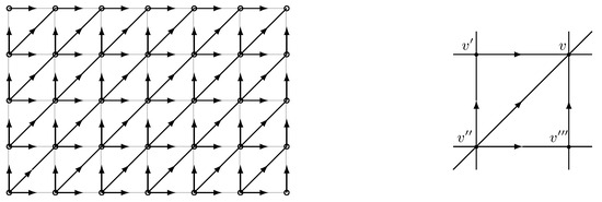
Figure 1. Left: Rectangular DAG in (7); right: generic family $\mathcal{F}\left(v\right)=v\cup \mathrm{pa}\left(v\right),\mathrm{pa}\left(v\right)=\{v^{\prime },v^{″},v^{‴}\}$.

Definition 3.

We call a Pickard model a Bayesian network ${\mathrm{P}}_V$ on DAG $G=(V,E)\in {\mathcal{G}}_{\mathrm{rec}}\left({\mathbb{Z}}_{\nearrow }^2\right)$ with family distribution ${\varphi }_v\equiv \varphi$ independent of $v\in V$ and satisfying the following conditions:

$$\begin{array}{ccc}\hfill & & \varphi \left(A\right)=\varphi \left(B\right)=\varphi \left(C\right)=\varphi \left(D\right),\hfill \\ & & \varphi (A,B)=\varphi (C,D),\varphi (A,C)=\varphi (B,D)\hfill \end{array}$$

(9)

(stationarity) and

$$\begin{array}{c}\hfill \varphi (B,C|A)=\varphi (B\left|A\right)\varphi \left(C\right|A),\varphi (B,C\left|D\right)=\varphi \left(B\right|D\left)\varphi \right(C\left|D\right)\end{array}$$

(10)

(conditional independence).

In a Pickard model, the family $\mathcal{F}\left(v\right)$ of $v\in V$ consists of four points, see Figure 1, except when v belongs to the left lower boundary ${\partial }_{-}V:=\{v=(t,s)\in V:t=t_{-}\mathrm{or}s=s_{-}\},v_{-}=(t_{-},s_{-})$ of rectangle V in (7) and $\left|\mathcal{F}\right(v\left)\right|\le 2$; for $v=v_{-}$ it consists of the single point $\mathcal{F}\left(v_{-}\right)=\left\{v_{-}\right\}$. Accordingly, the family distributions ${\varphi }_v\left(x_{\mathcal{F}\left(v\right)}\right)=\varphi \left(x_{\mathcal{F}\left(v\right)}\right),v\in {\partial }_{-}V$ are marginals of the generic distribution $\varphi$ in Definition 3. We note that Pickard model (also called Pickard random field) is defined in [8,9,10,16] in somewhat different ways, which are equivalent to Definition 3. Let ${\mathcal{V}}_{\mathrm{rec}}\left({\mathbb{Z}}^2\right)$ be the class of all rectangles V in (7).

Theorem 1

([10]). The family $\{{\mathrm{P}}_V;V\in {\mathcal{V}}_{\mathrm{rec}}\left({\mathbb{Z}}^2\right)\}$ of Pickard models on DAGs $G=(V,E)\in {\mathcal{G}}_{\mathrm{rec}}\left({\mathbb{Z}}_{\nearrow }^2\right)$ and corresponding to the same generic family distribution ϕ in (9) and (10) is consistent; in other words, for any $G^{\prime }=(V^{\prime },E^{\prime })\prec G=(V,E),G,G^{\prime }\in {\mathcal{G}}_{\mathrm{rec}}\left({\mathbb{Z}}_{\nearrow }^2\right)$ we have that

$${\mathrm{P}}_{V|V^{\prime }}\left(x_{V^{\prime }}\right)={\mathrm{P}}_{V^{\prime }}\left(x_{V^{\prime }}\right).$$

(11)

Remark 1.

The consistency property in (11) implies that for $G=(V,E)$ in (7), $v_{\pm }=(t_{\pm },s_{\pm })$ and any $s_{-}\le s\le s_{+}$, the restriction of a Pickard model ${\mathrm{P}}_V$ on the horizontal interval $H_s:=\{(t_{-},s),\cdots ,(t_{+},s)\}\subset V$ is a Markov chain

$${\mathrm{P}}_V\left(x_{H_s}\right)=\varphi \left(x_{(t_{-},s)}\right)\varphi \left(x_{(t_{-}+1,s)}\right|x_{(t_{-},s)})\cdots \varphi \left(x_{(t_{+},s)}\right|x_{(t_{+}-1,s)})$$

(12)

with initial distribution $\varphi \left(A\right)$ and transition probabilities $\varphi \left(B\right|A)$. Indeed, $H_s=\{v\in {\mathbb{Z}}^2:(t_{-},s)⪯v⪯(t_{+},s)\}$ is the set of vertices of $G_s\prec G$, and the corresponding ‘one-dimensional’ Pickard model on $G_s$ is defined by (12). In a similar way, the restriction of a Pickard model on a vertical interval $V_t:=\{(t,s_{-}),\cdots ,(t,s_{+})\}\subset V$ is a Markov chain

$${\mathrm{P}}_V\left(x_{V_t}\right)=\varphi \left(x_{(t,s_{-})}\right)\varphi \left(x_{(t,s_{-}+1)}\right|x_{(t,s_{-})})\cdots \varphi \left(x_{(t,s_{+})}\right|x_{(t,s_{+}-1)})$$

(13)

with initial distribution $\varphi \left(A\right)$ and transition probabilities $\varphi \left(C\right|A)$.

Ref. [10] (Thm. 3) extend the Markov chain identifications in (12) and (13) to any non-increasing undirected path in V. This fact and the discussion in Section 3 and Section 5 suggest that the Pickard model and the consistency property in (11) can be extended to non-rectangular index sets $V\subset {\mathbb{Z}}^2$.

Remark 2.

In the binary case $X_v\in \{0,1\}$ or $A,B,C,D\in \{0,1\}$, the distribution ϕ is completely determined by probabilities

$${\varphi }_A:=\mathrm{P}(A=1),\cdots ,{\varphi }_{ABCD}:=\mathrm{P}(A=B=C=D=1).$$

(14)

In terms of (14), conditions (9) and (10) translate to

$$\begin{array}{ccc}\hfill & & {\varphi }_A={\varphi }_B={\varphi }_C={\varphi }_D,{\varphi }_{AB}={\varphi }_{CD},{\varphi }_{AC}={\varphi }_{BD},{\varphi }_{ABC}={\varphi }_{DBC},\hfill \\ & & {\varphi }_{ABC}{\varphi }_A={\varphi }_{AB}{\varphi }_{AC},({\varphi }_A-{\varphi }_{AB})({\varphi }_A-{\varphi }_{AC})=({\varphi }_{BC}-{\varphi }_{ABC})(1-{\varphi }_A),\hfill \end{array}$$

(15)

see [10] (p. 666). The special cases ${\varphi }_A=0,1$, ${\varphi }_A={\varphi }_{AB}$ and ${\varphi }_A={\varphi }_{AC}$ correspond to a degenerated Pickard model, the latter two implying $A=B$ and $A=C$, respectively, and leading to a random field which takes constant values on each horizontal (or vertical) line in ${\mathbb{Z}}^2$. Hence, a binary Pickard model can be parametrized by seven parameters,

$$\begin{array}{c}\hfill {\varphi }_A=:a,{\varphi }_{AB}=:b,{\varphi }_{AC}=:c,{\varphi }_{AD},{\varphi }_{ACD},{\varphi }_{ABD},{\varphi }_{ABCD},\end{array}$$

(16)

as ${\varphi }_{ABC},{\varphi }_{BC}$ in the non-degenerated case can be found from $a,b,c$:

$${\varphi }_{ABC}={\displaystyle \frac{bc}{a}},{\varphi }_{BC}={\displaystyle \frac{bc}{a}}+{\displaystyle \frac{(a-b)(a-c)}{1-a}},a\ne 0,1.$$

(17)

The parameters in (16) satisfy natural constraints resulting from their definition as probabilities, particularly, $1\ge a\ge b\vee c$.

3. Markov Edge Process: General Properties and Consistency

It is convenient to allow G to have isolated vertices, which of course can be removed w.l.g., our interest primarily being focused on edges. The directed line graph $G_E^{\to }=(V\left(G_E^{\to }\right),E\left(G_E^{\to }\right))$ of DAG $G=(V,E)$ is defined as the graph whose set of vertices is $V\left(G_E^{\to }\right):=E$ is the same as that of an undirected line graph, and the set of (directed) edges is

$$E\left(G_E^{\to }\right):=\{(e_1\to e_2):e_1\in {\mathcal{E}}_{\mathrm{in}}\left(v\right),e_2\in {\mathcal{E}}_{\mathrm{out}}\left(v\right)(\exists v\in V)\}$$

Note that $G_E^{\to }$ is acyclic, and hence a DAG.

Given a DAG $G=(V,E)$, we denote as $\mathcal{S}\left(G\right)$ the class of all non-empty sub-DAGs (subgraphs) $G^{\prime }=(V^{\prime },E^{\prime })$ with $V^{\prime }\subset V,E^{\prime }\subset E$.

Definition 4.

A transformation $G{\to }_{+}{G}^{\prime }\in \mathcal{S}\left(G\right)$ is said to be a top mesh dismantling algorithm (top MDA) if it erases an edge $e^{\prime }\in {\mathcal{E}}_{\mathrm{in}}\left(v_{+}\right)$ leading to a sink $v_{+}\in V$; in other words, if $G^{\prime }=(V^{\prime },E^{\prime })$ with

$$\begin{array}{c}\hfill V^{\prime }=V,E^{\prime }=E\setminus \left\{e^{\prime }\right\},e^{\prime }\in {\mathcal{E}}_{\mathrm{in}}\left(v_{+}\right),{\mathcal{E}}_{\mathrm{out}}\left(v_{+}\right)=\varnothing .\end{array}$$

(18)

Similarly, a transformation $G{\to }_{-}{G}^{\prime }\in \mathcal{S}\left(G\right)$ is said to be a bottom mesh dismantling algorithm (bottom MDA) if it erases an edge $e^{\prime }\in {\mathcal{E}}_{\mathrm{out}}\left(v_{-}\right)$ starting from a source $v_{-}\in V$, in other words, if $G^{\prime }=(V^{\prime },E^{\prime })$ with

$$V^{\prime }=V,E^{\prime }=E\setminus \left\{e^{\prime }\right\},e^{\prime }\in {\mathcal{E}}_{\mathrm{out}}\left(v_{-}\right),{\mathcal{E}}_{\mathrm{in}}\left(v_{-}\right)=\varnothing .$$

We denote as ${\mathcal{S}}_{\mathrm{MDA}}^{+}\left(G\right),{\mathcal{S}}_{\mathrm{MDA}}^{-}\left(G\right)$ and ${\mathcal{S}}_{\mathrm{MDA}}\left(G\right)$ the classes of DAGs containing G and the subDAGs $G^{\prime }\in \mathcal{S}\left(G\right)$ which can be obtained from G by succesively applying a top MDA, bottom MDA, or both types of MDA in an arbitrary order:

$$\begin{array}{ccc}\hfill {\mathcal{S}}_{\mathrm{MDA}}^{+}\left(G\right)& :=& \left\{G\right\}\cup \{G^{\prime }=G_k,k\ge 1\},G{\to }_{+}{G}_1{\to }_{+}{G}_2{\to }_{+}\cdots {\to }_{+}{G}_k,\hfill \\ \hfill {\mathcal{S}}_{\mathrm{MDA}}^{-}\left(G\right)& :=& \left\{G\right\}\cup \{G^{\prime }=G_k,k\ge 1\},G{\to }_{-}{G}_1{\to }_{-}{G}_2{\to }_{-}\cdots {\to }_{-}{G}_k,\hfill \\ \hfill {\mathcal{S}}_{\mathrm{MDA}}\left(G\right)& :=& \left\{G\right\}\cup \{G^{\prime }=G_k,k\ge 1\},G{\to }_{\pm }{G}_1{\to }_{\pm }{G}_2{\to }_{\pm }\cdots {\to }_{\pm }{G}_k\hfill \end{array}$$

Note that the above transformations may lead to a subDAG $G^{\prime }$ containing isolated vertices which can be removed from $G^{\prime }$ w.l.g. Figure 2 illustrates that ${\mathcal{S}}_{\mathrm{MDA}}\left(G\right)\ne \mathcal{S}\left(G\right)$ in general.

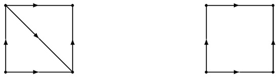
Figure 2. SubDAG $G^{\prime }$ (right) cannot be obtained from DAG G (left) by MDA.

Definition 5.

A subDAG $G^{″}=(V^{″},E^{″})\in \mathcal{S}\left(G\right)$ is said to be the following:

(i) 

An interval DAG if

$$V^{″}=\{v\in V:v_1⪯v⪯v_2\},E^{″}=\{e=(v^{\prime }\to v^{″})\in E:v^{\prime },v^{″}\in V^{″}\}$$

(19)

for some $v_1\prec v_2,v_i\in V,i=1,2$;

(ii) 

A chain DAG if $V^{″}=\{v_1=v_1^{″}\prec v_2^{″}\prec \cdots \prec v_k^{″}=v_2,E^{″}=\{(v_1^{″}\to v_2^{″}),\cdots ,(v_{k-1}^{″}\to v_k^{″})\}(\exists k\ge 1)$, for some $v_1\prec v_2,v_i\in V,i=1,2;$

(iii) 

A source-to-sink DAG if any edge $e=(v^{\prime }\to v^{″})\in E^{″}$ connects a source $v^{\prime }$ of $G^{″}$ to a sink $v^{″}$ of $G^{″}$.

The corresponding classes of subDAGs $G^{″}=(V^{″},E^{″})$ in Definition 5 (i)–(iii) will be denoted by ${\mathcal{S}}_{\mathrm{int}}\left(G\right),{\mathcal{S}}_{\mathrm{chain}}\left(G\right)$ and ${\mathcal{S}}_{\mathrm{sts}}\left(G\right)$.

Proposition 1.

For any DAG $G=(V,E)$ we have that

$${\mathcal{S}}_{\mathrm{int}}\left(G\right)\subset {\mathcal{S}}_{\mathrm{MDA}}\left(G\right).{\mathcal{S}}_{\mathrm{chain}}\left(G\right)\subset {\mathcal{S}}_{\mathrm{MDA}}\left(G\right).{\mathcal{S}}_{\mathrm{sts}}\left(G\right)\subset {\mathcal{S}}_{\mathrm{MDA}}\left(G\right).$$

(20)

Proof. 

The proof of each inclusion in (20) proceeds by induction on the number $\left|E\right|$ of edges of G. Clearly, the proposition holds for $\left|E\right|=1$. Assume it holds for $\left|E\right|=n-1$; we will show that it holds for $\left|E\right|=n.$ The induction step $n-1\to n$ for the three relation in (20) is proved as follows.

(i)

Fix $v_1\prec v_2$ and $G^{″}=(V^{″},E^{″})\in \mathcal{S}\left(G^{\prime }\right)$ to be as in (19). Let $\{v_{+,1},\cdots ,v_{+,m}\}$ be the set of sinks of G. If $v_2$ is a sink and $m=1$ (or $v_2=v_{+,1}$), then $G^{″}=G$ belongs to ${\mathcal{S}}_{\mathrm{MDA}}^{+}\left(G\right)$ by definition of the last class. If $v_2$ is a sink and $m\ge 2$, we can dismantle an edge $e^{\prime }\in {\mathcal{E}}_{\mathrm{in}}\left(v_{+.2}\right)$, and the remaining graph $G^{\prime }=(V^{\prime },E^{\prime })$ in (18) has $n-1$ edges and contains $G^{″}=(V^{″},E^{″})$, meaning the inductive assumption applies, proving $G^{″}\in {\mathcal{S}}_{\mathrm{MDA}}^{+}\left(G^{\prime }\right)\subset {\mathcal{S}}_{\mathrm{MDA}}^{+}\left(G\right)\subset {\mathcal{S}}_{\mathrm{MDA}}\left(G\right)$.

Next, let $v_2\notin \{v_{+,1},\cdots ,v_{+,m}\}$. Then there is a path in G from $v_2$ to at least one of these sinks. If $v_2\prec v_{+}=v_{+,1}$, we apply a top MDA to $v_{+}$ and see that $G^{\prime }$ in (18) has the number of edges $|E^{\prime }|=n-1$ and contains the interval graph $G^{″}$ in (19), so that the inductive assumption applies to $G^{\prime }$ and consequently to G as well, as before, proving the induction step in case (i).

(ii)

Let $G^{″}$ be a chain between $v_1\prec v_2$ and $G^{″}\ne G$, since $G^{″}=G$ belongs to ${\mathcal{S}}_{\mathrm{MDA}}^{+}\left(G\right)$ by definition. Let $\{v_{+,1},\cdots ,v_{+,m}\}$ be the set of sinks of G. If $v_2$ is a sink and $m=1$ then G contains an edge $e=(v\to v_{+,1})$ which does not belong to $G^{″}$. Then, by removing e from G by top MDA we see that $G^{\prime }=(V^{\prime },E^{\prime })$ in (18) contains the chain $G^{″},$ viz., $G^{″}\in \mathcal{S}\left(G^{\prime }\right)$, and therefore $G^{″}\in {\mathcal{S}}_{\mathrm{MDA}}^{+}\left(G^{\prime }\right)$ by the inductive assumption. If $v_2$ is a sink and $m\ge 2$, we remove from G any edge leading to $v_{+,2}$ and arrive at the same conclusion. If $v_2\notin \{v_{+,1},\cdots ,v_{+,m}\}$ is not a sink, we remove any edge leading to a sink and apply the inductive assumption to the remaining graph $G^{\prime }$ having $n-1$ edges. This proves the induction step in case (ii).

(iii)

Let $G^{″}\ne G,G^{″}\in {\mathcal{S}}_{\mathrm{sts}}\left(G\right)$, $V^{″}=V_{-}^{″}\cup V_{+}^{″},$ where $V_{-}^{″}=\{v_{-,1}^{″},\cdots ,v_{-,k}^{″}\}$ and $V_{+}^{″}=\{v_{+,1}^{″},\cdots ,v_{+,\mathcal{\ell }}^{″}\}$ are the sets of sources and sinks of $G^{″}$, respectively. Let $V_{-}$ and $V_{+}$ be the sets of sources and sinks of $G=(V,E)$. If $V=V_{-}\cup V_{+}$, i.e., G is a source-to-sink DAG, we can remove from it an edge $e\in E,e\notin E^{″}$ and the remaining graph $G^{\prime }$ in (18) contains $G^{″}$ and satisfies the inductive assumption. If G is not a source-to-sink DAG, it contains a sink $v_{+}\notin V_{+}^{″}$ or a source $v_{-}\notin V_{-}^{″}.$ In the first case, there is $e^{\prime }=(v^{\prime },v_{+})\in E,e^{\prime }\notin E^{″}$, which can be removed from G, and the remaining graph $G^{\prime }$ contains $G^{″}$ and satisfies the inductive assumption. The second case follows from the first one by DAG reversion. This proves the induction step $n-1\to n$ in case (iii), hence the proposition.

□

An edge process on DAG $G=(V,E)$ is a family $Y_E=\{Y_e;e\in E\}$ of discrete r.v.s indexed by edges of G. It is identified with a (discrete) probability distribution ${\mathrm{P}}_E\left(y_E\right),y_E=(y_e;e\in E).$

Definition 6.

Let $G=(V,E)$ be a given DAG. A clique distribution at $v\in V$ is any discrete probability distribution ${\pi }_v={\pi }_v\left(y_{\mathcal{E}\left(v\right)}\right),y_{\mathcal{E}\left(v\right)}=(y_e;e\in \mathcal{E}\left(v\right))$, that is, a family of positive numbers ${\pi }_v\left(y_{\mathcal{E}\left(v\right)}\right)>0$ summing up to 1:

$$\sum _{y_{\mathcal{E}\left(v\right)}}{\pi }_v\left(y_{\mathcal{E}\left(v\right)}\right)=1.$$

The set of all clique distributions ${\pi }_v$ at $v\in V$ is denoted by ${\Pi }_v\left(G\right)$.

Given ${\pi }_v\in {\Pi }_v\left(G\right)$, the conditional probabilities of out-configuration $y_{{\mathcal{E}}_{\mathrm{out}}\left(v\right)}=(y_e;e\in {\mathcal{E}}_{\mathrm{out}}\left(v\right))$ given in-configuration $y_{{\mathcal{E}}_{\mathrm{in}}\left(v\right)}=(y_e;e\in {\mathcal{E}}_{\mathrm{in}}\left(v\right))$ write as

$${\pi }_v\left(y_{{\mathcal{E}}_{\mathrm{out}}\left(v\right)}\right|y_{{\mathcal{E}}_{\mathrm{in}}\left(v\right)})={\displaystyle \frac{{\pi }_v\left(y_{\mathcal{E}\left(v\right)}\right)}{{\pi }_v(y_{{\mathcal{E}}_{\mathrm{in}}\left(v\right)})}}$$

with $y_{\mathcal{E}\left(v\right)}=(y_e;e\in {\mathcal{E}}_{\mathrm{out}}\left(v\right)\cup {\mathcal{E}}_{\mathrm{in}}\left(v\right))$ and ${\pi }_v\left(y_{{\mathcal{E}}_{\mathrm{out}}\left(v\right)}\right|y_{{\mathcal{E}}_{\mathrm{in}}\left(v\right)}):=1$ for ${\mathcal{E}}_{\mathrm{out}}\left(v\right)=\varnothing ,$ $:={\pi }_v\left({\mathcal{E}}_{\mathrm{out}}\left(v\right)\right)$ for ${\mathcal{E}}_{\mathrm{in}}\left(v\right)=\varnothing$.

Definition 7.

A Markov edge process on a DAG $G=(V,E)$ corresponding to a given family $\{{\pi }_v;v\in V\}$ of clique distributions ${\pi }_v\in {\Pi }_v\left(G\right)$ is a random process $Y_E=\{Y_e;e\in E\}$ indexed by edges of G and such that for any configuration $y_E=(y_e;e\in E)$

$${\mathrm{P}}_E\left(y_E\right)=\mathrm{P}(Y_e=y_e;e\in E):=\prod _{v\in V}{\pi }_v\left(y_{{\mathcal{E}}_{\mathrm{out}}\left(v\right)}\right|y_{{\mathcal{E}}_{\mathrm{in}}\left(v\right)}).$$

(21)

An edge process $Y_E=\{Y_e;e\in E\}$ on a DAG $G=(V,E)$ can be viewed as a site process on the line graph $G_E=(V\left(G_E\right),E\left(G_E\right))$ of $G=(V,E)$, with $V\left(G_E\right):=E,$ $E\left(G_E\right):=\{(e_1\to e_2):e_1\in {\mathcal{E}}_{\mathrm{in}}\left(v\right),e_2\in {\mathcal{E}}_{\mathrm{out}}\left(v\right)(\exists v\in V)\}.$

Corollary 1.

A Markov edge process ${\mathrm{P}}_E$ in (21) is a Bayesian network on the line DAG $G_E=(V\left(G_E\right),E\left(G_E\right))$ if

$${\pi }_v\left(y_{{\mathcal{E}}_{\mathrm{out}}\left(v\right)}\right|y_{{\mathcal{E}}_{\mathrm{in}}\left(v\right)})=\prod _{e\in {\mathcal{E}}_{\mathrm{out}}\left(v\right)}{\pi }_v\left(y_e\right|y_{{\mathcal{E}}_{\mathrm{in}}\left(v\right)}),\forall v\in V.$$

(22)

Condition (22) can be rephrased as the statement that ’outgoing’ variables $Y_e,e\in {\mathcal{E}}_{\mathrm{out}}\left(v\right)$ are conditionally independent given ‘ingoing’ variables $Y_{e^{\prime }},e^{\prime }\in {\mathcal{E}}_{\mathrm{in}}\left(v\right)$ for each node $v\in V$. Analogously, ${\mathrm{P}}_E$ in (21) is a Bayesian network on the reversed line graph $G_E^{\leftarrow }$ under a symmetric condition that ‘ingoing’ variables $Y_{e^{\prime }},e^{\prime }\in {\mathcal{E}}_{\mathrm{in}}\left(v\right)$ are conditionally independent given ‘outgoing’ variables $Y_e,e\in {\mathcal{E}}_{\mathrm{out}}\left(v\right)$, for each node $v\in V$.

Definition 8.

Let $G=(V,E)$ be a DAG and ${\mathcal{S}}^{\prime }\left(G\right)\subset \mathcal{S}\left(G\right)$ be a family of subDAGs of G. A family of edge processes $\{{\mathrm{P}}_{E^{\prime }};G^{\prime }=(V^{\prime },E^{\prime })\in {\mathcal{S}}^{\prime }\left(G\right)\}$ is said consistent if

$${\mathrm{P}}_E\left(y_{E^{\prime }}\right)={\mathrm{P}}_{E^{\prime }}\left(y_{E^{\prime }}\right),\forall G^{\prime }=(V^{\prime },E^{\prime })\in {\mathcal{S}}^{\prime }\left(G\right).$$

(23)

Given edge process ${\mathrm{P}}_E$ in (21), we define its restriction on a subDAG $G^{\prime }\in \mathcal{S}\left(G\right)$ as

$${\mathrm{P}}_{E|E^{\prime }}\left(y_{E^{\prime }}\right):={\mathrm{P}}_E\left(y_{E^{\prime }}\right),y_{E^{\prime }}=(y_e;e\in E^{\prime }).$$

(24)

In general, $P_{E|E^{\prime }}$ is not a Markov edge process on $G^{\prime }$, as shown in the following example.

Example 1.

Let $G=(V,E),V=\{1,2,3\},E=\{e_1=(1\to 2),e_2=(1\to 3),e_3=(2\to 3)\},E^{\prime }=\{e_2,e_3\}.$ Then ${\mathrm{P}}_E(y_{e_1},y_{e_2},y_{e_3})={\pi }_1(y_{e_1},y_{e_2}){\pi }_2\left(y_{e_3}\right|y_{e_1})$ and

$$\begin{array}{ccc}\hfill {\mathrm{P}}_{E|E^{\prime }}(y_{e_2},y_{e_3})& =& \sum _{y_{e_1}}{\pi }_1(y_{e_1},y_{e_2}){\pi }_2\left(y_{e_3}\right|y_{e_1}).\hfill \end{array}$$

(25)

The subDAG $G^{\prime }=(V,E^{\prime })$ is composed of two edges going from different sources 1 and 2 to the same sink 3. By definition, a Markov edge process ${\mathrm{P}}_{E^{\prime }}$ on $G^{\prime }$ corresponds to independent $y_{e_2},y_{e_3}$, viz.,

$$\begin{array}{ccc}\hfill {\mathrm{P}}_{E^{\prime }}(y_{e_2},y_{e_3})& =& {\pi }_1^{\prime }\left(y_{e_2}\right){\pi }_2^{\prime }\left(y_{e_3}\right).\hfill \end{array}$$

(26)

It is easy to see that the two probabilities in (25) and (26) are generally different (however, they are equal if ${\pi }_1(y_{e_1},y_{e_2})={\pi }_1\left(y_{e_1}\right){\pi }_1\left(y_{e_2}\right)$ is a product distribution and ${\pi }_1\left(y_{e_1}\right)={\pi }_2\left(y_{e_1}\right)$, in which case ${\pi }_1^{\prime }\left(y_{e_2}\right)={\pi }_1\left(y_{e_2}\right)$ and ${\pi }_2^{\prime }\left(y_{e_3}\right)={\pi }_2\left(y_{e_3}\right)).$

In Example 1, the restriction ${\mathrm{P}}_{E|E^{\prime }}$ to $E^{\prime }=\{e_1,e_2\}$ is a Markov edge process with ${\mathrm{P}}_{E|E^{\prime }}(y_{e_1},y_{e_2})={\pi }_1(y_{e_1},y_{e_2})$. The following proposition shows that a similar fact holds in a general case for subgraphs $G^{\prime }$ obtained from G by applying a top MDA.

Proposition 2.

Let $P_E$ be a Markov edge process on DAG $G=(V,E)$. Then for any $G^{\prime }=(V^{\prime },E^{\prime })\in {\mathcal{S}}_{\mathrm{MDA}}^{+}\left(G\right)$, the restriction ${\mathrm{P}}_{E|E^{\prime }}$ is a Markov edge process on $G^{\prime }$ with clique distribution ${\pi }_v^{\prime }\in {\Pi }_v\left(G^{\prime }\right),v\in V^{\prime }$ given by

$${\pi }_v^{\prime }\left(y_{{\mathcal{E}}^{\prime }\left(v\right)}\right):={\pi }_v\left(y_{{\mathcal{E}}^{\prime }\left(v\right)}\right),v\in V^{\prime }$$

(27)

which is the restriction of clique distributions ${\pi }_v$ to (sub-clique) ${\mathcal{E}}^{\prime }\left(v\right)=\mathcal{E}\left(v\right)\cap E^{\prime }.$

Proof. 

It suffices to prove the proposition for a one-step top MDA, or $G^{\prime }$ in (18). Let ${\mathcal{E}}_{\mathrm{in}}\left(v_{+}\right):=\{e_1=(v_1\to v_{+}),\cdots ,e_k=(v_k\to v_{+})\}$, $k\ge 2$, $e^{\prime }=e_k$. From the definitions in (21) and (27),

$$\begin{array}{ccc}\hfill {\mathrm{P}}_{E|E^{\prime }}\left(y_{E^{\prime }}\right)& =& \prod _{v\in V\setminus \left\{v_k\right\}}{\pi }_v\left(y_{{\mathcal{E}}_{\mathrm{out}}\left(v\right)}\right|y_{{\mathcal{E}}_{\mathrm{in}}\left(v\right)})\sum _{y_{e_k}}{\pi }_{v_k}\left(y_{{\mathcal{E}}_{\mathrm{out}}\left(v_k\right)}\right|y_{{\mathcal{E}}_{\mathrm{in}}\left(v_k\right)})\hfill \\ & =& \prod _{v\in V\setminus \left\{v_k\right\}}{\pi }_v\left(y_{{\mathcal{E}}_{\mathrm{out}}\left(v\right)}\right|y_{{\mathcal{E}}_{\mathrm{in}}\left(v\right)}){\pi }_{v_k}^{\prime }\left(y_{{\mathcal{E}}_{\mathrm{out}}^{\prime }\left(v_k\right)}\right|y_{{\mathcal{E}}_{\mathrm{in}}\left(v_k\right)})=\prod _{v\in V}{\pi }_v^{\prime }\left(y_{{\mathcal{E}}_{\mathrm{out}}^{\prime }\left(v\right)}\right|y_{{\mathcal{E}}_{\mathrm{in}}^{\prime }\left(v\right)}).\hfill \end{array}$$

□

Example 2

(Markov chain). Let $G=(V,E),V=\{0,1,\cdots ,n\},E=\{e_1=(0\to 1),e_2=(1\to 2),\cdots ,e_n=(n-1\to n)\}$ be a chain from 0 to n. The classes ${\mathcal{S}}_{\mathrm{MDA}}^{+}\left(G\right),{\mathcal{S}}_{\mathrm{MDA}}^{-}\left(G\right)$ and ${\mathcal{S}}_{\mathrm{MDA}}\left(G\right)$ consist respectively of all chains from 0 to $j\in \{1,\cdots ,n\}$, from $i\in \{0,\cdots ,n-1\}$ to n and from i to j ($0\le i<j\le n).$ A Markov edge process on the above graph is a Markov chain $Y_E=\{Y_{e_1},\cdots ,Y_{e_n}\}$ with the probability distribution

$${\mathrm{P}}_E(y_{e_1},y_{e_1},\cdots ,y_{e_n})={\pi }_0\left(y_{e_1}\right){\pi }_1\left(y_{e_2}\right|y_{e_1})\cdots {\pi }_{n-1}\left(y_{e_n}\right|y_{e_{n-1}})$$

where ${\pi }_0$ is a (discrete) univariate and ${\pi }_k,1\le k<n-1$ are bivariate probability distributions; ${\pi }_k\left(y_{e_{k+1}}\right|y_{e_k})={\pi }_k(y_{e_k},y_{e_{k+1}})/{\sum }_y{\pi }_k(y_{e_k},y)$ are conditional or transitional probabilities. It is clear that the restriction ${\mathrm{P}}_{E|E^{\prime }}$ on $E^{\prime }=\{e_1,\cdots ,e_j\}$ is a Markov chain with ${\pi }_0^{\prime }={\pi }_0,{\pi }_k^{\prime }={\pi }_k,1\le k<j$; in other words, it satisfies Proposition 2 and (27). However, the restriction ${\mathrm{P}}_{E|E^{\prime }}$ to $E^{\prime }=\{e_i,\cdots ,e_n\}$ or $G^{\prime }=(V^{\prime },E^{\prime })\in {\mathcal{S}}_{\mathrm{MDA}}^{-}\left(G\right)$ is a Markov chain with the initial distribution

$${\pi }_i^{\prime }\left(y_{e_i}\right)=\sum _{{\tilde{y}}_{e_1},\cdots ,{\tilde{y}}_{e_{i-1}}}{\pi }_0\left({\tilde{y}}_{e_1}\right)\prod _{1\le k<i}{\displaystyle \frac{{\pi }_k({\tilde{y}}_{e_k},{\tilde{y}}_{e_{k+1}})}{{\pi }_k\left({\tilde{y}}_{e_k}\right)}},{\tilde{y}}_{e_i}=y_{e_i}$$

which is generally different from ${\pi }_i\left(y_{e_i}\right)$. We conclude that Proposition 2 ((27) in particular) fails for subDAGs $G^{\prime }$ of G obtained by a bottom MDA. On the other hand, ${\pi }_i^{\prime }={\pi }_i,1\le i<n$ hold for the above $G^{\prime },G$ provided the ${\pi }_k$ values satisfy the additional compatibility condition:

$${\pi }_k\left(y_{e_k}\right)={\pi }_{k-1}\left(y_{e_k}\right),e_k=(k-1\to k),k=1,\cdots ,n-1.$$

Proposition 3.

Let ${\mathrm{P}}_E$ be a Markov edge process on DAG $G=(V,E)$ in (21). Then for any edge $e=(v_1\to v_2)\in E$

$$\begin{array}{ccc}\hfill {\mathrm{P}}_E\left(y_e\right|y_{e^{\prime }},e^{\prime }\ne e,e^{\prime }\in E)& =& {\mathrm{P}}_E\left(y_e\right|y_{e^{\prime }},e^{\prime }\in {\mathcal{E}}_{\mathrm{out}}\left(v_2\right)\cup {\mathcal{E}}_{\mathrm{in}}\left(v_1\right))\hfill \\ & =& {\displaystyle \frac{{\pi }_{v_1}\left(y_{{\mathcal{E}}_{\mathrm{out}}\left(v_1\right)}\right|y_{{\mathcal{E}}_{\mathrm{in}}\left(v_1\right)}){\pi }_{v_2}\left(y_{{\mathcal{E}}_{\mathrm{out}}\left(v_2\right)}\right|y_{{\mathcal{E}}_{\mathrm{in}}\left(v_2\right)})}{{\sum }_{{\tilde{y}}_e}{\pi }_{v_1}\left({\tilde{y}}_{{\mathcal{E}}_{\mathrm{out}}\left(v_1\right)}\right|{\tilde{y}}_{{\mathcal{E}}_{\mathrm{in}}\left(v_1\right)}){\pi }_{v_2}\left({\tilde{y}}_{{\mathcal{E}}_{\mathrm{out}}\left(v_2\right)}\right|{\tilde{y}}_{{\mathcal{E}}_{\mathrm{in}}\left(v_2\right)})}}\hfill \end{array}$$

(28)

and

$$\begin{array}{ccc}\hfill {\mathrm{P}}_E\left(y_e\right|y_{e^{\prime }},e^{\prime }\prec e)& =& {\mathrm{P}}_E\left(y_e\right|y_{e^{\prime }},e^{\prime }\in {\mathcal{E}}_{\mathrm{in}}\left(v_1\right))={\pi }_{v_1}\left(y_e\right|y_{{\mathcal{E}}_{\mathrm{in}}\left(v_1\right)}),\hfill \end{array}$$

(29)

with ${\tilde{y}}_E=({\tilde{y}}_e;e\in E)$ satisfying ${\tilde{y}}_{e^{\prime }}=y_{e^{\prime }},e^{\prime }\ne e$.

Proof. 

Relation (28) follows from

$${\mathrm{P}}_E\left(y_e\right|y_{e^{\prime }},e^{\prime }\ne e,e^{\prime }\in E)={\displaystyle \frac{{\mathrm{P}}_E\left(y_E\right)}{{\sum }_{{\tilde{y}}_e}{\mathrm{P}}_E\left({\tilde{y}}_E\right)}}$$

(30)

and the definition in (21), since the products ${\prod }_{v\ne v_1,v_2}$ cancel in the numerator and the denominator of (30).

Consider (29). We use Propositions 1 and 2, according to which the interval DAGs $G_i=(V_i,E_i),V_i:=\{v\in V:v⪯v_i\},i=1,2$ belong to ${\mathcal{S}}_{\mathrm{MDA}}^{+}\left(G\right)$. The ‘intermediate’ DAG $\tilde{G}=(\tilde{V},\tilde{E})$, constructed from $G_1$ by adding the single edge $e=(v_1\to v_2)$, viz., $\tilde{V}:=V_1\cup \left\{v_2\right\},\tilde{E}:=E_1\cup \left\{e\right\}$, also belongs to ${\mathcal{S}}_{\mathrm{MDA}}^{+}\left(G\right)$ since it can be attained from $G_2$ by dismantling all edges with the exception of $\tilde{E}$. Note that $\left\{e\right\}\cup \{e^{\prime }\in E:\prec e\}=\tilde{E}$. Therefore, by Proposition 2, ${\mathrm{P}}_{E|\tilde{E}}\left(y_{\tilde{E}}\right)={\mathrm{P}}_{\tilde{E}}\left(y_{\tilde{E}}\right)$ where ${\mathrm{P}}_{\tilde{E}}$ is a Markov edge process on $\tilde{G}$ with clique distributions

$${\tilde{\pi }}_v\left(y_{\tilde{\mathcal{E}}\left(v\right)}\right):={\pi }_v\left(y_{\tilde{\mathcal{E}}\left(v\right)}\right),v\in \tilde{V}.$$

(31)

The expression in (29) follows from (31) and (28) with E replaced by $\tilde{E}$ by noting that $v_2$ is a sink in $\tilde{G}$; hence, ${\tilde{\pi }}_{v_2}\left(y_{{\tilde{\mathcal{E}}}_{\mathrm{out}}\left(v_2\right)}\right|y_{{\tilde{\mathcal{E}}}_{\mathrm{in}}\left(v_2\right)})=1$, whereas ${\tilde{\pi }}_{v_1}\left(y_{{\tilde{\mathcal{E}}}_{\mathrm{out}}\left(v_1\right)}\right|y_{{\tilde{\mathcal{E}}}_{\mathrm{in}}\left(v_1\right)})={\pi }_{v_2}\left(y_e\right|y_{{\mathcal{E}}_{\mathrm{in}}\left(v_1\right)})$. □

Remark 3.

Note that $e^{\prime }\in {\mathcal{E}}_{\mathrm{out}}\left(v_2\right)\cup {\mathcal{E}}_{\mathrm{in}}\left(v_1\right)$ in the conditional probability on the r.h.s. of (28) are nearest neighbors of e in the line graph (DAG) $G_E=(V\left(G_E\right),E\left(G_E\right))$

Theorem 2.

Let $G=(V,E)$ be a given DAG and ${\mathrm{P}}_E$ a Markov edge process in (21) with clique distributions ${\pi }_v\in {\Pi }_v,v\in V$ satisfying the compatibility condition

$$\begin{array}{c}\hfill {\pi }_{v_1}\left(y_e\right)={\pi }_{v_2}\left(y_e\right),\forall e=(v_1\to v_2)\in E\end{array}$$

(32)

and two marginal independence conditions:

$${\pi }_v\left(y_{{\mathcal{E}}_{\mathrm{out}}\left(v\right)}\right)=\prod _{e\in {\mathcal{E}}_{\mathrm{out}}\left(v\right)}{\pi }_v\left(y_e\right)$$

(33)

and

$${\pi }_v\left(y_{{\mathcal{E}}_{\mathrm{in}}\left(v\right)}\right)=\prod _{e\in {\mathcal{E}}_{\mathrm{in}}\left(v\right)}{\pi }_v\left(y_e\right).$$

(34)

Then the family of Markov edge process ${\mathrm{P}}_{E^{\prime }},G^{\prime }=(V^{\prime },E^{\prime })\in {\mathcal{S}}_{\mathrm{MDA}}\left(G\right)$ with clique distributions ${\pi }_v^{\prime }\in {\Pi }_v,v\in V^{\prime }$ given in (27) is consistent, viz.,

$${\mathrm{P}}_E{|}_{E^{\prime }}={\mathrm{P}}_{E^{\prime }},\forall G^{\prime }=(V^{\prime },E^{\prime })\in {\mathcal{S}}_{\mathrm{MDA}}\left(G\right).$$

(35)

Remark 4.

(i) 

Conditions (33) and (34) do not imply the mutual independence of the in- and out-clique variables $y_{{\mathcal{E}}_{\mathrm{in}}\left(v\right)}$ and $y_{{\mathcal{E}}_{\mathrm{out}}\left(v\right)}$ under ${\pi }_v$.

(ii) 

Conditions (33) and (34) are automatically satisfied if $\mathrm{card}\left({\mathcal{E}}_{\mathrm{in}}\left(v\right)\right),\mathrm{card}\left({\mathcal{E}}_{\mathrm{out}}\left(v\right)\right)\in \{0,1\}$ (Markov chain).

(iii) 

Conditions (33) and (34) are symmetric with regard to DAG reversion (all directions reversed).

(iv) 

In the binary case ($Y_e=0,1$), the value $Y_e=1$ can be interpreted as the presence of a ‘particle’ and $Y_e=0$ as its absence on edge $e\in E$. ‘Particles’ ‘move’ on a DAG $(V,E)$ in the direction of arrows. ‘Particles’ ‘collide’, ‘annihilate’ or ‘branch’ at nodes $v\in V$, with probabilities determined by clique distribution ${\pi }_v$. See Section 4 for a detailed description of particle evolution for the Arak model on ${\mathbb{Z}}^2$.

Proof of Theorem 2. 

It suffices to prove (35) for a one-step MDA:

$$E{\to }_{-}{E}_{-}^{\prime }=E\setminus \left\{e_{-}^{\prime }\right\}\mathrm{and}E{\to }_{+}{E}_{+}^{\prime }=E\setminus \left\{e_{+}^{\prime }\right\}$$

which remove a single edge $e_{-}^{\prime }=(v_{-}\to v^{\prime })$ coming from a source $v_{-}\in V$ and a single edge $e_{+}^{\prime }=(v^{\prime }\to v_{+})$ going to a sink $v_{+}\in V$, respectively. Moreover, it suffices to consider $E_{-}^{\prime }$ only. The proof for $E_{+}^{\prime }$ follows from Proposition 2 and does not require (32)–(34). (It also follows from $E_{-}^{\prime }$ by DAG reversion.) Then, by the marginal independence of ${\pi }_v,v=v_{-},v^{\prime }$ and ${\pi }_{v_{-}}\left(y_{e^{\prime }}\right)={\pi }_{v^{\prime }}\left(y_{e^{\prime }}\right)$,

$$\begin{array}{ccc}\hfill {\mathrm{P}}_E\left(y_E\right)& =& {\pi }_{v_{-}}\left(y_{e^{\prime }}\right)\left(\prod _{e\in {\mathcal{E}}_{\mathrm{out}}\left(v_{-}\right),e\ne e_{-}^{\prime }}{\pi }_{v_{-}}\left(y_e\right)\right){\displaystyle \frac{{\pi }_{v^{\prime }}\left(y_{{\mathcal{E}}_{\mathrm{in}}\left(v^{\prime }\right)\cup {\mathcal{E}}_{\mathrm{out}}\left(v^{\prime }\right)}\right)}{{\pi }_{v^{\prime }}\left(y_{e^{\prime }}\right){\pi }_{v^{\prime }}\left(y_{{\mathcal{E}}_{\mathrm{in}}\left(v^{\prime }\right)\setminus \left\{e^{\prime }\right\}}\right)}}\prod _{v\in V,v\ne v_{-},v^{\prime }}{\pi }_v\left(y_{{\mathcal{E}}_{\mathrm{out}}\left(v\right)}\right|y_{{\mathcal{E}}_{\mathrm{in}}\left(v\right)})\hfill \\ & =& \left(\prod _{e\in {\mathcal{E}}_{\mathrm{out}}\left(v_{-}\right),e\ne e_{-}^{\prime }}{\pi }_{v_{-}}\left(y_e\right)\right){\displaystyle \frac{{\pi }_{v^{\prime }}\left(y_{{\mathcal{E}}_{\mathrm{in}}\left(v^{\prime }\right)\cup {\mathcal{E}}_{\mathrm{out}}\left(v^{\prime }\right)}\right)}{{\pi }_{v^{\prime }}\left(y_{{\mathcal{E}}_{\mathrm{in}}\left(v^{\prime }\right)\setminus \left\{e^{\prime }\right\}}\right)}}\prod _{v\in V,v\ne v_{-},v^{\prime }}{\pi }_v\left(y_{{\mathcal{E}}_{\mathrm{out}}\left(v\right)}\right|y_{{\mathcal{E}}_{\mathrm{in}}\left(v\right)}).\hfill \end{array}$$

From the definition of ${\pi }_v^{\prime }$ in (27), we have that ${\prod }_{e\in {\mathcal{E}}_{\mathrm{out}}\left(v_{-}\right),e\ne e_{-}^{\prime }}{\pi }_{v_{-}}\left(y_e\right)={\pi }_{v_{-}}^{\prime }\left(y_{{\mathcal{E}}_{\mathrm{out}}^{\prime }\left(v_{-}\right)}\right),{\pi }_{v^{\prime }}\left(y_{{\mathcal{E}}_{\mathrm{in}}\left(v^{\prime }\right)\setminus \left\{e^{\prime }\right\}}\right)={\pi }_{v^{\prime }}^{\prime }\left(y_{{\mathcal{E}}_{\mathrm{in}}^{\prime }\left(v^{\prime }\right)}\right),{\prod }_{v\in V,v\ne v_{-},v^{\prime }}{\pi }_v^{\prime }\left(y_{{\mathcal{E}}_{\mathrm{out}}^{\prime }\left(v\right)}\right|y_{{\mathcal{E}}_{\mathrm{in}}^{\prime }\left(v\right)})$, and therefore

$$\begin{array}{ccc}\hfill {\mathrm{P}}_E\left(y_E\right)& =& {\pi }_{v_{-}}^{\prime }\left(y_{{\mathcal{E}}_{\mathrm{out}}^{\prime }\left(v_{-}\right)}\right){\displaystyle \frac{{\pi }_{v^{\prime }}\left(y_{{\mathcal{E}}_{\mathrm{in}}\left(v^{\prime }\right)\cup {\mathcal{E}}_{\mathrm{out}}\left(v^{\prime }\right)}\right)}{{\pi }_{v^{\prime }}^{\prime }\left(y_{{\mathcal{E}}_{\mathrm{in}}^{\prime }\left(v^{\prime }\right)}\right)}}\prod _{v\in V,v\ne v_{-},v^{\prime }}{\pi }_v^{\prime }\left(y_{{\mathcal{E}}_{\mathrm{out}}^{\prime }\left(v\right)}\right|y_{{\mathcal{E}}_{\mathrm{in}}^{\prime }\left(v\right)}),\hfill \end{array}$$

leading to

$$\begin{array}{ccc}\hfill {\mathrm{P}}_E\left(y_{E^{\prime }}\right)& =& {\pi }_{v_{-}}^{\prime }\left(y_{{\mathcal{E}}_{\mathrm{out}}^{\prime }\left(v_{-}\right)}\right){\displaystyle \frac{{\pi }_{v^{\prime }}^{\prime }\left(y_{{\mathcal{E}}_{\mathrm{in}}^{\prime }\left(v^{\prime }\right)\cup {\mathcal{E}}_{\mathrm{out}}^{\prime }\left(v^{\prime }\right)}\right)}{{\pi }_{v^{\prime }}^{\prime }\left(y_{{\mathcal{E}}_{\mathrm{in}}^{\prime }\left(v^{\prime }\right)}\right)}}\prod _{v\in V,v\ne v_{-},v^{\prime }}{\pi }_v^{\prime }\left(y_{{\mathcal{E}}_{\mathrm{out}}^{\prime }\left(v\right)}\right|y_{{\mathcal{E}}_{\mathrm{in}}^{\prime }\left(v\right)})\hfill \\ & =& \prod _{v\in V}{\pi }_v^{\prime }\left(y_{{\mathcal{E}}_{\mathrm{out}}^{\prime }\left(v\right)}\right|y_{{\mathcal{E}}_{\mathrm{in}}^{\prime }\left(v\right)})\hfill \end{array}$$

and proving (35) for $E=E_{-}^{\prime }$ defined above, or the statement of the theorem for a one-step MDA $E\to E_{-}^{\prime }$. □

Corollary 2.

Let ${\mathrm{P}}_E$ be a Markov edge process on DAG $G=(V,E)$ satisfying the conditions of Theorem 2:

(i) 

The restriction ${\mathrm{P}}_{E|E^{\prime }}$ of ${\mathrm{P}}_E$ on a chain DAG $G^{\prime }=(V^{\prime },E^{\prime })\in {\mathcal{S}}_{\mathrm{chain}}\left(G\right),V^{\prime }=\{v_0,v_1,\cdots ,v_k\}$, $E^{\prime }=\{e_1,\cdots ,e_k\},e_i=(v_{i-1}\to v_i)$ is a Markov chain, viz.,

$${\mathrm{P}}_{E|E^{\prime }}(y_{e_1},\cdots ,y_{e_k})={\pi }_{v_0}^{\prime }\left(y_{e_1}\right){\pi }_{v_1}^{\prime }\left(y_{e_2}\right|y_{e_1})\cdots {\pi }_{v_{k-1}}^{\prime }\left(y_{e_k}\right|y_{e_{k-1}})$$

(36)

where

$$\begin{array}{c}\hfill {\pi }_{v_0}^{\prime }\left(y_{e_1}\right)={\pi }_{v_0}\left(y_{e_1}\right),{\pi }_{v_i}^{\prime }(y_{e_{i-1}},y_{e_i})={\pi }_{v_i}(y_{e_{i-1}},y_{e_i}),i=1,\cdots ,k.\end{array}$$

(ii) 

The restriction ${\mathrm{P}}_{E|E^{\prime }}$ of ${\mathrm{P}}_E$ on a source-to-sink DAG $G^{\prime }=(V^{\prime },E^{\prime })\in {\mathcal{S}}_{\mathrm{sts}}\left(G\right)$ is a sequence of independent r.v.s, viz.,

$${\mathrm{P}}_{E|E^{\prime }}(y_e,e\in E^{\prime })=\prod _{v\in V_{-}^{\prime }}\prod _{e\in {\mathcal{E}}_{\mathrm{out}}^{\prime }\left(v\right)}{\pi }_v^{\prime }\left(y_e\right),$$

(37)

where $V_{-}^{\prime }\subset V^{\prime }$ is the set of sources of $G^{\prime }$ and ${\mathcal{E}}_{\mathrm{out}\left(v\right)}^{\prime }:={\mathcal{E}}_{\mathrm{out}}\left(v\right)\cap E^{\prime }$ is the set of edges coming from a source $v\in V_{-}^{\prime }$ and ending into a sink of $G^{\prime }$, ${\pi }_v^{\prime }\left(y_e\right):={\pi }_v\left(y_e\right),e\in {\mathcal{E}}_{\mathrm{out}}^{\prime }\left(v\right).$

Proof. 

(i)

By Proposition 1, $G^{\prime }$ belongs to ${\mathcal{S}}_{\mathrm{MDA}}\left(G\right)$ so that Theorem 2 applies with ${\pi }_v^{\prime }$ in (27) given by (31), resulting in (36).

(ii)

By Proposition 1, $G^{\prime }$ belongs to ${\mathcal{S}}_{\mathrm{MDA}}\left(G\right)$ so that Theorem 2 applies with ${\pi }_v^{\prime }$ in (27) given by

$${\pi }_v^{\prime }\left(y_{{\mathcal{E}}_{\mathrm{out}}^{\prime }\left(v\right)}\right)={\pi }_v\left(y_{{\mathcal{E}}_{\mathrm{out}}^{\prime }\left(v\right)}\right)=\prod _{e\in {\mathcal{E}}_{\mathrm{out}}^{\prime }\left(v\right)}{\pi }_v\left(y_e\right)=\prod _{e\in {\mathcal{E}}_{\mathrm{out}}^{\prime }\left(v\right)}{\pi }_v^{\prime }\left(y_e\right),v\in V_{-}^{\prime },$$

(the second equality holds by (33)), resulting in (37).

□

Remark 5.

A natural generalization of chain and source-to-sink DAGs is a source–chain–sink DAG $G^{\prime }=(V^{\prime },E^{\prime })\in \mathcal{S}\left(G\right)$ with the property that any sink $v_{+}\in V^{\prime }$ is reachable from a source $v_{-}\in V^{\prime }$ by a single chain (directed path). We conjecture that for a source–chain–sink DAG $G^{\prime }$, the restriction ${\mathrm{P}}_{E|E^{\prime }}$ of ${\mathrm{P}}_E$ in Theorem 2 is a product of independent Markov chains on disjointed directed paths of $G^{\prime }$, in agreement with representations (36) and (37) of Corollary 2.

Gibbsian representation of Markov edge processes. Gibbsian representation is fundamental in the study of Markov random fields [4,6]. Gibbsian representation of Pickard random fields was discussed in [8,9,11,12]. The following Corollary 3 provides Gibbsian representation of the consistent Markov edge process in Theorem 2. Accordingly, the set of vertices of DAG $G=(V,E)$ is written as $V=V_0\cup \partial V$, where the boundary $\partial V:=\{v\in V:{\mathcal{E}}_{\mathrm{in}}\left(v\right)=\varnothing \mathrm{or}{\mathcal{E}}_{\mathrm{out}}\left(v\right)=\varnothing \}$ consists of sinks and sources of G and the interior $V_0:=V\setminus \partial V$ of the remaining sites.

Corollary 3.

Let ${\mathrm{P}}_E$ be a Markov edge process on DAG $G=(V,E)$ satisfying the conditions of Theorem 2 and the positivity condition ${\mathrm{P}}_E\left(y_E\right)>0$. Then

$$\begin{array}{ccc}\hfill {\mathrm{P}}_E\left(y_E\right)& =& exp\left\{\sum _{v\in V_0}{Q}_v\left(y_{\mathcal{E}\left(v\right)}\right)+\sum _{v\in \partial V}{Q}_v^{\partial V}\left(y_{\mathcal{E}\left(v\right)}\right)\right\},\hfill \end{array}$$

(38)

where the inner and boundary potentials $Q_v,Q_v^{\partial V}$ are given by

$$\begin{array}{ccc}\hfill Q_v\left(y_{\mathcal{E}\left(v\right)}\right)& :=& log{\displaystyle \frac{{\pi }_v\left(y_{\mathcal{E}\left(v\right)}\right)}{{\prod }_{e\in \mathcal{E}\left(v\right)}{\pi }_v\left(y_e\right)}},Q_v^{\partial V}\left(y_{\mathcal{E}\left(v\right)}\right):=log\prod _{e\in \mathcal{E}\left(v\right)}{\pi }_v\left(y_e\right).\hfill \end{array}$$

(39)

Formula (38) follows by writing (21) as ${\mathrm{P}}_E\left(y_E\right)=exp\left\{{\sum }_{v\in V}\left(log{\pi }_v\left(y_{\mathcal{E}\left(v\right)}\right)-log{\prod }_{e\in {\mathcal{E}}_{\mathrm{in}}\left(v\right)}{\pi }_v\left(y_e\right)\right)\right\}$ and rearranging terms in the exponent using (32)–(34). Note (38) is invariant with regard to graph reversal (direction of all edges reversed). Formally, the inner potentials $Q_v$ in (39) do not depend on the orientation of G, raising the question of the necessity of conditions (33) and (34) in Theorem 2. An interesting perspective seems to be the study of the Markov evolution $\{Y_E\left(t\right);t\ge 0\}$ of Markov edge processes on DAG $G=(V,E)$ with invariant Gibbs distribution in (38).

4. Consistent Markov Edge Process on ${\mathbb{Z}}^{\nu }$ and Arak Model

Let $({\mathbb{Z}}^{\nu },E\left({\mathbb{Z}}^{\nu }\right))$ be an infinite DAG whose vertices are points of regular lattice ${\mathbb{Z}}^{\nu }$ and whose edges are pairs $e=(v\to v^{\prime }),|v-v^{\prime }|=1,v⪯v^{\prime }$ directed in the lexicographic order $v=(t_1,\cdots ,t_{\nu })⪯v^{\prime }=(t_1^{\prime },\cdots ,t_{\nu }^{\prime })$ if and only if $t_i\le t_i^{\prime },i=1,\cdots ,\nu$. We write $v\prec v^{\prime }$ if $v⪯v^{\prime },v\ne v^{\prime }$. A $\tilde{\nu }$-dimensional hyperplane $(1\le \tilde{\nu }<\nu )$

$$H_{\tilde{\nu }}=\{(t_1,\cdots ,t_{\tilde{\nu }},s_{\tilde{\nu }+1},\cdots ,s_{\nu })\in {\mathbb{Z}}^{\nu }:(t_1,\cdots ,t_{\tilde{\nu }})\in {\mathbb{Z}}^{\tilde{\nu }}\}$$

(40)

can be identified with ${\mathbb{Z}}^{\tilde{\nu }}$ for any fixed $(s_{\tilde{\nu }+1},\cdots ,s_{\nu })\in {\mathbb{Z}}^{\nu -\tilde{\nu }}$.

Let ${\mathcal{G}}_{\mathrm{rec}}\left({\mathbb{Z}}^{\nu }\right)$ denote the class of all finite ‘rectangular’ subgraphs of $({\mathbb{Z}}^{\nu },E\left({\mathbb{Z}}^{\nu }\right))$, viz., $(V,E)\in {\mathcal{G}}_{\mathrm{rec}}\left({\mathbb{Z}}^{\nu }\right)$ if $V=\{v\in {\mathbb{Z}}^{\nu }:v_{-}⪯v⪯v_{+}\}$ for some $v_{-}\prec v_{+}\in {\mathbb{Z}}^{\nu },v_{\pm }\in {\mathbb{Z}}^{\nu },$ and $E=\{e=(v\to v^{\prime })\in E\left({\mathbb{Z}}^{\nu }\right),v,v^{\prime }\in V\}.$ We denote

$${\mathcal{G}}_{\mathrm{rec}}\left(V\right)=\{G_{\tilde{\nu }},1\le \tilde{\nu }<\nu \}$$

(41)

the class of all subgraphs $G_{\tilde{\nu }}=(V_{\tilde{\nu }},E_{\tilde{\nu }})$ of $(V,E)\in {\mathcal{G}}_{\mathrm{rec}}\left({\mathbb{Z}}^{\nu }\right)$ formed by intersection $V_{\tilde{\nu }}=V\cap H_{\tilde{\nu }},E_{\tilde{\nu }}=\{e=(v\to v^{\prime })\in E,v,v^{\prime }\in V_{\tilde{\nu }}\}$ with a $\tilde{\nu }$-dimensional hyperplane $H_{\tilde{\nu }}\subset {\mathbb{Z}}^{\nu },H_{\tilde{\nu }}\cap V\ne \varnothing$ that can be identified with an element of ${\mathcal{G}}_{\mathrm{rec}}\left({\mathbb{Z}}^{\tilde{\nu }}\right)$. Particularly, for $\nu =3$ and any $(s_2,s_3)\in {\mathbb{Z}}^2$,

$$H_1=\{(t_1,s_2,s_3):t_1\in \mathbb{Z}\},H_1\cap V\ne \varnothing$$

(42)

and the subgraph $G_1=(V_1,E_1)$ can be identified with a chain

$$\begin{array}{c}\hfill E_1=\{v_1^{-}\to v_1^{-}+1\to \cdots \to v_1^{+}-1\to v_1^{+}\},v_1^{+}>v_1^{-}\end{array}$$

(43)

of length $n=v_1^{+}>v_1^{-}\ge 1$. Similarly, for any $s_3\in \mathbb{Z}$,

$$H_2=\{(t_1,t_2,s_3):(t_1,t_2)\in {\mathbb{Z}}^2\},H_2\cap V\ne \varnothing$$

(44)

and the subgraph $G_2=(V_2,E_2)$ of $G=(V,E)\in {\mathcal{G}}_{\mathrm{rec}}\left({\mathbb{Z}}^3\right)$ is a planar ‘rectangular’ graph belonging to ${\mathcal{G}}_{\mathrm{rec}}\left({\mathbb{Z}}^2\right)$. Note that any subgraph $G_{\tilde{\nu }}\in {\mathcal{G}}_{\mathrm{rec}}\left(V\right)$ is an interval subDAG of $G=(V,E)$ in the sense of Definition 5 (i). From Proposition 1 we obtain the following corollary.

Corollary 4.

Let $G=(V,E)\in {\mathcal{G}}_{\mathrm{rec}}\left({\mathbb{Z}}^{\nu }\right)$. Any subgraph $G_{\tilde{\nu }}\in {\mathcal{G}}_{\mathrm{rec}}\left(V\right),1\le \tilde{\nu }<\nu$ can be obtained by applying an MDA to G.

We designate $Y_1,Y_3,\cdots ,Y_{2\nu -1}$ ‘outgoing’ and $Y_2,Y_4,\cdots ,Y_{2\nu }$ ‘incoming’ clique variables (see Figure 3). Let $\pi$ be a generic clique distribution of random vector $(Y_1,Y_2\cdots ,Y_{2\nu -1},Y_{2\nu })$ on incident edges of $v\in {\mathbb{Z}}^{\nu }$. We use the notation ${\pi }_A\left(y_A\right)=\pi (Y_i=y_i,i\in A),y_A=(y_i,i\in A),A\subset A_{\nu }:=\{1,\cdots ,2\nu \},A\ne \varnothing$. $A_{\nu }=A_{\nu }^{\mathrm{out}}\cup A_{\nu }^{\mathrm{in}},$ $A_{\nu }^{\mathrm{out}}:=\{1,3,\cdots ,2\nu -1\},$ $A_{\nu }^{\mathrm{in}}:=\{2,4,\cdots ,2\nu \}.$

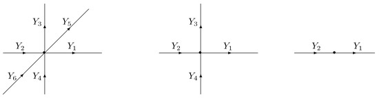
Figure 3. Generic clique variables of Markov edge processes on ${\mathbb{Z}}^{\nu }$, $‘\nu =3,2,1$.

The compatibility and consistency relations in Theorem 2 write as follows for any

$$\begin{array}{c}\hfill {\pi }_i\left(y\right)={\pi }_{i+1}\left(y\right),i=1,3,\cdots ,2\nu -1\end{array}$$

(45)

and

$$\begin{array}{ccc}\hfill {\pi }_{A_{\nu }^{\mathrm{out}}}\left(y_{A_{\nu }^{\mathrm{out}}}\right)& =& \prod _{i\in A_{\nu }^{\mathrm{out}}}{\pi }_i\left(y_i\right),{\pi }_{A_{\nu }^{\mathrm{in}}}\left(y_{A_{\nu }^{\mathrm{in}}}\right)=\prod _{i\in A_{\nu }^{\mathrm{in}}}{\pi }_i\left(y_i\right).\hfill \end{array}$$

(46)

Let ${\Pi }_{\nu }$ be the class of all discrete probability distributions $\pi$ on ${\mathbb{R}}^{2\nu }$ satisfying (45) and (46).

Corollary 5.

Let $Y_E=\{Y_e;e\in E\}$ be a (consistent) Markov edge process on DAG $G=(V,E)\in {\mathcal{G}}_{\mathrm{rec}}\left({\mathbb{Z}}^{\nu }\right)$ with clique distribution $\pi \in {\Pi }_{\nu }$. The restriction

$$Y_{\tilde{E}}:=\{Y_e;e\in \tilde{E}\},\tilde{E}=E\cap H_{\tilde{\nu }}$$

(47)

of $Y_E$ on any $\tilde{\nu }$-dimensional hyperplane $H_{\tilde{\nu }}$ in (40) is a consistent Markov edge process on DAG $G_{\tilde{\nu }}=(\tilde{V},\tilde{E})\in {\mathcal{G}}_{\mathrm{rec}}\left({\mathbb{Z}}^{\tilde{\nu }}\right)$ with generic clique distribution $\tilde{\pi }\left(y_{A_{\tilde{\nu }}}\right):=\pi \left(y_{A_{\tilde{\nu }}}\right),\tilde{\pi }\in {\Pi }_{\tilde{\nu }}$. Particularly, the restriction

$$Y_{E_1}^{\prime }:=\{Y_e;e\in E_1\},E_1=E\cap H_1$$

(48)

of $Y_E$ to a one-dimensional hyperplane $H_1$ in (40) is a reversible Markov chain with the probability distribution

$$\begin{array}{ccc}\hfill \mathrm{P}(Y_{e_1}=y_1,\cdots ,Y_{e_n}=y_n)& =& {\pi }_1^{\prime }\left(y_1\right){\pi }_1^{\prime }\left(y_2\right|y_1)\cdots {\pi }_1^{\prime }\left(y_n\right|y_{n-1}),\hfill \end{array}$$

(49)

where ${\pi }_1^{\prime }(y_1,y_2):={\pi }_{12}(y_1,y_2)$ and ${\pi }_1^{\prime }\left(y_1\right|y_2)={\pi }_1^{\prime }(y_1,y_2)/{\pi }_1^{\prime }\left(y_2\right),{\pi }_1^{\prime }\left(y_2\right)>0$ are the conditional probabilities.

Example 3.

Broken line process. Let $\nu =2$ and $Y_i,i=1,2,3,4$ take integer values $Y_i\in \mathbb{N}=\{0,1,\cdots \}$ and have a joint distribution

$$\begin{array}{ccc}\hfill \pi (y_1,y_2,y_3,y_4)& =& (1-{\lambda }^2){(1-\lambda )}^2{\displaystyle \frac{{\lambda }^{y_1+y_2+y_3+y_4}}{{\lambda }^{|y_3-y_1|}}}\mathbf{1}(y_1-y_3=y_4-y_2),\hfill \end{array}$$

(50)

$y_i\in \mathbb{N},i=1,2,3,4$, where $0<\lambda <1$ is a parameter. Note that for $y_1\ge y_3$

$$\begin{array}{ccc}\hfill \sum _{y_2,y_4\in \mathbb{N}}\pi (y_1,y_2,y_3,y_4)& =& (1-{\lambda }^2){(1-\lambda )}^2{\lambda }^{2y_3}\sum _{y_2,y_4\in \mathbb{N}}{\lambda }^{y_2+y_4}\mathbf{1}(y_1-y_3=y_4-y_2)\hfill \\ & =& {(1-\lambda )}^2{\lambda }^{y_1+y_3}\hfill \end{array}$$

and the last equality is valid for $y_1\le y_3$, too. Therefore, π in (50) is a probability distribution on ${\mathbb{N}}^4$ with (marginals) ${\pi }_{13}$ and ${\pi }_{24}$ written as the product of the geometric distribution with parameter $\lambda >0$. We see that (50) belongs to ${\Pi }_2$ and satisfies (45) and (46) of Corollary 5. The corresponding edge process called the discrete broken line process was studied by Rollo et al. [25] and Sidoravicius et al. [26] in connection with planar Bernoulli first passage percolation. The discrete broken line process can be described as an evolution of particles moving (horizontally or vertically) with constant velocity until collision with another particle and dying upon collision, with independent immigration of pairs of particles. An interesting and challenging open problem is the extension of the broken line process to higher dimensions, particularly to $\nu =3$ or $G\in {\mathcal{G}}_{\mathrm{rec}}\left({\mathbb{Z}}^3\right)$.

Definition 9.

We call an Arak model a binary Markov edge process $Y_E=\{Y_e;e\in E\}$ on a DAG $G=(V,E)\in {\mathcal{G}}_{\mathrm{rec}}\left({\mathbb{Z}}^{\nu }\right)$ with clique distribution $\pi \in {\Pi }_{\nu }$.

We also use the same terminology for the restriction of an Arak model on a subDAG $G^{\prime }\in \mathcal{S}\left(G\right),G\in {\mathcal{G}}_{\mathrm{rec}}\left({\mathbb{Z}}^{\nu }\right)$, and speak about an Arak model on ${\mathbb{Z}}^{\nu }$ since $Y_E$ extends to infinite DAG $({\mathbb{Z}}^{\nu },E\left({\mathbb{Z}}^{\nu }\right))$; the extension $Y=\{Y_e;e\in E\left({\mathbb{Z}}^{\nu }\right)\}$ is a stationary binary random field whose restriction coincides with $Y_E$. Note that when $(Y_1,\cdots ,Y_{2\nu })\in {\{0,1\}}^{2\nu }$, the clique distribution $\pi$ is determined by $2^{2\nu }-1$ probabilities

$$p_A:=\mathrm{P}(Y_i=1,i\in A),A\subset A_{\nu },A\ne \varnothing .$$

(51)

Particularly, for $\nu =3$ the compatibility and consistency relations in (45) and (46) read as

$$\begin{array}{ccc}\hfill & & p_1=p_2,p_3=p_4,p_5=p_6,\hfill \\ & & p_{135}=p_1{p}_3{p}_5,p_{13}=p_1{p}_3,p_{15}=p_1{p}_5,p_{15}=p_1{p}_5,\hfill \\ & & p_{246}=p_2{p}_4{p}_6,p_{24}=p_2{p}_4,p_{26}=p_2{p}_6,p_{46}=p_4{p}_6.\hfill \end{array}$$

(52)

The resulting consistent Markov edge process on ${\mathbb{Z}}^3$ depends on $63-3-8=52$ parameters. In the lattice isotropic case it depends on nine parameters $p_1,p_{13},p_{14},p_{135},p_{123},p_{1234},p_{1345},$$p_{12345},p_{123456}$ satisfying two consistency equations, $p_{135}=p_1^3$ and $p_{13}=p_1^2$, resulting in a seven-parameter isotropic binary edge process communicated to the author by T. Arak.

Denote $v_i:=(\underset{i-1}{\underbrace{0,\cdots ,0}},1,0,\cdots ,0)\in {\mathbb{R}}^{\nu },1\le i\le \nu$ unit vectors in ${\mathbb{Z}}^{\nu }$, $e_i=(v\to v+v_i),$ ${\tau }_n{e}_i:=(v+n{v}_i\to v+(n+1)v_i)$—edges parallel to vectors $v_i,1\le i\le \nu .$ The following corollary is a consequence of Corollary 5 and the formula for the transition probabilities of a binary Markov chain in Feller [27] (Ch.16.2).

Corollary 6.

The covariance function of an Arak model. Let $Y_E$ be an Arak model on DAG $G=(V,E)\in {\mathcal{G}}_{\mathrm{rec}}\left({\mathbb{Z}}^{\nu }\right)$. Then for any $1\le i\le \nu$, $n\in \mathbb{N},e_i\in E,{\tau }_n{e}_i\in E$,

$$\begin{array}{ccc}\hfill \mathrm{E}{Y}_{e_i}{Y}_{{\tau }_n{e}_i}& =& p_{2i}^2+p_{2i}(1-p_{2i}){\left({\displaystyle \frac{p_{2i-1,2i}-p_{2i}^2}{p_{2i}(1-p_{2i})}}\right)}^n,\hfill \end{array}$$

(53)

where $p_{2i}=\mathrm{P}(Y_{e_i}=1)=\mathrm{P}(Y_{2i-1}=1),p_{2i-1,2i}=\mathrm{P}(Y_{e_i}=Y_{{\tau }_1{e}_i}=1)=\mathrm{P}(Y_{2i-1}=Y_{2i}=1)$ are as in (51).

Remark 6.

The conditional probabilities in Corollary 1 (22) for an Arak model can be expressed through $p_A$ in (51). Particularly, an Arak model in dimension $\nu =2$ is a Bayesian network on the line graph of $({\mathbb{Z}}^2,E\left({\mathbb{Z}}^2\right))$ if

$$\begin{array}{c}\hfill p_{12}^2=p_{1234},p_{123}^2=p_1^2{p}_{1234}.\end{array}$$

In the two-dimensional case $\nu =2$, the Arak model on DAG $G=(V,E)\in {\mathcal{G}}_{\mathrm{rec}}\left({\mathbb{Z}}^2\right)$ is determined by the clique distribution $\pi$ of $(Y_1,Y_2,Y_3,Y_4)$ in Figure 3, middle, with probabilities $p_1=\mathrm{P}(Y_1=1),\cdots ,p_{1234}=\mathrm{P}(Y_1=\cdots =Y_4=1)$ satisfying four conditions:

$$\begin{array}{cc}\hfill & p_1=p_2,p_3=p_4,p_{13}=p_1{p}_3,p_{24}=p_2{p}_4.\end{array}$$

(54)

The resulting edge process depends on 11 = (15 − 4) parameters. In the lattice isotropic case, we have five parameters $p_1,p_{12},p_{13},p_{123},p_{1234}$ satisfying a single condition $p_{13}=p_1^2$ and leading to a four-parameter consistent isotropic binary Markov edge process on ${\mathbb{Z}}^2$. Some special cases of parameters in (54) are discussed in Examples 4–6 below.

The evolution of the particle system. Below, we describe the binary edge process $Y_E$ in Remark 2 on DAG $G=(V,E)\in {\mathcal{G}}_{\mathrm{rec}}\left({\mathbb{Z}}^2\right),V=\{(t,s):1\le t\le m,1\le s\le n\}$ in terms of particle system evolution. The description becomes somewhat simpler by embedding G into $\overline{G}=(\overline{V},\overline{E})$, where

$$\overline{V}=V\cup {\partial }_1^{0}V\cup {\partial }_2^{0}V\cup {\partial }_1^{1}V\cup {\partial }_1^{1}V,$$

where ${\partial }_1^{0}V=\{(1,0),\cdots ,(m,0)\},{\partial }_2^{0}V=\{(0,1),\cdots ,(0,n)\},{\partial }_1^{1}V=\{(1,n+1),\cdots ,(m,n+1)\}$ and ${\partial }_2^{1}V=\{(m+1,1),\cdots ,(m+1,n)\}$ are boundary sites (sources or sinks belonging of the extended graph $\overline{G}$), as shown in Figure 4. The edge process $Y_E$ is obtained from $Y_{\overline{E}}=\{{\overline{Y}}_e:e\in \overline{E}\}$ as $Y_E=\{{\overline{Y}}_e:e\in E\}.$

The presence of a particle on edge $e=(v^{\prime }\to v)\in \overline{E}$ (in the sense explained in Section 2) is identified with ${\overline{Y}}_e=1$. A particle moving on a horizontal or vertical edge is termed horizontal or vertical, respectively. The evolution of particles is described by the following rules:

(p0)

Particles enter the boundary edges ${\partial }_1^{0}E=\{(1,0)\to (1,1),\cdots ,(m,0)\to (m,1))\}$ (vertically) and ${\partial }_2^{0}E=\{(0,1)\to (1,1),\cdots ,(0,n)\to (1,n)\}$ (horizontally) independently of each other with respective probabilities $p_3$ and $p_1$.

(p1)

Particles move along directed edges of $\overline{G}$ independently of each other until collision with another moving particle. A vertical particle entering an empty site $v\in V$ will undergoes one of the following transformations.

(i)

Leaves v as a vertical particle with probability $(p_{34}-p_{134}-p_{234}+p_{1234})/p_3(1-p_1)$;

(ii)

Changes the direction at v to horizontal with probability $(p_{14}-p_{124}-p_{134}+p_{1234})/p_3(1-p_1);$

(iii)

Branches at v into two particles moving into different directions, with probability $(p_{134}-p_{1234})/p_3(1-p_1)$;

(iv)

Dies at v, with probability $(p_4-p_{14}-p_{24}-p_{34}+p_{124}+p_{134}+p_{234}-p_{1234})/p_3(1-p_1)$.

Similarly, a horizontal particle entering an empty site $v\in V$ exhibits transformations as in (i)–(iv) with respective probabilities $(p_{12}-p_{123}-p_{124}+p_{1234})/p_1(1-p_3)$, $(p_{23}-p_{123}-p_{234}+p_{1234})/p_1(1-p_3),$ $(p_{123}-p_{1234})/p_1(1-p_3)$ and $(p_2-p_{12}-p_{23}-p_{24}+p_{123}+p_{124}+p_{234}-p_{1234})/p_1(1-p_3)$.

(p2)

Two (horizontal and vertical) particles entering $v\in V$, either

(i)

both die with probability $(p_{24}-p_{124}-p_{234}+p_{1234})/p_1{p}_3;$ or

(ii)

the horizontal one survives and the vertical one dies with probability $(p_{124}-p_{1234})/p_1{p}_3$. or

(iii)

the vertical one survives and the horizontal one dies with probability $(p_{234}-p_{1234})/p_1{p}_3$. or

(iv)

both particles survive with probability $p_{1234}/p_1{p}_3$.

(p3)

At an empty site $v\in V$ (no particle enters v), one of the following events occurs:

(i)

A single horizontal particle is born, with probability $(p_1-p_{12}-p_{13}-p_{14}+p_{123}+p_{124}+p_{134}-p_{1234})/(1-p_1)(1-p_2);$

(ii)

A single vertical particle is born, with probability $(p_3-p_{13}-p_{23}-p_{34}+p_{123}+p_{134}+p_{234}-p_{1234})/(1-p_1)(1-p_2);$

(iii)

No particles are born, with probability $(1-p_1-p_2-p_3-p_4+p_{12}+p_{13}+p_{14}+p_{23}+p_{24}+p_{34}-p_{123}-p_{124}-p_{134}-p_{234}+p_{1234})/(1-p_1)(1-p_3)$;

(iv)

Two (horizontal and vertical particles) are born, with probability $(p_{13}-p_{123}-p_{134}+p_{1234})/(1-p_1)(1-p_3)$.

The above list provides a complete description of the particle transformations and transition probabilities of the edge process in terms of parameters $p_1,\cdots ,p_{1234}.$

Example 4.

$(Y_1,Y_2,Y_3,Y_4)$ are independent r.v.s, $\mathrm{P}(Y_1=1)=\mathrm{P}\left(Y_2\right)=p_1,\mathrm{P}(Y_3=1)=\mathrm{P}(Y_4=1)=p_3,p_{12}=p_1^2,p_{34}=p_3^2,\cdots ,p_{1234}=p_1^2{p}_3^2$. Accordingly, $Y_e,e\in E$ take independent values on edges of a ’rectangular’ graph $G=(V,E)$, with generally different probabilities $p_1$ and $p_3$ for horizontal and vertical edges. In terms of the particle evolution, this means the ‘outgoing’ particles at each site $v\in V$ being independent and independent of the ‘incoming’ ones.

Example 5.

$p_{12}=p_1$, implying $\mathrm{P}(Y_1\ne Y_2)=0$ and $Y_{e_2}=Y_{e_2+{\tau }_n{e}_1}$ for any horizontal shift of $e_2$. The corresponding edge process $Y_E$ in this case takes constant values on each horizontal line of the rectangle V. Similarly, case $p_{34}=p_3$ leads to $Y_E$ taking constant values on each vertical line of V.

Example 6.

$\mathrm{P}(Y_i\ne Y_j.j\ne i,j=1,2,3,4)=0,i=1,2,3,4$, meaning that none of the four binary edge variables can be different from the remaining three. This implies $\mathrm{E}{Y}_1{Y}_2{Y}_3(1-Y_4)=\cdots =\mathrm{E}(1-Y_1)Y_2{Y}_3{Y}_4=\mathrm{E}{Y}_1{Y}_2{Y}_3{Y}_4,$ or

$$\begin{array}{ccc}\hfill & & p_{123}=p_{124}=p_{134}=p_{234}=p_{1234},\hfill \end{array}$$

(55)

and $\mathrm{E}(1-Y_1)(1-Y_2)(1-Y_3)Y_4=\mathrm{E}(1-Y_1)(1-Y_2)(1-Y_4)Y_3=\mathrm{E}(1-Y_1)(1-Y_3)(1-Y_4)Y_2=\mathrm{E}(1-Y_2)(1-Y_3)(1-Y_4)Y_1=0,$ or

$$\begin{array}{ccc}& & p_{14}=p_{23},p_{12}=p_1-p_{13}-p_{14}+2p_{1234},p_{34}=p_3-p_{13}-p_{23}+2p_{1234}.\hfill \end{array}$$

(56)

The resulting four-parameter model is determined by $p_1,p_3,p_{23},p_{1234}$. In the isotropic case we have two parameters $p_1,p_{1234}$ since $p_3=p_1,p_{23}=p_1^2.$ This case does not allow for the death, birth or branching of a single particle; particles move independently until collision with another moving particle, upon which both colliding particles die or cross each other with probabilities defined in (p1)–(p3) above.

5. Contour Edge Process Induced by Pickard Model

Consider a binary site model $X_V=\{X_v;v\in V\}$ on rectangular graph $G=(V,E),$

$$\begin{array}{ccc}\hfill V& =& \{v\in {\mathbb{Z}}^2:v_{-}⪯v⪯v_{+}\},\hfill \\ \hfill E& =& \{(v\to v^{\prime });v,v^{\prime }\in V,v^{\prime }=v+(0,1),v+(1,0),v+(1,1)\}.\hfill \end{array}$$

(57)

Let ${\tilde{\mathbb{Z}}}^2:={\mathbb{Z}}^2+(1/2,1/2)$ be the shifted lattice, ${\tilde{v}}_{-}=v_{-}+(1/2,1/2),{\tilde{v}}_{+}=v_{+}-(1/2,1/2),{\tilde{v}}_{\pm }\in {\tilde{\mathbb{Z}}}^2$ and $\tilde{G}=(\tilde{V},\tilde{E})\in {\mathcal{G}}_{\mathrm{rec}}\left({\mathbb{Z}}^2\right)$ be the rectangular graph with $\tilde{V}=\{\tilde{v}\in {\tilde{\mathbb{Z}}}^2:{\tilde{v}}_{-}⪯\tilde{v}⪯{\tilde{v}}_{+}\},\tilde{E}=\{\tilde{e}=(\tilde{v}\to {\tilde{v}}^{\prime })\in E\left({\tilde{\mathbb{Z}}}^2\right),\tilde{v},{\tilde{v}}^{\prime }\in \tilde{V}\}.$ For any horizontal or vertical edge $e=(v^{\prime }\to v)\in E\subset E\left({\mathbb{Z}}^2\right)$ we designate

$$\tilde{e}\left(e\right)=(\tilde{v}\to {\tilde{v}}^{\prime })\in \tilde{E}$$

the edge of $\tilde{G}$, which ‘perpendicularly crosses e at the middle’ and is defined formally by

$$\begin{array}{ccc}\hfill \tilde{v}& :=& \left\{\begin{array}{cc}v+\left(1/2,-1/2\right),\hfill & v^{\prime }=v+(1,0),\hfill \\ v+\left(-1/2,1/2\right),\hfill & v^{\prime }=v+(0,1),\hfill \end{array}\right.{\tilde{v}}^{\prime }:=\left\{\begin{array}{cc}\tilde{v}+(0,1),\hfill & v^{\prime }=v+(1,0),\hfill \\ \tilde{v}+(1,0),\hfill & v^{\prime }=v+(0,1).\hfill \end{array}\right.\hfill \end{array}$$

(58)

A Boolean function $\beta =\beta (i,j),i,j\in \{0,1\}$ takes two values, 0 or 1. The class of such Boolean functions has $4^2=16$ elements.

Definition 10.

Let ${\beta }_{\uparrow }$ and ${\beta }_{\to }$ be two Boolean functions. A contour edge process induced by a binary site model $X_V$ on $G=(V,E)$ in (57) and corresponding to ${\beta }_{\uparrow },{\beta }_{\to }$ is a binary edge process on $\tilde{G}=(\tilde{V},\tilde{E})$ defined by

$$\begin{array}{c}\hfill Y_{\tilde{e}\left(e\right)}:=\left\{\begin{array}{cc}{\beta }_{\uparrow }(X_v,X_{v^{\prime }})\hfill & \mathrm{if}{v}^{\prime }=v+(1,0),\hfill \\ {\beta }_{\to }(X_v,X_{v^{\prime }})\hfill & \mathrm{if}{v}^{\prime }=v+(0,1),\hfill \end{array}\right.\end{array}$$

(59)

Probably the most natural contour process occurs in the case of Boolean functions

$$\begin{array}{c}\hfill {\beta }_{\uparrow }(i,j)={\beta }_{\to }(i,j):=\mathbf{1}(i\ne j),i,j=0,1,\end{array}$$

(60)

visualized by ‘drawing an edge’ $\tilde{e}\in \tilde{E}$ across neighboring ‘occupied’ and ‘empty’ sites $v,v^{\prime }$ in the site process. The introduced ‘edges’ form ‘contours’ between connected components of the random set $\{v\in V:X_v=1\}$. Contour edge processes are usually defined for site models on undirected lattices and are well-known in statistical physics [28] (e.g., the Ising model), where they represent boundaries between $\pm 1$ ‘spins’ and are very helpful in rigorous study of phase transitions. In our paper, a contour process is viewed as a bridge between binary site and edge processes on DAG $G=(V,E)$ in (57), particularly, between Pickard and Arak models. Even in this special case, our results are limited to the Boolean functions in (60), raising many open questions for future work. Some of these questions are mentioned at the end of the paper.

Theorem 3.

The contour edge process $Y_{\tilde{E}}$ in (59) and (60) induced by a non-degenerate Pickard model coincides with the Arak model on $\tilde{G}$ if and only if $X_V$ is symmetric with regard to $X_v\to 1-X_v$. The last condition is equivalent to

$${\varphi }_A=1/2,{\varphi }_{ABD}={\varphi }_{ACD},{\varphi }_{BC}-2{\varphi }_{ABC}={\varphi }_{AD}-2{\varphi }_{ABD}.$$

(61)

Moreover, $Y_{\tilde{E}}$ coincides with the Arak model in Example 6 with

$$\begin{array}{ccc}\hfill & & p_1=p_2=1-2{\varphi }_{AC},p_3=p_4=1-2{\varphi }_{AB},\hfill \\ & & p_{23}=1/2-{\varphi }_{AB}-{\varphi }_{AC}+{\varphi }_{AD},p_{1234}=1-2{\varphi }_{AB}-2{\varphi }_{AC}+2{\varphi }_{ABCD}.\hfill \end{array}$$

(62)

Proof. 

Necessity. Let $Y_{\tilde{E}}$ in (59) and (60) agree with the Arak model. Accordingly, the generic clique distribution $({\tilde{Y}}_1,{\tilde{Y}}_2,{\tilde{Y}}_3,{\tilde{Y}}_4)$ is determined by a generic family distribution $(A,B,C,D)$ as

$${\tilde{Y}}_1=\mathbf{1}(B\ne D),{\tilde{Y}}_2=\mathbf{1}(A\ne C),{\tilde{Y}}_3=\mathbf{1}(C\ne D),{\tilde{Y}}_4=\mathbf{1}(A\ne B),$$

(63)

see Figure 3. From (15), we find that

$$\begin{array}{ccc}\hfill p_1=\mathrm{P}({\tilde{Y}}_1=1)& =& 2({\varphi }_B-{\varphi }_{BD})=2({\varphi }_A-{\varphi }_{AC})=\mathrm{P}({\tilde{Y}}_2=1)=p_2,\hfill \\ \hfill p_3=\mathrm{P}({\tilde{Y}}_3=1)& =& 2({\varphi }_A-{\varphi }_{AB})=\mathrm{P}({\tilde{Y}}_4=1)=p_4,\hfill \\ \hfill \mathrm{P}({\tilde{Y}}_2={\tilde{Y}}_4=1)& =& p_{24}=\mathrm{P}(A=0,B=C=1)+\mathrm{P}(A=1,B=C=0)\hfill \\ & =& {\varphi }_{BC}+{\varphi }_A-{\varphi }_{AB}-{\varphi }_{AC}=\mathrm{P}({\tilde{Y}}_1={\tilde{Y}}_3=1).\hfill \end{array}$$

(64)

The two first equations in (54) are satisfied by (64). Let us show that (64) implies the last two equations in (54), viz., $\mathrm{P}({\tilde{Y}}_2={\tilde{Y}}_4=1)=\mathrm{P}({\tilde{Y}}_2=1)\mathrm{P}({\tilde{Y}}_4=1).$ Using (10), (64) and the same notation as in (17), we see that $p_{24}=p_2{p}_4$ is equivalent to the equation

$$\begin{array}{ccc}\hfill 4(a-b)(a-c)& =& a-b-c+{\displaystyle \frac{bc}{a}}+{\displaystyle \frac{(a-b)(a-c)}{1-a}},\hfill \end{array}$$

which factorizes as ${(2a-1)}^2(a-b)(a-c)=0.$ Hence, $a={\varphi }_A=1/2$, since $a=b$ and $a=c$ are excluded by the non-degeneracy of $X_V$.

Let us show the necessity of the two other conditions in (61). Let $V=\{A,B,C,D,A^{\prime },C^{\prime }\}$ be a $2\times 1$ rectangle as in Figure 4 and $({\tilde{Y}}_1,\cdots ,{\tilde{Y}}_7)$ be the corresponding edge process, where ${\tilde{Y}}_i,i=1,2,3,4$ are as in (63) and

$${\tilde{Y}}_5=\mathbf{1}(B\ne A^{\prime }),{\tilde{Y}}_6=\mathbf{1}(D\ne C^{\prime }),{\tilde{Y}}_7=\mathbf{1}(A^{\prime }\ne C^{\prime }).$$

The last fact implies that $({\tilde{Y}}_2,{\tilde{Y}}_3,{\tilde{Y}}_4)$ and $({\tilde{Y}}_5,{\tilde{Y}}_6,{\tilde{Y}}_7)$ are conditionally independent given ${\tilde{Y}}_1=0,1$. Particularly,

$$\begin{array}{ccc}\hfill & & \mathrm{P}({\tilde{Y}}_1=1,{\tilde{Y}}_2=\cdots ={\tilde{Y}}_7=1)\mathrm{P}({\tilde{Y}}_1=1)\hfill \\ & & =\mathrm{P}({\tilde{Y}}_1={\tilde{Y}}_2={\tilde{Y}}_3={\tilde{Y}}_4=1)\mathrm{P}({\tilde{Y}}_1={\tilde{Y}}_5={\tilde{Y}}_6={\tilde{Y}}_7=1)\hfill \end{array}$$

(65)

Figure 4. Contour edge variables in Theorem 3.

and

$$\begin{array}{cc}\hfill & \mathrm{P}({\tilde{Y}}_1=1,{\tilde{Y}}_2=\cdots ={\tilde{Y}}_7=0)\mathrm{P}({\tilde{Y}}_1=1)=\mathrm{P}({\tilde{Y}}_1=1,{\tilde{Y}}_2={\tilde{Y}}_3={\tilde{Y}}_4=0)\mathrm{P}({\tilde{Y}}_1=1,{\tilde{Y}}_5={\tilde{Y}}_6={\tilde{Y}}_7=0).\end{array}$$

(66)

From ${\varphi }_A=1/2$ and (15) we find that $\mathrm{P}({\tilde{Y}}_1=1)=\mathrm{P}(A\ne C)=1-2{\varphi }_{AC},$

$$\begin{array}{ccc}& & \mathrm{P}({\tilde{Y}}_1={\tilde{Y}}_2=\cdots ={\tilde{Y}}_7=1)\hfill \\ & =& \mathrm{P}(A=D=A^{\prime }=1,B=C=C^{\prime }=0)+\mathrm{P}(A=D=A^{\prime }=0,B=C=C^{\prime }=1)\hfill \\ & =& \varphi (A=D=1,B=C=0)\varphi (A^{\prime }=1|B=0)\varphi (C^{\prime }=0|A^{\prime }=D=1,B=0)\hfill \\ & +& \varphi (A=D=0,B=C=1)\varphi (A^{\prime }=0|B=1)\varphi (C^{\prime }=1|A^{\prime }=D=0,B=1)\hfill \\ & =& 4({\varphi }_{BC}-2{\varphi }_{ABC}+{\varphi }_{ABCD})({\varphi }_{AD}-{\varphi }_{ACD}-{\varphi }_{ABD}+{\varphi }_{ABCD})/(1-2{\varphi }_{AC}),\hfill \end{array}$$

and

$$\begin{array}{ccc}& & \mathrm{P}({\tilde{Y}}_1={\tilde{Y}}_2={\tilde{Y}}_3={\tilde{Y}}_4=1)=\mathrm{P}({\tilde{Y}}_1={\tilde{Y}}_5={\tilde{Y}}_6={\tilde{Y}}_7=1)\hfill \\ & =& \mathrm{P}(A=D=1,B=C=0)+\mathrm{P}(A=D=0,B=C=1)\hfill \\ & =& ({\varphi }_{AD}-{\varphi }_{ABD}-{\varphi }_{ACD}+{\varphi }_{ABCD})+({\varphi }_{BC}-2{\varphi }_{ABC}+{\varphi }_{ABCD})\hfill \end{array}$$

Hence, (65) for $x:={\varphi }_{BC}-2{\varphi }_{ABC}+{\varphi }_{ABCD},y:={\varphi }_{AD}-{\varphi }_{ACD}-{\varphi }_{ABD}+{\varphi }_{ABCD}$ leads to $4xy={(x+y)}^2$, or

$${\varphi }_{BC}-2{\varphi }_{ABC}={\varphi }_{AD}-{\varphi }_{ACD}-{\varphi }_{ABD}.$$

(67)

Next, consider (66). We have

$$\begin{array}{ccc}& & \mathrm{P}({\tilde{Y}}_1=1,{\tilde{Y}}_2=\cdots ={\tilde{Y}}_7=0)\hfill \\ & =& \mathrm{P}(A=C=D=1,B=A^{\prime }=C^{\prime }=0)+\mathrm{P}(A=C=D=0,B=A^{\prime }=C^{\prime }=1)\hfill \\ & =& \varphi (A=C=D=1,B=0)\varphi (A^{\prime }=0|B=0)\varphi (C^{\prime }=0|A^{\prime }=B=0,D=1)\hfill \\ & +& \varphi (A=C=D=0,B=1)\varphi (A^{\prime }=1|B=1)\varphi (C^{\prime }=1|A^{\prime }=B=1,D=0)\hfill \\ & =& 2\left({({\varphi }_{ABD}-{\varphi }_{ABCD})}^2+{({\varphi }_{ACD}-{\varphi }_{ABCD})}^2\right)/(1-2{\varphi }_{AC}),\hfill \\ & & \mathrm{P}({\tilde{Y}}_1=1,{\tilde{Y}}_2={\tilde{Y}}_3={\tilde{Y}}_4=0)=\mathrm{P}({\tilde{Y}}_1=1,{\tilde{Y}}_5={\tilde{Y}}_6={\tilde{Y}}_7=0)={\varphi }_{ABD}+{\varphi }_{ACD}-2{\varphi }_{ABCD}.\hfill \end{array}$$

Hence, (66) for $x:={\varphi }_{ABD}-{\varphi }_{ABCD},y:={\varphi }_{ACD}-{\varphi }_{ABCD}$ writes as $2(x^2+y^2)={(x+y)}^2$ yielding $x=y$ and

$${\varphi }_{ABD}={\varphi }_{ACD}.$$

(68)

Equations (67) and (68) prove (61).

Finally, let us show that (61) implies symmetry of family distribution $\varphi$ and Pickard model $X_V$. Indeed, $\varphi (A,B,C,D)=\varphi (1-A,1-B,1-C,1-D)$ is equivalent to the equality of moment functions:

$$\mathrm{E}A=\mathrm{E}(1-A),\cdots ,\mathrm{E}ABCD=\mathrm{E}(1-A)(1-B)(1-C)(1-D).$$

(69)

The relation $\mathrm{E}A=1/2$ implies the coincidence of moment functions up to order 2: $\mathrm{E}AB=\mathrm{E}(1-A)(1-B),\mathrm{E}AC=\mathrm{E}(1-A)(1-C),\mathrm{E}AD=\mathrm{E}(1-A)(1-D),\mathrm{E}BC=\mathrm{E}(1-B)(1-C)$ so that (69) reduces to

$$\begin{array}{ccc}\hfill & & \mathrm{E}ABC=\mathrm{E}(1-A)(1-B)(1-C),\mathrm{E}ABD=\mathrm{E}(1-A)(1-B)(1-D),\hfill \\ & & \mathrm{E}ACD=\mathrm{E}(1-A)(1-B)(1-C),\mathrm{E}ABCD=\mathrm{E}(1-A)(1-B)(1-C)(1-D).\hfill \end{array}$$

(70)

The relation $\mathrm{E}(1-A)(1-B)(1-C)=1-3/2+{\varphi }_{AB}+{\varphi }_{AC}+{\varphi }_{BC}-{\varphi }_{ABC}={\varphi }_{ABC}=\mathrm{E}ABC$ follows from (15), whereas the remaining three relations in (70) use (15) and (61).

It remains to show the symmetry of Pickard model $X_V$. Write ${\widehat{x}}_V=\{{\widehat{x}}_v;v\in V\},{\widehat{x}}_v:=1-x_v\in \{0,1\}$ for configuration of the transformed Pickard model ${\widehat{X}}_v:=1-X_v$. Then by the definition of Bayesian network in (5),

$${\mathrm{P}}_V\left({\widehat{x}}_V\right)=\prod _{v\in V}{\varphi }_v\left({\widehat{x}}_v\right|{\widehat{x}}_{\mathcal{F}\left(v\right)}).$$

(71)

where ${\varphi }_v\left({\widehat{x}}_v\right|{\widehat{x}}_{\mathcal{F}\left(v\right)})={\varphi }_v\left(x_v\right|x_{\mathcal{F}\left(v\right)})$ provided ${\varphi }_v\left({\widehat{x}}_{\mathcal{F}\left(v\right)}\right)={\varphi }_v\left(x_{\mathcal{F}\left(v\right)}\right)$ have the symmetry property. The latter property is valid for our family distribution $\varphi$, implying ${\mathrm{P}}_V\left({\widehat{x}}_V\right)={\mathrm{P}}_V\left(x_V\right)$ and ending the proof of the necessity part of Theorem 3.

Sufficiency. As shown above, the symmetry ${\mathrm{P}}_V\left({\widehat{x}}_V\right)={\mathrm{P}}_V\left(x_V\right)$ implies (61) and (54) for the distribution $\tilde{\pi }$ of the quadruple $({\tilde{Y}}_1,{\tilde{Y}}_2,{\tilde{Y}}_3,{\tilde{Y}}_4)$ in (63). We need to show that $Y_{\tilde{E}}$ in (59) and (60) is a Markov edge process with clique distribution $\tilde{\pi }$ following Definition 7.

Let $v_{-}=(1,1)$ be the left bottom point of V in (57) and

$$\begin{array}{ccc}\hfill {\mathcal{Y}}_{\tilde{E}}& :=& \{y_{\tilde{e}\left(e\right)}\in \{0,1\}:\exists x_V=\{x_v;v\in V\}\in {\{0,1\}}^V\mathrm{s}.\mathrm{t}.\hfill \\ & & y_{\tilde{e}\left(e\right)}=\left\{\begin{array}{cc}{\beta }_{\uparrow }(x_{v^{\prime }},x_v)\hfill & e=(v^{\prime }\to v),v^{\prime }=v-(1,0),\hfill \\ {\beta }_{\to }(x_{v^{\prime }},x_v)\hfill & e=(v^{\prime }\to v),v^{\prime }=v-(0,1)\hfill \end{array}\right.\}\hfill \end{array}$$

(72)

be the set of all configurations of the contour model. It is clear that any $y_{\tilde{E}}=\{y_{\tilde{e}};\tilde{E}\}\in {\mathcal{Y}}_{\tilde{E}}$ uniquely determines $x_V=\{x_v;v\in V\}\in {\{0,1\}}^V$ in (72) up to the symmetry transformation: there exist two and only two configurations, $x_V=\{x_v;v\in V\},{\widehat{x}}_V=\{{\widehat{x}}_v;v\in V\},{\widehat{x}}_v=1-x_v,x_{(1,1)}=1,{\widehat{x}}_{(1,1)}=0$, satisfying (72). Then, by the definition of the Pickard model and the symmetry of $\varphi$,

$$\begin{array}{ccc}\hfill \mathrm{P}(Y_{\tilde{e}\left(e\right)}=y_{\tilde{e}};\tilde{e}\in \tilde{E})& =& {\mathrm{P}}_V\left(x_V\right)+{\mathrm{P}}_V\left({\widehat{x}}_V\right)=2\prod _{v\in V}\varphi \left(x_v\right|x_{\mathrm{pa}\left(v\right)})\hfill \end{array}$$

(73)

where

$$\begin{array}{ccc}\hfill \varphi \left(x_v\right|x_{\mathrm{pa}\left(v\right)})& =& {\displaystyle \frac{\varphi (A,B,C,D)}{\varphi (A,B,C)}}\hfill \end{array}$$

(74)

for $x_v=D,x_{v-(1,1)}=A,x_{v-(1,0)}=C,x_{v-(0,1)}=B$ and $v\in V\setminus {\partial }_{-}V$ having a four-point family as in Figure 1, right. From the definitions in (63), we see that

$$\begin{array}{ccc}& & \mathrm{P}({\tilde{Y}}_1,{\tilde{Y}}_2,{\tilde{Y}}_3,{\tilde{Y}}_4)=\varphi (A,B,C,D)+\varphi (1-A,1-B,1-C,1-D)=2\varphi (A,B,C,D),\hfill \\ & & \mathrm{P}({\tilde{Y}}_2,{\tilde{Y}}_4)=\varphi (A,B,C)+\varphi (1-A,1-B,1-C)=2\varphi (A,B,C),\hfill \\ & & \mathrm{P}\left({\tilde{Y}}_4\right)=\varphi (A,B)+\varphi (1-A,1-B)=2\varphi (A,B),\hfill \\ & & \mathrm{P}\left({\tilde{Y}}_2\right)=\varphi (A,C)+\varphi (1-A,1-C)=2\varphi (A,C).\hfill \end{array}$$

This and (74) yield

$$\begin{array}{ccc}\hfill \varphi \left(x_v\right|x_{\mathrm{pa}\left(v\right)})& =& \tilde{\pi }(y_{{\tilde{e}}_1\left(v\right)},y_{{\tilde{e}}_2\left(v\right)}|y_{{\tilde{e}}_2\left(v\right)},y_{{\tilde{e}}_4\left(v\right)}),v\in V\setminus {\partial }_{-}V\hfill \end{array}$$

(75)

where ${\tilde{e}}_1\left(v\right)=(v-(1/2,1/2)\to v+(1/2,-1/2)),{\tilde{e}}_3\left(v\right)=(v-(1/2,1/2)\to v+(-1/2,1/2))$ are out-edges and ${\tilde{e}}_2\left(v\right)=(v-(3/2,1/2)\to v-(1/2,1/2)),{\tilde{e}}_4\left(v\right)=(v-(1/2,3/2)\to v-(1/2,1/2))$ in-edges of ${\tilde{\mathbb{Z}}}^2$. An analogous relation to (75) holds for $v{\partial }_{-}V,v\ne v_{-}$, whereas for $v=v_{-}$ we have $\varphi \left(x_v\right|x_{\mathrm{pa}\left(v\right)})=\varphi \left(x_v\right)=1/2$, cancelling with factor 2 on the r.h.s. of (73). The above argument leads to the desired expression

$$\begin{array}{ccc}\hfill \mathrm{P}(Y_{\tilde{e}\left(e\right)}=y_{\tilde{e}};\tilde{e}\in \tilde{E})& =& \prod _{\tilde{v}\in \tilde{V}}\tilde{\pi }\left(y_{{\mathcal{E}}_{\mathrm{out}}\left(\tilde{v}\right)}\right|y_{{\mathcal{E}}_{\mathrm{in}}\left(\tilde{v}\right)})\hfill \end{array}$$

(76)

of the contour model as the Arak model with clique distribution $\tilde{\pi }$ given by the distribution of $({\tilde{Y}}_1,{\tilde{Y}}_2,{\tilde{Y}}_3,{\tilde{Y}}_4)$ in (63).

Let us show that the latter model coincides with Example 6 and its parameters satisfy (62), (55) and (56). Indeed, (63) implies $\mathrm{P}({\tilde{Y}}_i\ne {\tilde{Y}}_j.j\ne i,j=1,2,3,4)=0,i=1,2,3,4$ and hence (55) since $p_{23}=p_{14}={\varphi }_{AD}-{\varphi }_{ABD}$ follow from the second equation in (61). Finally, (62) is a consequence of (17). Theorem 3 is proved. □

Remark 7.

(i) 

The Boolean functions ${\beta }_{\uparrow }(i,j),{\beta }_{\to }(i,j)$ in (60) are invariant under symmetry $(i,j)\to (1-i,1-j),i,j=0,1$. This fact seems to be related to the symmetry of the Pickard model in Theorem 3. It is of interest to extend Theorem 3 to non-symmetric Boolean functions, in an attempt to completely clarify the relation between the Pickard and Arak models in dimension 2.

(ii) 

A contour model in dimension $\nu \ge 3$ is usually formed by drawing a $(\nu -1)$-dimensional plaquette perpendicularly to the edge between neighboring sites $|v-v^{\prime }|=1,X_v\ne X_{v^{\prime }}$ of a site model X in ${\mathbb{Z}}^{\nu }$ [28,29]. It is possible that a natural extension of the Pickard model in higher dimensions is a plaquette model (i.e., a random field indexed by plaquettes rather than sites in ${\mathbb{Z}}^{\nu }$), which satisfies a similar consistency property as in (11) and is related to the Arak model in ${\mathbb{Z}}^{\nu }$. Plaquette models may be a useful and realistic alternative to site models in crystallography [30].

6. Conclusions

We introduce and systematically explore a new class of processes—consistent Markov edge processes defined on directed acyclic graphs (DAGs). The work generalizes and combines previously known models such as Picard’s Markov random fields and Arak’s probabilistic graph models, offering a unified approach to their study. Main Theorem 2, which establishes sufficient consistency conditions for a family of subgraphs obtained using the MDA algorithm, is a key contribution and opens the way to applications in causal inference and decision theory.

References

- Neapolitan, R.E. Learning Bayesian Networks; Prentice Hall: Upper Saddle River, NY, USA, 2004. [Google Scholar]
- Pearl, J. Causality: Models, Reasoning, and Inference; Cambridge University Press: Cambridge, UK, 2000. [Google Scholar]
- Russell, S.J.; Norvig, P. Artificial Intelligence: A Modern Approach, 3rd ed.; Prentice Hall: Upper Saddle River, NY, USA, 2010. [Google Scholar]
- Besag, J. Spatial interaction and the statistical analysis of lattice systems (with Discussion). J. R. Stat. Soc. Ser. B (Methodol.) 1974, 36, 192–236. [Google Scholar] [CrossRef]
- Grimmet, G. Probability on Graphs, 2nd ed.; Cambridge University Press: Cambridge, UK, 2018. [Google Scholar]
- Kindermann, R.; Snell, J.L. Markov Random Fields and Their Applications; Contemporary Mathematics, v.1; American Mathematical Society: Providence, RI, USA, 1980. [Google Scholar]
- Lauritzen, S. Graphical Models; Oxford University Press: Oxford, UK, 1996. [Google Scholar]
- Champagnat, F.; Idier, J.; Goussard, Y. Stationary Markov random fields on a finite rectangular lattice. IEEE Trans. Inf. Theory 1998, 44, 2901–2916. [Google Scholar] [CrossRef]
- Goutsias, J. Mutually compatible Gibbs random fields. IEEE Trans. Inf. Theory 1989, 35, 1233–1249. [Google Scholar] [CrossRef]
- Pickard, D.K. Unilateral Markov fields. Adv. Appl. Probab. 1980, 12, 655–671. [Google Scholar] [CrossRef]
- Pickard, D.K. A curious binary lattice process. J. Appl. Probab. 1977, 14, 717–731. [Google Scholar] [CrossRef]
- Verhagen, A.M.V. A three parameter isotropic distribution of atoms and the hard-core square lattice gas. J. Chem. Phys. 1977, 67, 5060–5065. [Google Scholar] [CrossRef]
- Davidson, J.; Talukder, A.; Cressie, N. Texture analysis using partially ordered Markov models. In Proceedings of the 1st International Conference on Image Processing, ICIP-94, Austin, TX, USA, 13–16 November 1994; IEEE Computer Society Press: Los Alamitos, CA, USA, 1994; pp. 402–406. [Google Scholar]
- Gray, A.J.; Kay, J.W.; Titterington, D.M. An empirical study of the simulation of various models used for images. IEEE Trans. Pattern Anal. Mach. Intell. 1994, 16, 507–513. [Google Scholar] [CrossRef]
- Forchhammer, S.; Justesen, J. Block Pickard models for two-dimensional constraints. IEEE Trans. Inf. Theory 2009, 55, 4626–4634. [Google Scholar] [CrossRef][Green Version]
- Justesen, J. Fields from Markov chains. IEEE Trans. Inf. Theory 2005, 51, 4358–4362. [Google Scholar] [CrossRef]
- Arak, T.; Clifford, P.; Surgailis, D. Point-based polygonal models for random graphs. Adv. Appl. Prob. 1993, 25, 348–372. [Google Scholar] [CrossRef]
- Arak, T.; Surgailis, D. Markov fields with polygonal realizations. Probab. Theory Relat. Fields 1989, 80, 543–579. [Google Scholar] [CrossRef]
- Surgailis, D. The thermodynamic limit of polygonal models. Acta Appl. Math. 1991, 22, 77–102. [Google Scholar] [CrossRef]
- Kahn, J. How many T-tessellations on k lines? Existence of associated Gibbs measures on bounded convex domains. Random Struct. Algorithms 2015, 47, 561–587. [Google Scholar] [CrossRef]
- Kiêu, K.; Adamczyk-Chauvat, K.; Monod, H.; Stoica, R. A completely random T-tessellation model and Gibbsian extensions. Spat. Stat. 2013, 6, 118–138. [Google Scholar] [CrossRef]
- Thäle, C. Arak-Clifford-Surgailis tesselations. Basic properties and variance of the total edge length. J. Stat. Phys. 2011, 144, 1329–1339. [Google Scholar] [CrossRef]
- Ben-Gal, I. Bayesian networks. In Encyclopedia of Statistics in Quality and Reliability; Ruggeri, F., Faltin, F., Kenett, R., Eds.; Wiley: New York, NY, USA, 2007; pp. 1–6. [Google Scholar]
- Lauritzen, S.; Dawid, A.P.; Larsen, B.; Leimer, H. Independence properties of directed Markov fields. Networks 1990, 20, 491–505. [Google Scholar] [CrossRef]
- Rollo, L.T.; Sidoravicius, V.; Surgailis, D.; Vares, M.E. The discrete and continuum broken line process. Markov Process. Relat. Fields 2010, 16, 79–116. [Google Scholar]
- Sidoravicius, V.; Surgailis, D.; Vares, M.E. Poisson broken lines’ process and its application to Bernoulli first passage percolation. Acta Appl. Math. 1999, 58, 311–325. [Google Scholar] [CrossRef]
- Feller, W. An Introduction to Probability Theory and Its Applications; Wiley: New York, NY, USA, 1950; Volume 1. [Google Scholar]
- Sinai, Y.G. Theory of Phase Transitions: Rigorous Results; Pergamon Press: Oxford, UK, 1982. [Google Scholar]
- Grimmet, G. The Random Cluster Model; Springer: New York, NY, USA, 2006. [Google Scholar]
- Enting, I.G. Crystal growth models and Ising models: Disorder points. J. Phys. C Solid State Phys. 1977, 10, 1379–1388. [Google Scholar] [CrossRef]
Disclaimer/Publisher’s Note: The statements, opinions and data contained in all publications are solely those of the individual author(s) and contributor(s) and not of MDPI and/or the editor(s). MDPI and/or the editor(s) disclaim responsibility for any injury to people or property resulting from any ideas, methods, instructions or products referred to in the content. |
© 2025 by the author. Licensee MDPI, Basel, Switzerland. This article is an open access article distributed under the terms and conditions of the Creative Commons Attribution (CC BY) license (https://creativecommons.org/licenses/by/4.0/).