Abstract
In this paper, we introduce two novel subclasses of analytic functions, namely, starlike and convex functions of Ma–Minda-type, associated with a newly proposed domain. We set sharp bounds on the basic coefficients of these classes and provide sharp estimates of the second- and third-order Hankel determinants, demonstrating the power of our analytic approach, the clarity of its results, and its applicability even in unconventional domains.
Keywords:
analytic functions; functional inequalities; starlike and convex functions; subordination; 2nd and 3rd Hankel determinants MSC:
30C50; 30C45; 30C80
1. Introduction
Let denote the class of normalized analytic functions in the open unit disk which admit the Taylor series expansion
In this setting, we denote by the subclass of consisting of functions that are univalent in .
It is worth noting that the study of the class has a rich history in geometric function theory. One of the most celebrated problems in this area was the Bieberbach conjecture, proposed in 1916, which asserted that if , then for every . The first cases were settled gradually: was established by Bieberbach himself, while the case was proved by Löwner using the differential equations that now bear his name. Subsequent contributions by Schaeffer, Spencer, Jenkins, Garabedian, Schiffer, Pedersen, and Ozawa extended the range of verified cases through a variety of analytic and variational techniques. The conjecture remained in full generality for decades until de Branges, in 1985, settled the problem for all by employing methods involving hypergeometric functions. This landmark result highlights the deep significance of coefficient problems in the theory of univalent functions.
An analytic function f is said to be subordinate to another analytic function g, denoted by , if there exists a Schwarz function w, analytic in with and , such that . In the special case when g is univalent and , the subordination relation ensures that .
Let be an analytic and univalent function in such that , , and whose image is symmetric with respect to the real axis. Under these assumptions, Ma and Minda [1] extended the notion of classical starlike and convex functions by introducing the subclasses
To position the present work within the existing literature and highlight its novelty, we provide a brief overview of selected starlike function classes in Table 1. These classes are constructed by choosing specific functions and include notable examples such as the various Ma–Minda-type classes introduced in recent years [2,3,4,5,6,7,8,9]. Table 1 summarizes these classes, their defining functions, and key references. This overview illustrates the research gaps that motivated the present study and emphasizes how our approach, focusing on a single-lobed elliptic domain and combining geometric analysis with computational tools, extends and advances the state-of-the-art methods.

Table 1.
Examples of starlike function classes with their associated functions.
In the present work, instead of choosing to map onto the right half-plane, we consider a univalent function that maps the unit disk onto a domain resembling a single-lobed elliptical region. Based on this choice, we introduce two classes of functions, which can be seen as particular instances of this general setting.
and
where these classes are characterized via the analytic function , which satisfies the following formula:
It is clear from Figure 1 that the curves do not intersect themselves, which supports the fact that the function is univalent. This observation can be easily verified using computational software such as Mathematica or Maple, since our function is somewhat complicated and providing a formal proof of univalence is challenging.
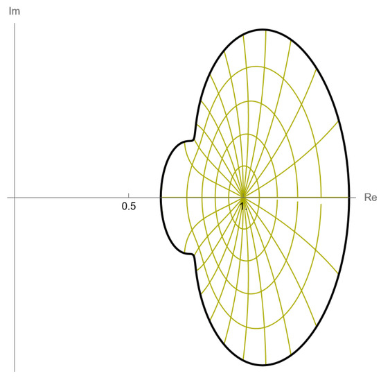
Figure 1.
Plot of the unit disk mapped under .
Motivated by these challenges, the present work aims to introduce two specific subclasses of univalent functions associated with a single-lobed elliptical domain, denoted as and , and to determine sharp bounds for their coefficients and the third-order Hankel determinant. This study extends the classical framework of starlike and convex functions by incorporating geometric considerations of the image domain. Meanwhile, the next two results establish explicit representation formulas for functions belonging to the classes and .
Theorem 1.
Let f be analytic in . Then if and only if
for some analytic function satisfying the subordination .
Proof.
Corollary 1.
Let g be analytic in . Then, if and only if
for some analytic function subordinate to .
Proof.
This result is an immediate consequence of the classical Alexander relation between the classes and . □
Below, we provide examples to demonstrate that the introduced classes are non-empty. These examples also serve to support the sharpness of the conjectures that will be presented in the coefficient estimation section.
Example 1.
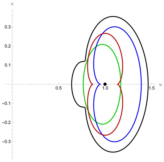
Let us define the following analytic functions:
It can be readily verified that and the image of over the unit disk satisfies for . Given that , this inclusion implies that for . Consequently, by invoking Theorem 1 and Corollary 1, it follows that the corresponding functions (or ), , defined accordingly, lie within the classes (or ) (as illustrated in Figure 2). The corresponding functions are given by
Furthermore,
Figure 2.
Plot boundaries of , , , as colors green, blue, red, and black, respectively.
Figure 2 below illustrates the required inclusion, demonstrating that the introduced function classes are non-empty.
Example 2.
The following formula yields an infinite number of functions:
belonging to . In particular,
Example 3.
The following formula yields an infinite number of functions:
belonging to , and
The qth Hankel determinant for analytic functions was introduced by Pommerenke [10] and is defined as
In general, sharp bounds for the second Hankel determinant
for various subclasses of univalent functions can often be derived relatively easily using standard techniques (see, e.g., [11,12,13,14,15,16,17,18,19,20]). However, determining sharp bounds for the third Hankel determinant
Since in this case, the formula simplifies to
The study of Hankel determinants, particularly of higher order, has gained increasing attention in geometric function theory due to their deep connections with coefficient problems and complex analytic structures. While the second Hankel determinant has been extensively analyzed for various subclasses of univalent functions, sharp bounds for the third-order determinant remain more challenging, motivating further investigation. Moreover, recent advances in defining univalent functions through image domains with specific geometric properties, such as elliptical regions, provide new opportunities to extend classical results (see [21,22,23]). To date, only a few sharp bounds have been obtained, while several non-sharp bounds for have been reported in the literature, e.g., [24,25,26,27,28,29]. Recently, some authors [30,31,32,33,34,35] have successfully established sharp estimates for in certain subclasses of univalent functions.
Despite previous studies providing both sharp and non-sharp estimates for the third-order Hankel determinant in various subclasses, precise bounds for functions associated with single-lobed elliptical domains remain unexplored. This motivates the present work, which aims to establish accurate coefficient bounds and determinant estimates, thereby contributing to a deeper understanding of univalent function theory in geometrically defined domains and laying the groundwork for further investigations.
2. Fundamental Lemmas
The fundamental lemmas serve as essential analytical tools for establishing the subsequent results. They provide core estimates and inequalities for the coefficients of functions belonging to the Carathéodory class , as given by the expression
which will be employed in proving the main results.
Lemma 1
Lemma 2
Lemma 3
Lemma 4
3. Estimate of 2nd Hankel Determinant
In this section, we aim to compute the initial coefficients for by determining their sharp bounds for both our classes.
Proof.
Let . Then,
for some Schwarz function .
It is possible to assume the existence of a function . Then, a well-known relation connects it to a Schwarz function, which can be expressed as follows:
Hence,
Substituting Equation (29) into Equation (28), and performing some simplifications, we obtain
Now, by comparing the coefficients of both sides of Equation (30), it follows that
These formulas express the initial coefficients explicitly in terms of the coefficients of the auxiliary function defined in Equation (29).
We can also rewrite Equation (33) in the following form:
Assuming and , the inequality is satisfied. Accordingly, using Equation (23), we obtain
Since
and
then, applying Equation (24) in Lemma 3, we obtain
The desired estimates are thus established. □
Motivated by the sharp bounds obtained for the initial coefficients, we propose the following conjecture for higher-order coefficients:
Conjecture 1.
Let . Then,
Proof.
Let . Then,
for some Schwarz function satisfying Equation (29). Substituting Equation (29) into Equation (35), followed by algebraic simplification, leads to
By comparing the corresponding coefficients of both sides in Equation (36), the following relations are obtained:
The remaining steps of the proof follow precisely the same framework employed in the proof of Theorem 2. In particular, the argument is completed by applying Lemmas 1–3 in the same logical order and deductive sequence. Hence, the structure of the proof is finalized, and its validity is thus established. □
We conclude this section by presenting the following conjecture, which arises naturally from the estimates established in the above theorem, reflecting the sharp estimates obtained for the initial coefficients and generalizing them to higher-order coefficients.
Conjecture 2.
Let . Then
In subsequent estimates, we examined sharp bounds of the second-order Hankel determinant for analytic classes (starlike and convex).
Theorem 4.
Let . Then
The sharpness is attained for the function given by Equation (10).
Proof.
Starting from the established coefficient relationships, we can express
By applying Lemma 4 with the substitutions , , and , we obtain
Applying the triangle inequality and taking absolute values leads to
In order to proceed, we aim to maximize . Differentiating with respect to y, we obtain
It is easy to verify that for . Therefore, the function attains its maximum at , which gives
Next, we determine the value of c that maximizes . Differentiating with respect to c, we find
Setting yields three roots: and two complex roots. Since is the only root in the interval and , the maximum occurs at . Thus, we obtain
This completes the argument, confirming the stated inequality. □
By adopting a reasoning analogous to that employed for the class , the proof for the class follows similarly. Hence, we state the result without providing the full proof.
Theorem 5.
After obtaining precise estimates for the initial coefficients and the second-order Hankel determinants, we naturally proceed to study the third-order Hankel determinants. This transition reflects the direct connection between the function coefficients and the associated geometric analyses, allowing for more complete and accurate results.
4. Third Hankel Determinants
In this section, we present a precise and systematic methodology for establishing the sharp upper bounds of the third-order Hankel determinants for both classes and . The approach adopted here carefully combines analytical techniques and the application of previously developed lemmas, aiming to provide a rigorous and comprehensive treatment of these extremal problems.
Theorem 6.
Proof.
Let . Given the rotational invariance of the class and the functional , it is permissible to restrict to the interval without loss of generality. Substituting Equations (31)–(34) into Equation (18), we arrive at
Before presenting the final expressions for , we decompose each contributing term by substituting the identities from Lemma 4 and the coefficient relations, resulting in the following detailed components:
for some such that .
After replacing with x, with y,and setting . Since the assumption that , then the expression simplifies to the following:
where
with
To accomplish this, the analysis must be conducted in three distinct parts: first, within the interior of the domain ; second, on its boundary faces; and finally, along its edges.
Case I: In order to examine how the function changes as y varies, we proceed by evaluating its partial derivative with respect to y:
Imposing the condition , we obtain
If is a critical point within , which possible only if
and
Now, only a solution that can meet both the inequalities in Equations (42) and (43) will be accepted as a critical point. Assuming and , which yields to is decreasing function, that is
Suppose . Thus, decreases over . Thus, , and a straightforward task illustrates that Equation (42) will not hold for all values of . This implies that we have not found a critical point for T in .
Case II: Interior of all six faces of the cuboid
(i) If , the function T reduces
then
which implies that has no optimal points in
(ii) If , we obtain
(iii) If , we get
then gives
The range of , if Also gives
Putting the value of y gives
Solving c within the range , we have . This indicates that the function has no optimal solution.
(iv) If , then the function T reduces
then gives the critical point , which yields that the maximum value of is (i.e., (
(v) If , the function T reduces
Thus
and
Computation shows that the system of equations and have no exact solution in
(vi) on the face , the function T reduces
Thus
and
Similar computation indicates that the system of equations and have no exact solution in
Case III: 12 edges of the cuboid
(i) If , then
for gives the critical point , where the max value is achieved as follows
(ii) , then
It is readily to show that , which indicates that the function is decreasing. Furthermore, the maximum value is accurate at
(iii) If , then
It is clear that , which shows that is increasing function and the max value is obtained, when
(iv) For and , it follows that
Setting , we obtain a critical point . At this value of c, the function reaches its highest value, which is
(v) If and , then
(vi) On , it follows that
(vii) If and , then
and computation generates that , which means is decreasing function and its maximum value achieves when ; that is,
(viii) On the edge and , then
For , we obtain a critical value , where the maximum value of is
Hence, we deduce that
Then, the value of inequality is
Thus, the inequality stands proven. □
Theorem 7.
Proof.
Assume that . Due to the rotational invariance of both the class and the functional , one may restrict the first coefficient to the range without loss of generality. By substituting Equations (37)–(40) into Equation (18), the expression for the Hankel determinant takes the form
Proceeding in a manner similar to the computations carried out in the proof of Theorem 6, and upon substituting , , and , we arrive at
where
with
By performing the calculations for the above equations and using the techniques adopted in Theorem 6, we arrive at
The proof is now complete. □
5. Conclusions
In this work, within the framework of Ma and Minda’s differential subordination and by introducing a novel lobed elliptical domain for the function , we have developed new subclasses of starlike and convex functions. Our analysis included deriving precise estimates for the initial coefficients up to the fifth order and determining sharp bounds for the second- and third-order Hankel determinants, verifying the sharpness of these results for both classes. Figure illustrations and analytical computations confirmed the non-emptiness of the introduced classes, highlighting the practical relevance of our approach. These results offer potential applications in geometric function theory, particularly in studying coefficient problems for complex analytic functions, as well as in computational and geometric modeling of analytic mappings. Furthermore, this study opens avenues for future research, including the exploration of additional subclasses associated with similar or more generalized domains, the investigation of higher-order Hankel determinants, and the integration of computational tools for broader experimental validation. The proposed domain can also be applied to other topics, such as those discussed in [42,43,44]. Overall, our findings contribute to advancing the understanding of geometric structures in analytic function theory and provide a foundation for subsequent theoretical and applied developments.
Author Contributions
Conceptualization, A.S.T. and S.H.H.; methodology, A.S.T., S.H.H. and A.A.; software, A.S.T., S.H.H. and A.A.; validation, A.S.T., S.H.H., A.A., M.A. and O.B.; formal analysis, A.S.T., S.H.H. and A.A.; investigation, A.S.T., S.H.H., A.A., M.A. and O.B.; resources, A.S.T., S.H.H. and A.A.; data curation, S.H.H.; writing—original draft preparation, A.S.T., S.H.H., A.A., M.A. and O.B.; writing—review and editing, A.S.T. and S.H.H.; visualization, A.S.T., S.H.H., A.A., M.A. and O.B.; supervision, A.S.T. and S.H.H.; project administration, S.H.H.; funding acquisition, A.S.T., S.H.H., M.A. and O.B. All authors have read and agreed to the published version of the manuscript.
Funding
This research was funded by the “1 Decembrie 1918” University of Alba Iulia through scientific research funds.
Institutional Review Board Statement
Not applicable.
Informed Consent Statement
Not applicable.
Data Availability Statement
No new data were created or analyzed in this study. Data sharing is not applicable to this article.
Acknowledgments
The researchers would like to express their sincere gratitude to the editors and reviewers for their valuable efforts that contributed to improving the quality of this manuscript.
Conflicts of Interest
The authors declare no conflicts of interest.
References
- Ma, W.; Minda, D. A unified treatment of some special classes of univalent functions. In Proceeding of the Conference on Complex Analysis; Li, Z., Ren, F., Yang, L., Zhang, S., Eds.; International Press: Cambridge, MA, USA, 1994; pp. 157–169. [Google Scholar]
- Mendiratta, R.; Nagpal, S.; Ravichandran, V. On a subclass of strongly starlike functions associated with exponential function. Bull. Malays. Math. Sci. Soc. 2015, 38, 365–386. [Google Scholar] [CrossRef]
- Goel, P.; Kumar, S.S. Certain class of starlike functions associated with modified sigmoid function. Bull. Malays. Math. Sci. Soc. 2020, 43, 957–991. [Google Scholar] [CrossRef]
- Mendiratta, R.; Nagpal, S.; Ravichandran, V. A subclass of starlike functions associated with left-half of the lemniscate of Bernoulli. Int. J. Math. 2014, 25, 1450090. [Google Scholar] [CrossRef]
- Raina, R.K.; Sokół, J. Some properties related to a certain class of starlike functions. Comptes Rendus Math. 2015, 353, 973–978. [Google Scholar] [CrossRef]
- Sharma, K.; Jain, N.K.; Ravichandran, V. Starlike functions associated with a cardioid. Afr. Math. 2016, 27, 923–939. [Google Scholar] [CrossRef]
- Tayyah, A.S.; Atshan, W.G. Starlikeness and bi-starlikeness associated with a new Carathéodory function. J. Math. Sci. 2025. [Google Scholar] [CrossRef]
- Mundalia, M.; Kumar, S.S. On a subfamily of starlike functions related to hyperbolic cosine function. J. Anal. 2023, 31, 2043–2062. [Google Scholar] [CrossRef]
- Tayyah, A.S.; Hadi, S.H.; Wang, Z.-G.; Lupaş, A.A. Classes of Ma–Minda type analytic functions associated with a kidney-shaped domain. AIMS Math. 2025, 10, 22445–22470. [Google Scholar] [CrossRef]
- Pommerenke, C. On the coefficients and Hankel determinants of univalent functions. J. Lond. Math. Soc. 1966, 14, 111–122. [Google Scholar] [CrossRef]
- Cho, N.E.; Kowalczyk, B.; Kwon, O.S.; Lecko, A.; Sim, Y.J. The bounds of some determinants for starlike functions of order α. Bull. Malays. Math. Sci. Soc. 2018, 41, 523–535. [Google Scholar] [CrossRef]
- Janteng, A.; Halim, S.A.; Darus, M. Coefficient inequality for a function whose derivative has a positive real part. J. Inequal. Pure Appl. Math. 2006, 7, 1–5. [Google Scholar]
- Lee, S.K.; Ravichandran, V.; Supramanian, S. Bound for the second Hankel determinant of certain univalent functions. J. Inequal. Appl. 2013, 2013, 281. [Google Scholar] [CrossRef]
- Raducanu, D.; Zaprawa, P. Second Hankel determinant for the close-to-convex functions. Comptes Rendus Math. 2017, 355, 1063–1071. [Google Scholar] [CrossRef]
- Sim, Y.J.; Lecko, A.; Thomas, D.K. The second Hankel determinant for strongly convex and Ozaki close-to-convex functions. Ann. Mat. Pura Appl. 2021, 200, 2515–2533. [Google Scholar] [CrossRef]
- Sokól, J.; Thomas, D.K. The second Hankel determinant for α-convex functions. Lith. Math. J. 2018, 58, 212–218. [Google Scholar] [CrossRef]
- Hadi, H.S.; Shaba, T.G.; Madhi, Z.S.; Darus, M.; Lupaş, A.A.; Tchier, F. Boundary values of Hankel and Toeplitz determinants for q-convex functions. MethodsX 2024, 13, 102842. [Google Scholar] [CrossRef] [PubMed]
- Hadi, S.H.; Darus, M.; Ibrahim, R.W. Hankel and Toeplitz determinants for q-starlike functions involving a q-analog integral operator and q-exponential function. J. Funct. Spaces 2025, 2025, 2771341. [Google Scholar] [CrossRef]
- Alsoboh, A.; Tayyah, A.S.; Amourah, A.; Al-Maqbali, A.A.; Al Mashraf, K.; Sasa, T. Hankel determinant estimates for bi-Bazilevič-type functions involving q-Fibonacci numbers. Eur. J. Pure Appl. Math. 2025, 18, 6698. [Google Scholar] [CrossRef]
- El-Ityan, M.; Sabri, M.A.; Hammad, S.; Frasin, B.; Al-Hawary, T.; Yousef, F. Third-order Hankel determinant for a class of bi-univalent functions associated with sine function. Mathematics 2025, 13, 2887. [Google Scholar] [CrossRef]
- Arif, M.; Abbas, M.; Alhefthi, R.K.; Breaz, D.; Cotîrlă, L.-I.; Rapeanu, E. Some analysis of the coefficient-related problems for functions of bounded turning associated with a symmetric image domain. Symmetry 2023, 15, 2090. [Google Scholar] [CrossRef]
- Arif, M.; Barukab, O.M.; Afzal Khan, S.; Abbas, M. The sharp bounds of Hankel determinants for the families of three-leaf-type analytic functions. Fractal Fract. 2022, 6, 291. [Google Scholar] [CrossRef]
- Peng, Z.; Arif, M.; Abbas, M.; Cho, N.E.; Alhefthi, R.K. Sharp coefficient problems of functions with bounded turning subordinated to the domain of cosine hyperbolic function. AIMS Math. 2024, 9, 15761–15781. [Google Scholar] [CrossRef]
- Bansal, D.; Maharana, S.; Prajapat, J.K. Third order Hankel determinant for certain univalent functions. J. Korean Math. Soc. 2015, 52, 1139–1148. [Google Scholar] [CrossRef]
- Raza, M.; Malik, S.N. Upper bound of the third Hankel determinant for a class of analytic functions related with lemniscate of Bernoulli. J. Inequal. Appl. 2013, 412, 8. [Google Scholar] [CrossRef]
- Zaprawa, P. Third Hankel determinants for classes of univalent functions. Mediterr. J. Math. 2017, 14, 1–10. [Google Scholar] [CrossRef]
- Zaprawa, P. Hankel determinants for univalent functions related to the exponential function. Symmetry 2019, 11, 211. [Google Scholar] [CrossRef]
- Shi, L.; Srivastava, H.M.; Arif, M.; Hussain, S.; Khan, H. An investigation of the third Hankel determinant problem for certain subfamilies of univalent functions involving the exponential function. Symmetry 2019, 11, 598. [Google Scholar] [CrossRef]
- Lupaş, A.A.; Tayyah, A.S.; Sokół, J. Sharp bounds on Hankel determinants for starlike functions defined by symmetry with respect to symmetric domains. Symmetry 2025, 17, 1244. [Google Scholar] [CrossRef]
- Banga, S.; Kumar, S.S. The sharp bounds of the second and third Hankel determinants for the class . Math. Slovaca 2020, 70, 849–862. [Google Scholar] [CrossRef]
- Kowalczyk, B.; Lecko, A.; Sim, Y.J. The sharp bound of the Hankel determinant of the third kind for convex functions. Bull. Aust. Math. Soc. 2018, 97, 435–445. [Google Scholar] [CrossRef]
- Kowalczyk, B.; Lecko, A.; Lecko, M.; Sim, Y.J. The sharp bound of the third Hankel determinant for some classes of analytic functions. Bull. Korean Math. Soc. 2018, 55, 1859–1868. [Google Scholar]
- Kwon, O.S.; Lecko, A.; Sim, Y.J. The bound of the Hankel determinant of the third kind for starlike functions. Bull. Malays. Math. Sci. Soc. 2019, 42, 767–780. [Google Scholar] [CrossRef]
- Lecko, A.; Sim, Y.J.; Smiarowska, B. The sharp bound of the Hankel determinant of the third kind for starlike functions of order 1/2. Complex Anal. Oper. Theory 2019, 13, 2231–2238. [Google Scholar] [CrossRef]
- Riaz, A.; Raza, M.; Thomas, D.K. The Third Hankel determinant for starlike functions associated with sigmoid functions. Forum Math. 2022, 34, 137–156. [Google Scholar] [CrossRef]
- Keogh, F.R.; Merkes, E.P. A coefficient inequality for certain classes of analytic functions. Proc. Am. Math. Soc. 1969, 20, 8–12. [Google Scholar] [CrossRef]
- Efraimidis, I. A generalization of Livingston’s coefficient inequalities for functions with positive real part. J. Math. Anal. Appl. 2016, 435, 369–379. [Google Scholar] [CrossRef]
- Ravichandran, V.; Verma, S. Bound for the fifth coefficient of certain starlike functions. Comptes Rendus Math. 2015, 353, 505–510. [Google Scholar] [CrossRef]
- Pommerenke, C. Univalent Functions; Vandenhoeck and Ruprecht: Göttingen, Germany, 1975. [Google Scholar]
- Libera, R.J.; Zlotkiewicz, E.J. Early coefficients of the inverse of a regular convex function. Proc. Am. Math. Soc. 1982, 85, 225–230. [Google Scholar] [CrossRef][Green Version]
- Kwon, O.S.; Lecko, A.; Sim, Y.J. On the fourth coefficient of functions in the Carathéodory class. Comput. Methods Funct. Theory 2018, 18, 307–314. [Google Scholar] [CrossRef]
- Rao, N.; Farid, M.; Jha, N.K. A study of (σ, μ)-Stancu-Schurer as a new generalization and approximations. J. Inequal. Appl. 2025, 2025, 104. [Google Scholar] [CrossRef]
- El-Ityan, M.; Amourah, A.; Hammad, S.; Buti, R.; Alsoboh, A. New Subclass of Bi-Univalent Functions Involving the Wright Function Associated with the Jung–Kim–Srivastav Operator. Gulf J. Math. 2025, 19, 451–462. [Google Scholar] [CrossRef]
- El-Ityan, M.; Al-Hawary, T.; Frasin, B.A.; Aldawish, I. A New Subclass of Bi-Univalent Functions Defined by Subordination to Laguerre Polynomials and the (p, q)-Derivative Operator. Symmetry 2025, 17, 982. [Google Scholar] [CrossRef]


Disclaimer/Publisher’s Note: The statements, opinions and data contained in all publications are solely those of the individual author(s) and contributor(s) and not of MDPI and/or the editor(s). MDPI and/or the editor(s) disclaim responsibility for any injury to people or property resulting from any ideas, methods, instructions or products referred to in the content. |
© 2025 by the authors. Licensee MDPI, Basel, Switzerland. This article is an open access article distributed under the terms and conditions of the Creative Commons Attribution (CC BY) license (https://creativecommons.org/licenses/by/4.0/).