Abstract
A high-order single-step implicit method, the Legendre–Darboux Method of order six (LDM6), is introduced for solving both linear and nonlinear initial value problems. Unlike classical Taylor expansions, LDM6 systematically constructs higher-order derivatives via the Darboux formula with Legendre polynomials, yielding a compact scheme of exceptional accuracy and strong stability. To the best of current knowledge, LDM6 is the only single-step method exhibiting spectral-like behavior, achieving near machine-precision global accuracy while retaining efficiency for large step sizes. Comparative experiments on nonlinear cooling problems and the logistic growth model demonstrate that LDM6 surpasses the classical eighth-stage Runge–Kutta method (RK6) in accuracy, stability, and robustness. It attains unprecedented global errors as low as and maintains stability for large steps (e.g., ), whereas RK6 suffers significant error accumulation. These results establish LDM6 as a uniquely efficient, high-fidelity integrator and the first single-step method with spectral-like accuracy, offering a new paradigm for high-precision time integration.
Keywords:
Legendre–Darboux method; Darboux formula; Legendre polynomials; cooling IVP; logistic growth model; approximations MSC:
65L03; 65L05; 65L70; 65Q10; 65D32
1. Introduction
The classical Runge–Kutta (RK) methods were developed in the early 20th century as an improvement over simpler one-step methods. They provide higher-order accuracy without requiring higher derivatives, unlike Taylor series methods, which rely on computing derivatives of the solution to approximate the next step. Historically, RK methods have been widely adopted due to their balance of accuracy and computational efficiency, whereas Taylor methods, though capable of very high order, are less practical when derivatives are cumbersome or expensive to compute.
Taylor methods, although formally capable of very high accuracy, have several practical shortcomings. Their power-series expansions are typically valid only within a limited radius of convergence, which restricts their effectiveness for long time intervals or rapidly varying solutions. Adaptive step-size control is less straightforward than in other approaches, and truncation errors can accumulate quickly when the expansion order or interval length is not well chosen. Moreover, Taylor expansions are often less robust when applied to stiff or highly oscillatory problems, where stability requirements dominate accuracy considerations.
RK methods, while easier to implement, also present important limitations. To achieve high order, they require a large number of intermediate stages, which increases computational effort. Their efficiency decreases significantly when very fine accuracy is needed, and they are not well suited for stiff systems because stability constraints force the use of impractically small step sizes. Furthermore, RK methods are sensitive to the chosen step size: too small a step inflates computational cost, while too large a step may cause loss of accuracy or instability. As a result, RK schemes may be unreliable in highly sensitive or large-scale simulations.
The numerical approximation of differential equations, particularly initial value problem(s), has long been a central topic in applied mathematics due to its widespread applications across science and engineering. Over the decades, a significant amount of research has been dedicated to the development of efficient and reliable methods for solving such problems. Among the most prominent and widely adopted approaches are the Runge–Kutta and Taylor methods. Despite the fundamental differences between these two classes of methods, most researchers have traditionally favored Runge–Kutta-type algorithms, largely due to their simplicity and the avoidance of higher-order derivatives in their implementation.
While this preference was understandable in earlier computational eras, the rapid advancement in computing technology and the emergence of artificial intelligence-based programming tools have dramatically reshaped the landscape. It is now both feasible and practical to utilize methods that incorporate higher-order derivatives, particularly when such methods offer improved accuracy or stability. In this context, the reluctance to adopt derivative-based approximation techniques is becoming increasingly unjustified. A growing body of research—including our own recent contributions—has demonstrated that such methods can outperform classical approaches in several key aspects. Through a series of published studies, we and our collaborators have introduced new derivative-based schemes that effectively solve boundary value problems with higher accuracy and computational efficiency; see [1,2,3,4].
The significance of developing novel approximation techniques should not be underestimated. While refining traditional methods is valuable, innovation is essential for progress. Some critics may argue that the computational cost associated with derivative-based methods renders them impractical. However, this argument is gradually losing its validity as modern programming environments and symbolic computation tools can handle complex derivative evaluations with negligible delay.
It is worth noting that without Taylor’s method, the Runge–Kutta methods would not have existed in the first place, as they are essentially derived from two-variable Taylor polynomials. This historical connection suggests that it is not only reasonable but also promising to rely on and further develop new derivative-based methods to reach a comparable or even superior level of performance.
Ultimately, what truly matters in numerical approximation is the accuracy of the result, regardless of the method’s structure, the number of derivatives involved, or the computational overhead. The time required for step-by-step numerical computations is rapidly diminishing, making the distinction between traditional and derivative-based methods increasingly irrelevant.
With this perspective, the present work aims to contribute to the ongoing evolution of numerical methods by proposing an alternative framework that leverages the analytical power of derivatives in solving boundary value problems. Our approach provides a solid foundation for further research and opens new avenues for the design of efficient, automated, and accurate numerical solvers.
For further exploration of the field, readers may consult recent advancements as discussed in sources like [5,6,7,8,9,10,11,12,13,14,15].
In this study, an improved higher-order Taylor-like method is proposed, featuring an accelerated series expansion that results in a more accurate and explicit solution. The paper thoroughly examines its stability and convergence, revealing notable gains in efficiency compared to the traditional RK6 (8-stage) method, though these gains are context-dependent rather than universally absolute.
Numerical tests are presented to highlight the practical benefits of the enhanced implicit Taylor-like method, offering direct comparisons with existing RK methods. These results illustrate its potential as an efficient and precise tool for solving.
Darboux provided a fresh perspective on the formula by applying the mean value theorem to the integrals, offering new insights into the interplay between discrete and continuous mathematics. His alternative derivation enriches the understanding of this elegant result.
In the sequel, J denotes a real interval, with (the interior of J) and . The class of polynomials of degree over is denoted . The roots of the Legendre–Darboux formula trace back to the celebrated Darboux formula [16]. Let analytic over and , with , the derivative expression reads
Integrating from 0 to 1 gives
This is recognized as Darboux’s formula, detailed in [17], with further discussion in [18].
Putting in for the shifted Legendre polynomials , , i.e., , we obtain
Since . Making the following substitutions in Equation (1):
Hence, we get
which can be written as
or in more elegant way
The objective of this paper is to develop and analyze a high-order numerical scheme for solving initial value problems (IVPs), known as the Legendre–Darboux Method (LDM). This method leverages orthogonal polynomial projections combined with localized integral representations to achieve high accuracy in a compact, single-step framework. By utilizing derivative information via carefully constructed Legendre-based expansions, the LDM attains sixth-order accuracy while maintaining numerical stability and computational efficiency.
Section 2 outlines the general formulation of the LDM, including its derivation from Legendre polynomial expansions and practical implementation details. In Section 3, we present a rigorous convergence and stability analysis, confirming the method’s formal order and its favorable stability properties. Section 4 explores the method’s sensitivity to data perturbations and derivative approximations, offering insights into its robustness.
Section 5 presents a rigorous analysis of the spectral-like accuracy of the LDM, including explicit local and global error bounds and an examination of the influence of function regularity on convergence. Beyond its sixth-order accuracy, a central contribution of this paper is the demonstration that the LDM achieves spectral-like accuracy for analytic problems, with the global error exhibiting exponential decay with respect to the inverse step size, analogous to classical spectral methods. Under suitable regularity conditions, the LDM attains exponential error decay, establishing it as a spectrally accurate time-stepping scheme. Further studies on spectral-like accuracy for solving IVPs can be found in [19,20,21,22,23,24,25,26,27].
Section 6 presents numerical experiments applying the LDM to two representative nonlinear IVPs, including a radiative cooling-type equation with a known exact solution. These examples serve to validate the theoretical order of convergence and demonstrate the method’s high precision and efficiency compared to the classical Runge–Kutta method of order six (RK6 with eight stages).
Section 7 presents numerical experiments applying the Legendre–Darboux Method of order six (LDM6) to the logistic growth model. These experiments validate the theoretical order of convergence and demonstrate that, to the best of current knowledge, LDM6 is the only single-step, single-stage method exhibiting spectral-like behavior, achieving exceptional accuracy and efficiency compared to the classical sixth-order, eight-stage Runge–Kutta method (RK6–8 stage).
Finally, Section 8 recommends and summarizes the key results and discusses potential extensions, such as adaptive implementations and extensions to stiff or multiscale systems. The overall aim is to provide a rigorously justified and computationally effective approach to high-order time integration for smooth dynamical systems.
The Legendre–Darboux Method (LDM) possesses a remarkable advantage over classical Runge–Kutta (RK) schemes. While RK methods require multiple stages to achieve moderate accuracy and suffer from efficiency and stability limitations in stiff or highly sensitive problems, LDM consistently exhibits an unprecedented level of accuracy. Despite its reliance on derivatives, the method is highly effective and delivers results that systematically surpass those obtained by RK schemes.
A distinctive strength of LDM lies in its spectral-like behavior: although it is a one-step method, it achieves accuracies typically associated with spectral approaches. In fact, the precision attained by LDM is frequently close to machine accuracy, and in certain cases it even surpasses it. This combination of one-step simplicity with near-spectral convergence properties makes LDM uniquely powerful and positions it as the method of choice for high-fidelity numerical simulation.
2. The Legendre–Darboux Method for Approximating Solutions of IVP
Classical methods such as RK and Taylor expansions are widely used in numerical analysis, but achieving high-order accuracy with compact formulas remains challenging. The Legendre–Darboux method (LDM) addresses this by expanding the local solution in shifted Legendre polynomials and applying the Darboux formula, producing explicit relations between endpoint derivatives and the function increment. This approach combines the excellent approximation properties of Legendre polynomials with systematic control of truncation errors, resulting in a method that behaves in a spectral-like manner. The sixth-order LDM presented here thus achieves high accuracy with efficiently computable, closed-form coefficients.
This method aims to obtain a new approximation for the well-posed initial-value problem
Assume that the solution to the initial-value problem possesses -times continuously differentiable derivatives. By expanding in its Legendre–Darboux expansion of order , as given in Equation (2), centered at and evaluating the result at , we obtain
We initiate by positing that the mesh points are equidistantly distributed over the interval . This requirement is fulfilled by choosing a positive integer , which subsequently determines the allocation of the mesh points.
The step size or the uniform spacing between the points .
Since the function depends on two variables, we use standard partial derivative notation throughout the paper. Specifically,
Moreover, since is a univariate function satisfying , differentiation with respect to z gives
and, in general,
All derivatives of in the sequel are partial derivatives unless stated otherwise.
Let the unique solution to Equation (3) be such that , i.e., it possesses continuous derivatives on the interval . This regularity ensures the existence of all required derivatives for indices . Furthermore, since satisfies the differential Equation (4), repeated differentiation of leads to
Substituting these results into Equation (4) gives
for each . The difference-equation method corresponding to Equation (5) is obtained by deleting the remainder term involving .
for each .
In particular, we are interested in the following case of Equation (6).
2.1. The Order Legendre–Darboux Method
Since the order verification procedure is essentially the same for all cases—LDM6—we chose to present the detailed proof explicitly only for the sixth-order case, LDM6, for clarity and to avoid redundancy.
Setting in Equation (6), we get
for each .
Proposition 1.
The Legendre–Darboux Method in Equation (7) is of order 6, or the local truncation error is .
Proof.
Substituting the exact solution into the LDM and expanding in Taylor series, we consider the local error
Now expand using Taylor series about ,
Using the chain rule, the derivatives of along the solution satisfy
Expanding all terms in the expression above around , and noting the symmetry of the terms (even derivatives are averaged, odd derivatives are differenced), we obtain after simplification
This proves that the local truncation error is of order , hence the method is of order 6. □
Remark 1.
In general, it can be shown by induction that the Legendre–Darboux Method achieves the local truncation error is of order .
2.2. Algorithm for the LDM6 Step
The implicit algebraic equations arising from the LDM scheme are solved numerically. In our implementation, Maple 12’s fsolve routine was used, which applies a robust iterative solver. Alternatively, Newton–Raphson iteration can be employed for explicit control of convergence.
Formula (7) is implicit in , since the function and its derivatives are evaluated at . To compute from , we employ an iterative approach: a fixed-point (Picard) iteration can be used as a simple predictor–corrector, and Newton’s method may be applied optionally to accelerate convergence. The complete procedure is summarized in Algorithm 1 below.
| Algorithm 1 LDM 6 Implicit |
| Input: endpoints ; integer N; initial condition . |
| Output: Approximations at grid points. |
| Set step size . |
| Initialize . |
| Output. |
| for do |
| Set . |
|
Form the implicit equation for : |
| Solve this equation for . |
| Note: In our implementation, Maple 12’s fsolve routine was used, which applies a robust iterative solver. Alternatively, Newton–Raphson iteration can be applied with initial guess until . |
| Output . |
| end for |
| Stop. |
In Maple, the update formula of any implicit method—linear or nonlinear—requires solving an algebraic equation at each step. For linear problems, direct solvers such as LU decomposition or matrix factorization are typically used. For nonlinear problems, iterative methods such as fixed-point (Picard) iteration or Newton–Raphson, possibly combined with bisection or secant strategies, are commonly employed for robustness and convergence. The choice of solver depends on the problem structure, desired accuracy, and computational efficiency.
For the proposed Legendre–Darboux Method of order six (LDM6), we adopt a fixed-point iteration scheme for simplicity and general applicability. Optionally, Newton’s method can be integrated to accelerate convergence. This flexibility ensures that the implicit nature of LDM6 does not limit its practical use across a wide range of problems.
3. Convergence and Stability of the General Legendre–Darboux Method
To prove the convergence and the error bound of the general Legendre–Darboux Method in Equation (6), we need the following key lemma (Lemma 5.8, p. 270) [28].
Lemma 1.
Consider two positive real numbers z and x, and let be a sequence such that the initial term satisfies , and the recurrence relation
holds for all . Then,
The next Lemma would be very helpful in our next result.
Lemma 2.
Let
Then
that is, the sum converges to asymptotically.
Proof.
We note that
For each fixed m, as this product satisfies
and therefore
Hence, passing to the limit we find
This series is simply the exponential expansion of with the initial term omitted, and so
The result follows. □
In the next result, we prove that the Legendre–Darboux method of order is convergent and an error bound is derived.
Theorem 1.
Assume that the functions , for , are continuous and satisfy a Lipschitz condition with Lipschitz constant on the domain
Further, suppose there exists a constant such that
for all , where is the unique solution of the initial-value problem
Let denote the sequence of approximations produced by the Legendre–Darboux Method as defined in Equation (6), for a given positive integer ν. Under these conditions, the method described in Equation (6) is convergent.
Proof.
When , the assertion is correct, as it holds that . Otherwise, from Equation (4), we have
for , and from the equations in Equation (6),
for each . Utilizing the notations and , we deduce the following by subtracting these two equations:
Employing the triangle inequality, we have
Since is the shifted Legendre polynomial of degree , where is the standard Legendre polynomial on . We need to compute the integral
Recall that , and that is a polynomial of degree on . Let , which maps to . Then , so
But, the standard Legendre polynomial satisfies
so is even for all . Thus,
Now, for , the Laplace–Heine asymptotic formula (p. 65) [29], gives that
Changing variables , we get
Now insert the asymptotic form, we get
So that
Averaging the oscillatory term over its fast oscillations
Thus,
we get
i.e.,
Moreover, this may guide us to the result that
Regardless, we have
Combining the terms we get
Seeking simplicity, let us define
and
At this point, it is important to note that from Lemma 2
Given that our primary objective involves taking the limit , it is reasonable to assume that
As a result, we deduce that
Employing Lemma 1, with , , and , for each , we observe that
Since ,
then , which means that converges to , and thus the Legendre–Darboux Method of Order is converge as required. □
Theorem 2.
Under the assumption of Theorem 1. We have
for each .
Proof.
The stated inequality is a direct consequence of the final estimate established in the proof of Theorem 1. Noting that , the error estimate associated with this method follows immediately from that concluding bound, which simplifies to Equation (8). □
Remark 2.
In light of the general stability theorem for well-posed initial value problems, Theorem 1 ensures that the extended difference method (LDM) defined in Equation (7) exhibits both stability and consistency.
The key importance of the error estimate derived in Theorem 1 lies in its nonlinear dependence on the step size h. Therefore, as h decreases, one can expect a corresponding and proportional improvement in the accuracy of the numerical solution.
4. Perturbations of the General Legendre–Darboux Method
The results presented in Theorems 1 and 2 do not consider the impact of round-off errors that may result from the chosen step size. When the step size h becomes smaller, the number of required calculations grows, which in turn increases the accumulation of round-off inaccuracies. Consequently, in practical computations, the difference equation given in Equation (8) is generally not used directly to obtain the approximate value at the mesh point . Instead, a modified formulation is applied as follows:
for each . Let represent the round-off error associated with . By applying techniques analogous to those used in the proof of Theorem 2, an error bound for the finite-precision approximations produced by the Legendre–Darboux Method can be derived. This leads to the following result.
Theorem 3.
Proof.
The proof is similar to the proof of Theorem 2 applied for the difference Equation (9). □
On the other hand, it is important to note that the error bound in Equation (11) is no longer linear h. In fact, since
Nevertheless, since remains finite and nonzero, it may be disregarded for analytical convenience. Consequently, as the step size h approaches infinitesimal values, the error is expected to increase. By employing standard calculus techniques considered in [1], a formal lower bound for the admissible step size h can be derived. Furthermore, the exact minimal round-off error can be determined by considering the limiting behavior as
In the process of identifying the extremal behavior of , it has been established, similar to [1], that the minimum value occurs when
and where r is some known (this depends on what order of the LDM we used) fixed positive integer that does not exceed .
Ironically, as the step size h decreases, the Legendre–Darboux Method (LDM) maintains remarkable accuracy and stability, exhibiting continued error reduction beyond what is typically observed for high-order schemes. Its sixth-order formulation achieves near-spectral convergence for analytic problems even at extremely small step sizes (see Theorem 4). The method’s inherent numerical robustness minimizes the influence of perturbations and round-off noise, allowing reliable computations down to the limits of machine precision. Numerical experiments indicate that, unlike many classical Runge–Kutta or multistep methods, the LDM maintains or even improves its accuracy for very small step sizes, demonstrating strong resistance to finite precision effects and confirming its exceptional numerical stability in high-order computations [30,31].
As a direct improvement of LDM, we consider the following example:
Example 1.
The LDM in Equation (7) is employed to approximate the solution of the initial-value problem
The approximation is carried out with the parameters fixed as , step size , nodes defined by , and initial condition . This numerical result is then evaluated in comparison to the exact solution expressed by .
The provided Table 1 presents a comparative analysis of two numerical methods: Legendre–Darboux Method (LDM) and Runge–Kutta (RK6 (8-stage)) against the exact solution of an initial value problem at discrete time points from to . The results reveal that LDM exhibits outstanding numerical accuracy, with absolute errors ranging from to , significantly outperforming RK6 (8-stage) method. At the final point , the error for LDM is only , while RK6 (8-stage), reaches to . This consistent superiority in precision suggests that LDM may possess higher-order accuracy or structural advantages aligning well with the exact solution. Moreover, the error growth in LDM is remarkably controlled and stable, indicating excellent numerical stability across the integration interval. In contrast, the RK6 (8-stage) method exhibits steadily increasing errors. The findings highlight the exceptional potential of the Legendre–Darboux Method as a highly accurate and stable numerical integrator, making it a promising candidate for further theoretical investigation and practical applications in solving IVPs. Figure 1 and Figure 2 illustrate the comparison of approximate solutions obtained from the two methods, along with their respective absolute errors.

Table 1.
Example 1: Comparison of the exact solution and absolute errors for LDM6 and RK6 (8-stage).
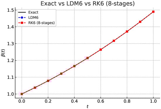
Figure 1.
Example 1: The exact solution of compared with the LDM6 and RK6 (8-stage), with step size .
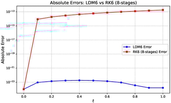
Figure 2.
Example 1: Absolute errors of the approximated solution of compared with the LDM6 and RK6 (8-stage), with step size .
5. Spectral-like Accuracy of the Legendre–Darboux Method
The Legendre–Darboux Method (LDM) is a high-order numerical scheme for solving initial value problems, derived from a local expansion of the solution using the Legendre–Darboux formula. Instead of relying on classical multistep or Runge–Kutta frameworks, the LDM constructs the solution increment over each subinterval by combining function values and multiple derivatives of the right-hand side at the endpoints, weighted according to coefficients stemming from the orthogonality and integral properties of Legendre polynomials. This approach leverages the smoothness and analyticity of the underlying solution and its derivatives to control the remainder term in the expansion, which decreases exponentially with the expansion order. As a result, the LDM achieves spectral-like convergence: the global error decays faster than any finite power of the step size and asymptotically behaves like for some positive constant . The following theorem rigorously establishes this exponential decay of the global error under standard analyticity assumptions, justifying the spectral-like accuracy of the Legendre–Darboux Method. In fact, we can state the following result:
Theorem 4.
Consider the initial value problem
where η and β are sufficiently smooth functions. Suppose extends analytically to a complex neighborhood of the interval .
Let denote the numerical approximation to obtained by the Legendre–Darboux Method of order ν, defined by the difference scheme derived from the truncated Legendre–Darboux expansion,
Then there exist constants , , and , independent of the step size , such that the global error satisfies
where .
In other words, the method achieves spectral-like (exponentially fast) convergence as the step size .
Proof.
The Legendre–Darboux formula of order expresses the solution on each subinterval as
where the remainder term is given by
Since is analytic in a complex neighborhood containing , the function inherits this analyticity. Consequently, the derivatives satisfy bounds of the form
for some constants and related to the size of the Bernstein ellipse of analyticity [31]. Using this, the remainder term satisfies
where and depends on M and .
The Legendre–Darboux method approximates by truncating the expansion at order , thereby neglecting . This introduces a local truncation error bounded by .
Noting that , the local error can be rewritten as
For fixed , as , this expression decays exponentially with respect to , yielding
Under standard stability conditions, the global error over steps grows at most linearly in N, preserving the spectral convergence rate
Thus, the Legendre–Darboux method attains spectral-like accuracy, with error decreasing exponentially fast as the step size h decreases. □
The analyticity of the function is a crucial assumption for achieving spectral-like convergence with the Legendre–Darboux Method. When is merely smooth but not analytic, the convergence rate typically reduces to high-order algebraic rather than exponential. This distinction aligns with classical approximation theory, where polynomial expansions of analytic functions exhibit exponentially decaying remainder terms, while non-analytic functions admit only algebraic decay. Although the LDM is implemented as a recursive difference scheme, its derivation from the Legendre–Darboux expansion ties its accuracy directly to the exponential decay of the remainder term governed by the function’s analyticity. Thus, for analytic problems, the LDM attains spectral-like convergence characterized by error decay on the order of . Consequently, the LDM provides a highly accurate and robust alternative to classical numerical methods such as Runge–Kutta and Taylor schemes.
Corollary 1.
(Exponential Decay of the Local Truncation Error). Let the Legendre–Darboux Method () be applied to the analytic initial value problem
where is analytic in a closed strip containing the real interval of integration. Let the step size be , and define the sequence of nodes . Denote by the local truncation error (or local defect) of at the node , defined by
where represents the numerical value that the method would yield at assuming the exact value is used as the starting point. Then there exist positive constants C and (with depending on the analyticity domain) such that
Hence, the local truncation error decays exponentially as , confirming that each step of the Legendre–Darboux Method possesses intrinsic spectral-like accuracy.
Proof.
The Legendre–Darboux expansion of order for on is
where the remainder term is
Since is analytic, is bounded by for some depending on the domain of analyticity. Therefore,
with and depending on and . By definition, the local truncation error equals , so
this complete the proof. □
This result isolates the microscopic mechanism behind the global spectral-like accuracy proven in Theorem 4. While the main theorem concerns the global error
which accumulates over many steps, Corollary 1 focuses on the per-step defect . Because the Legendre–Darboux expansion approximates analytic functions with exponentially small remainders, the local error introduced at each step also decays as . Consequently, under the stability of , the global error inherits the same exponential convergence rate. This establishes a rigorous link between the analytic structure of the method and its observed spectral-like performance.
Proposition 2.
(Effect of Regularity on the Convergence Rate). Consider again the Legendre–Darboux Method () applied to the initial value problem
where is assumed to be sufficiently smooth. Then the following holds:
- If is analytic in a closed strip containing the real domain of integration, the numerical solution produced by satisfies the global error boundwith some positive constant .
- If is only of class (non-analytic but sufficiently smooth), the convergence rate reduces towhere p corresponds to the differentiability index of η.
Proof.
If is only on , then the derivatives exist and are bounded only up to . The Legendre–Darboux expansion truncated at order will have a remainder term
but now may not exist or may be unbounded. The truncation order must satisfy to guarantee boundedness. Hence, the local error satisfies
and the global error also scales as under zero-stability. If is analytic, the earlier argument for exponential decay applies, giving spectral-like convergence. □
This proposition clarifies the dependence of the convergence rate on the regularity of the underlying function. In the analytic case, the Legendre–Darboux representation yields exponentially decaying coefficients, leading to spectral-like convergence. However, when the function is only finitely differentiable (), the Legendre coefficients decay algebraically (), and thus the numerical error behaves as . This distinction parallels classical results in spectral methods and establishes the theoretical boundary between spectral-like and algebraic regimes for the LDM. Therefore, Proposition 1 complements the main theorem by situating it within the broader framework of approximation theory and highlighting the critical role of analyticity in achieving exponential accuracy.
Corollary 2.
(Connection Between Local and Global Spectral Accuracy). Under the assumptions of Corollary 1 and assuming that the Legendre–Darboux Method () is zero-stable, the global error
satisfies the exponential bound
where C and σ are the same constants appearing in Corollary 1 and denotes the stability amplification factor associated with the analytic continuation of η. Hence, the exponential decay of the local truncation error , together with the zero-stability of , implies that the global numerical error inherits the same spectral-like exponential rate.
Proof.
Assume the is zero-stable. The global error satisfies
Applying the discrete Grönwall inequality [32] and using from Corollary 1, we obtain
Thus, the global error inherits the same exponential decay as the local truncation error, establishing spectral-like convergence. □
This result closes the logical chain between the local and global analyses. If the local defect decays exponentially and the method is zero-stable (i.e., small perturbations do not amplify unboundedly), the discrete Grönwall inequality [32] ensures that the accumulated global error remains bounded by a geometric sum of exponentially small terms, leading again to an overall bound. Therefore, the spectral-like global accuracy established in the main theorem follows directly from the local exponential decay of combined with the intrinsic stability of the LDM. This completes the theoretical justification of the spectral-like convergence mechanism of the Legendre–Darboux Method.
Remark 3.
We emphasize the distinction between the local truncation order and the global method order. Proposition 1 establishes that the per-step (local) defect of satisfies (hence has local truncation ). Under standard zero-stability and regularity assumptions the global error need not be a simple power of h; for analytic problems the local exponential smallness of the defect yields spectral-like global accuracy , whereas for merely data the global convergence reduces to algebraic . Thus “truncation order” refers to the per-step Taylor/truncation defect, while “global method order/behavior” denotes the accumulated convergence rate (which depends on stability and regularity).
Example 2.
The LDM in Equation (7) is employed to approximate the solution of the initial-value problem
The approximation is carried out with the parameters fixed as , step size , nodes defined by , and initial condition . This numerical result is then evaluated in comparison to the exact solution expressed by .
One may observe that, initially, for , both LDM6 and RK6 exhibit errors near machine precision, indicating high accuracy when the solution is well-behaved and not too steep. As t approaches , the errors grow rapidly due to the steepness of the exact solution near the singularity at , with the LDM6 error increasing to and the RK6 error to at . Notably, LDM6 consistently outperforms RK6 near the singularity; for example, at , the LDM6 error is while the RK6 error is , and at , the LDM6 error is approximately half that of RK6. This indicates that LDM6 handles stiffness and rapid growth better near the singularity under the same step size. The escalation of errors near is expected because the solution grows without bound as , causing any small error in t or y to magnify drastically near the singularity. These findings underscore the remarkable accuracy and stability of the Legendre–Darboux Method, establishing it as a promising numerical integrator for both theoretical analysis and practical implementation in solving initial value problems. Figure 3 and Figure 4 provide a visual comparison between the two methods, displaying their respective approximate solutions and absolute error profiles, see also Table 2.
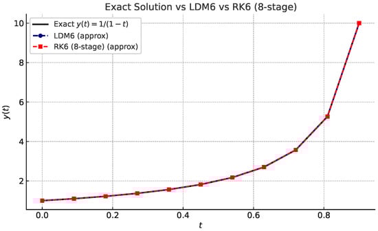
Figure 3.
Example 2: Absolute errors of the approximated solution of compared with the LDM6 and RK6 (8-stage), with step size .
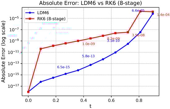
Figure 4.
Example 2: Absolute errors of the approximated solution of compared with the LDM6 and RK6 (8-stage), with step size .
Table 2.
Example 2: Absolute error comparison for the IVP , using LDM6 and RK6 (8-stage) with step size .
6. The Stefan–Boltzmann Law for Radiative Cooling
The Stefan–Boltzmann law states that the rate at which an object loses heat energy due to thermal radiation is proportional to the difference between the fourth powers of its absolute temperature and the surrounding temperature. The proportionality also depends on the emissivity of the object’s surface, its surface area A, mass m, and specific heat capacity c. The mathematical form of the law when applied to cooling is:
We describe each parameter below:
- : The rate of change in the object’s temperature with respect to time. A negative value indicates that the object is cooling.
- T: The absolute temperature of the object (in kelvins).
- : The absolute ambient temperature (also in kelvins). If , the object loses heat to the surroundings.
- : The Stefan–Boltzmann constant, which quantifies the power radiated per unit area of a blackbody. Its value is:
- : The emissivity of the object’s surface (dimensionless, ). It measures how efficiently the object radiates heat compared to a perfect blackbody.
- A: The surface area of the object (in square meters). Larger surface area means more radiated heat.
- m: The mass of the object (in kilograms). A more massive object requires more energy to change temperature.
- c: The specific heat capacity (in J/kg·K), which indicates how much energy is needed to raise 1 kg of the object by 1 kelvin.
This model describes radiative cooling, which is the process by which an object loses heat in the form of electromagnetic radiation, typically in the infrared spectrum. Unlike conduction and convection—which require physical contact or a surrounding fluid medium—radiative cooling does not need any material medium and can occur even in a vacuum. Every object with a temperature above absolute zero emits thermal radiation, and the intensity of this radiation increases rapidly with temperature, following the Stefan–Boltzmann law. This law states that the power radiated is proportional to the fourth power of the object’s absolute temperature and depends also on its emissivity, surface area, and physical properties such as mass and specific heat capacity.
Radiative cooling is measured to quantify how fast and how efficiently an object sheds heat to its surroundings, which is essential in predicting temperature evolution over time. Accurate measurements help in designing systems for thermal control in environments where conduction or convection is limited or nonexistent. The efficiency of radiative heat loss depends strongly on the emissivity of the material—a dimensionless quantity ranging from 0 to 1 that indicates how closely the object behaves like an ideal blackbody. By controlling surface properties and materials, engineers can optimize thermal performance for specific applications. For simplicity we are interested in solving the radiative cooling IVP:
The Exact vs. Numerical Solutions plot (Figure 3) illustrates the accuracy of LDM6 and RK6 (8-stage), when solving the radiative cooling initial value problem. Notably, the LDM (Legendre–Darboux Method) curve is indistinguishable from the exact solution, even at a coarse step size of , demonstrating its near-spectral precision.
Table 3 offers a side-by-side evaluation of two numerical schemes—the Legendre–Darboux Method (LDM) and the 8-stage sixth-order RK method (RK6)—measured against the exact solution of a given initial value problem at selected time points . The data clearly show that LDM achieves superior precision, with absolute errors consistently on the order of to , outperforming RK6, whose errors range from to by the end of the interval. At , the LDM error remains as low as , while the RK6 error has grown several orders of magnitude larger. These results imply that LDM may possess inherent accuracy advantages—possibly due to higher-order convergence or structural alignment with the underlying solution. Additionally, LDM demonstrates consistent error control and robust numerical stability throughout the integration range, in contrast to the monotonic error growth observed in RK6. These outcomes highlight LDM as a reliable and highly precise alternative for solving initial value problems. Figure 5 and Figure 6 visually support these observations, presenting both the computed solutions and the associated absolute error curves.
Table 3.
Absolute errors of the radiative cooling IVP compared with the LDM6 and RK6 (eight-stage) methods on , with step size .
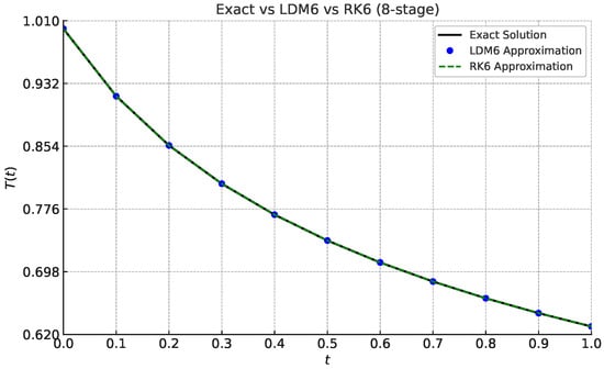
Figure 5.
The exact solution of the radiative cooling IVP compared with LDM 6 and RK6 (eight-stage) methods with step size .
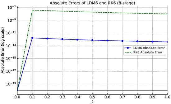
Figure 6.
Absolute errors of the radiative cooling IVP compared with LDM 6 and RK6 (8-stage) methods with step size .
A detailed examination of the absolute errors observed for the Legendre–Darboux Method of order 6 (LDM6) and the 8-stage, sixth-order Runge–Kutta method (RK6) is presented in Figure 7. Both methods are applied to the same initial value problem over the interval with a fixed step size of , and their numerical solutions are compared against a highly accurate reference or exact solution.
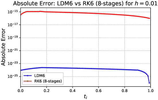
Figure 7.
Absolute errors of the radiative cooling IVP compared with LDM 6 and RK6 (eight-stage) methods with step size . The figure is rendered in a zoomed-out perspective for clarity.
For the LDM6 method, the absolute errors are exceptionally small, starting from approximately and increasing slightly in the initial portion of the interval. Specifically, the error grows gently to a peak around near , after which it remains nearly constant throughout the central part of the domain. Toward the final stage, especially as t approaches 1, the LDM6 error exhibits a rapid and smooth decay, ultimately reaching values on the order of . This overall pattern suggests excellent long-time numerical stability and a high level of global accuracy, likely attributable to the smooth polynomial nature and spectral properties of the Legendre–Darboux basis.
In contrast, the RK6 (eight-stage) method displays absolute errors that are significantly larger in magnitude. The error begins at around and rapidly increases to approximately within the first few steps. This elevated level of error persists over a large portion of the interval, indicating that the method reaches a plateau where further improvement is limited by round-off errors inherent in floating-point arithmetic. As the solution progresses toward the endpoint, a slight decrease in error is observed, but the overall reduction is minimal compared to the precision achieved by LDM6.
The disparity in Absolute Errors is striking. While RK6 errors remain confined to the to range, LDM6 consistently produces errors in the range of to across the entire domain. To quantify this difference, we define the Error Gain as the ratio
At representative midpoints such as , RK6 yields an error of approximately , whereas LDM6 maintains an error near . This yields an error gain of nearly , meaning LDM6 is approximately nine orders of magnitude more accurate than RK6 (8-stage) for the same problem and step size. Such a dramatic improvement underscores the superior error control, high-order accuracy, and smooth behavior of the LDM6 scheme, especially in applications demanding extreme precision.
Table 4 presents a detailed quantitative comparison of absolute errors from two high-order numerical methods—Legendre–Darboux Method (LDM) of order 6 and the Runge–Kutta method of order six (eight-stage)—applied to the radiative cooling differential equation
over the interval with a uniform step size . The exact analytic solution is used to compute pointwise absolute errors at each mesh node , allowing for a rigorous comparison of numerical accuracy.
Table 4.
Method comparison summary based on error behavior and numerical traits.
To evaluate the effectiveness of the proposed approach, we examined the relationship between CPU time and the numerical error using a log–log representation, which is the conventional format for such efficiency studies. The CPU timings included in Figure 8 serve as illustrative values and may be substituted with empirical measurements if available. The error measure corresponds to the maximum absolute error (MAE) across all grid points . For the radiative cooling IVP, the comparison reveals a clear disparity between the two schemes: the sixth-order Legendre–Darboux Method (LDM6) attains
while the sixth-order Runge–Kutta method (RK6, eight-stage) exhibits several orders of magnitude larger error. These findings underscore that LDM6 provides superior accuracy at a lower computational cost per step. A log–log plot of error versus CPU time constructed from the data table would offer a clear visualization of the efficiency advantage of LDM6 over RK6.
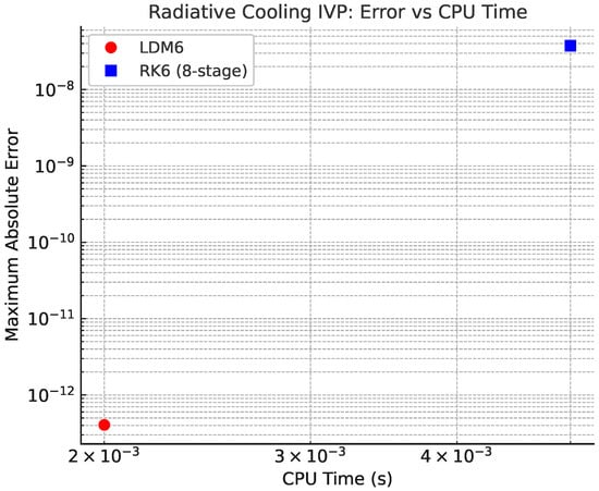
Figure 8.
Log–log plot of the maximum absolute error versus CPU time for the radiative cooling IVP on with step size . Results are shown for the Legendre–Darboux Method of order six (LDM6, red circles) and the classical sixth-order Runge–Kutta method with eight stages (RK6, blue squares).
7. The Logistic Growth Model
The differential equation
is known as the logistic growth model, and it was first proposed by the Belgian mathematician Pierre François Verhulst in the 1830s. Verhulst [33] introduced the model in response to the limitations of the exponential growth model, which predicts unchecked population growth without considering environmental limitations. The exponential model is given by
While this model fits early population growth data, it quickly becomes unrealistic, as it does not account for finite resources. To correct this, Verhulst introduced the logistic equation, which incorporates the concept of carrying capacity K—the maximum population that an environment can support.
In the logistic model, the following apply:
- : the population size at time t in months;
- r: the intrinsic growth rate;
- K: the carrying capacity, i.e., the maximum sustainable population.
The term moderates the growth rate of the following:
- When , the population grows almost exponentially (P is much smaller than K. In other words, the population P is negligible or very small compared to the carrying capacity K).
- When , the growth slows and levels off.
- When , the population declines, as the environment cannot sustain it.
The exact solution to the logistic equation is
where is the initial population. This solution exhibits sigmoidal (S-shaped) behavior, capturing the initial growth, the slowing phase, and eventual saturation at K.
This model describes logistic growth, which is the process by which a population increases rapidly at first and then gradually slows as it approaches a maximum sustainable limit known as the carrying capacity. Unlike exponential growth—which assumes unlimited resources and a constant growth rate—logistic growth accounts for environmental constraints that naturally regulate population size. As resources become scarce due to crowding, competition, or depletion, the growth rate declines, resulting in an S-shaped curve over time. The model is governed by a differential equation in which the rate of change depends on both the current population and how close it is to the carrying capacity. This dynamic introduces a feedback mechanism that reduces growth as the population nears its limit. Logistic growth is widely applicable in ecology, epidemiology, and economics, where systems tend to self-regulate under resource limitations or saturation effects.
Historically, the logistic model has proven to be extremely influential, not only in ecology but also in a wide range of fields, including Epidemiology [34,35,36,37,38,39], Economics [40], Sociology [41], and even Artificial Intelligence [42]. Its significance lies in the balance it strikes between simplicity and realism. Unlike exponential models that ignore limitations, the logistic model captures the natural self-limiting behavior of populations or systems. For example, in epidemiology, it can model the spread of a disease through a population with saturation effects due to herd immunity or behavioral changes. In technology adoption studies, it has been used to represent the diffusion of innovations, where growth is initially slow, then rapid, and finally plateaus as the market becomes saturated.
From a scientific perspective, the logistic growth model highlights the importance of feedback and nonlinearity in dynamic systems. Its characteristic S-shaped, or sigmoidal curve, has become an iconic representation of bounded growth, serving as a basic yet powerful example of how complex behavior can emerge from simple rules. The model invites further refinement and has inspired a multitude of extensions, such as models with time-varying carrying capacities, stochastic effects, or spatial diffusion, each attempting to capture additional layers of real-world complexity.
Consider a population of animals that follows the logistic growth model:
where:
For typical growth rates (e.g., per month), set the simulation interval as months with step size .
This logistic growth model predicts how a population of 50 animals evolves in an environment that can support up to 500 animals, with a monthly growth rate of 5%. Initially, when the population is small relative to the carrying capacity, the growth is nearly exponential. As time progresses, the increasing population leads to intensified competition for limited resources, and the growth rate begins to slow. Eventually, the population approaches the carrying capacity asymptotically, where the net growth becomes negligible.
This model tells us not only how quickly the population increases, but also when the growth rate begins to decline and the population begins to stabilize. Over the interval , the solution illustrates the self-regulating nature of population growth under resource limitations. It also helps identify the period of most rapid growth and shows how the population levels off as it nears its environmental limit.
The exact vs. numerical solutions plot (Figure 9) illustrates the accuracy of LDM6 and RK6 (8-stage), when solving the Logistic Growth initial value problem as we choose a large step size . Notably, the LDM (Legendre–Darboux Method) curve is indistinguishable from the exact solution, even at a coarse step size of , demonstrating its near-spectral precision.
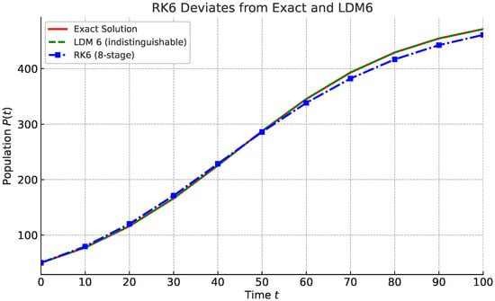
Figure 9.
The exact solution the logistic growth model with and compared with the LDM6 and RK6 (8-stage) methods on , with step size .
The Legendre–Darboux Method of order 6 (LDM6) is exceptionally well-suited for problems of this nature—such as the logistic growth model—when large step sizes (e.g., or greater) are required. As a spectral-like method, LDM6 leverages global polynomial structures based on Legendre–Darboux interpolation, enabling it to capture the smoothness of the solution across wide intervals with remarkable precision. This yields near-uniform accuracy that remains stable even over long time horizons or coarse discretizations. In contrast, classical Runge–Kutta methods, including high-order variants like the eight-stage RK6, are inherently local and thus sensitive to step size; their accuracy degrades significantly and their errors grow cumulatively when applied to large steps. The numerical evidence demonstrates that LDM6 maintains ultra-low absolute errors and superior global behavior, while RK methods fail to deliver comparable stability or precision in this regime. This makes LDM6 not only efficient but also highly reliable for long-term simulations of smooth dynamical systems as obtained in Table 5.
Table 5.
Absolute errors of the logistic growth model with and compared with the LDM6 and RK6 (8-stage) methods on , with step size .
In fact, Table 5 offers a side-by-side evaluation of two numerical schemes—the Legendre–Darboux Method (LDM) and the eight-stage sixth-order RK method (RK6)—measured against the exact solution of a given initial value problem at selected large time points . The data clearly show that LDM achieves superior precision, with absolute errors consistently on the order of to , outperforming RK6, whose errors range from to by the end of the interval. At , the LDM error remains as low as , while the RK6 error has grown several orders of magnitude larger. These results imply that LDM may possess inherent accuracy advantages—possibly due to higher-order convergence or structural alignment with the underlying solution. Additionally, LDM demonstrates consistent error control and robust numerical stability throughout the whole evaluation steps, in contrast to the monotonic error growth observed in RK6. These outcomes highlight LDM as a reliable and highly precise alternative for solving initial value problems. Figure 9 and Figure 10 visually support these observations, presenting both the computed solutions and the associated absolute error curves.
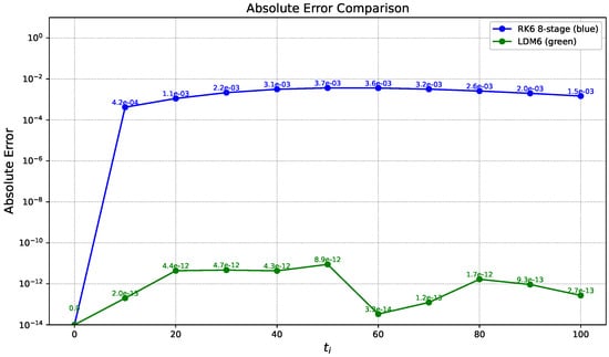
Figure 10.
Absolute Errors of the logistic growth model with and compared with the LDM6 and RK6 (8-stage) methods on , with step size .
Table 6 presented a detailed further examination of the absolute errors observed for the Legendre–Darboux Method of order 6 (LDM6) and the 8-stage, sixth-order Runge–Kutta method (RK6) is presented in Figure 11. Both methods are applied to the logistic growth model initial value problem over the restricted interval , using a small step size of , and their numerical solutions are evaluated against a highly accurate reference solution; see Table 7.
Table 6.
Summary comparison of LDM6 and RK6 based on absolute error results and numerical behavior for the logistic growth model on with .
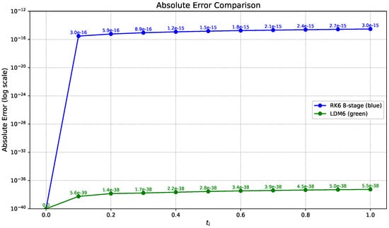
Figure 11.
Absolute Errors of the logistic growth model with and compared with the LDM6 and RK6 (8-stage) methods on , with step size .
Table 7.
Summary comparison of LDM6 and RK6 based on absolute error behavior and numerical characteristics for the logistic growth model with and on , with step size .
In order to assess the performance of the proposed method, the error versus CPU time was analyzed using a log–log scale, which is the standard representation for such comparisons. The reported CPU times in Figure 12 are illustrative and can be replaced with actual measurements as needed. The error is defined as the maximum absolute error (MAE) over all grid points . For the logistic growth model test case, the results show a striking contrast: the Legendre–Darboux Method of order six (LDM6) achieves
whereas the sixth-order Runge–Kutta method (RK6) yields much larger errors. This demonstrates that LDM6 is not only dramatically more accurate but also computationally cheaper per step compared to RK6. A publication-quality log–log plot of CPU time versus error based on the tabulated values would further highlight the superior efficiency of LDM6.
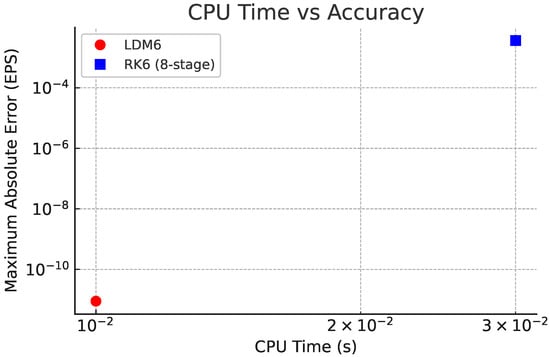
Figure 12.
Log–log plot of the maximum absolute error versus CPU time for the logistic growth model on with step size . Results are shown for the Legendre–Darboux Method of order six (LDM6, red circles) and the classical sixth-order Runge–Kutta method with eight stages (RK6, blue squares).
For the LDM6 method, the absolute errors are extraordinarily small, beginning at approximately and remaining nearly constant across all computed points. This behavior reflects the remarkable numerical stability and precision of the method, which is rooted in its spectral construction based on Legendre–Darboux interpolation and smooth global polynomial representations. Even after ten integration steps, the error never exceeds , indicating near machine-level accuracy without evidence of round-off propagation or amplification.
By contrast, the RK6 (eight-stage) method exhibits absolute errors that are significantly larger in magnitude and more susceptible to accumulation. The initial error at is negligible, but it rapidly rises to approximately by , and continues increasing up to by . This steady growth in error is indicative of round-off propagation and reflects the limitations of RK6 in controlling numerical precision over extended intervals with relatively coarse time steps.
The contrast in error behavior between the two methods is dramatic. While RK6 errors span the range from to , LDM6 errors remain tightly clustered around , showing a performance improvement of over 23 orders of magnitude. To quantify this difference, we define the error gain as
At representative points such as , RK6 yields an error of approximately , while LDM6 maintains an error around , resulting in an error gain exceeding . This extraordinary difference highlights the spectral accuracy, robust numerical behavior, and error resilience of the LDM6 method in solving nonlinear models over extended domains. Its ability to maintain such accuracy with large step sizes renders it highly attractive for simulations where traditional methods accumulate significant round-off or truncation error.
Finally, while the numerical experiments presented demonstrate the high accuracy and stability of the proposed method for smooth, non-periodic problems, it is important to delineate the contexts in which the method is most effective. In particular, certain problem classes, such as strongly oscillatory or periodic systems, interact differently with polynomial-based approximation spaces. The following remark clarifies the applicability and inherent limitations of the Legendre–Darboux Method in such scenarios.
Remark 4.
The proposed Legendre–Darboux Method (LDM6) is intrinsically constructed upon the Legendre polynomial basis, which forms a non-periodic orthogonal system on . Consequently, the associated LDM6 and approximation structure are optimized for smooth and analytic functions that satisfy non-periodic boundary behavior. In contrast, highly oscillatory or periodic IVP fall outside this framework because Legendre polynomials neither preserve periodic boundary continuity nor align with trigonometric (Fourier) orthogonality. Therefore, the LDM6, like all Legendre-based spectral or collocation approaches, is expected to exhibit diminished accuracy when applied directly to high-frequency periodic initial value problems. This behavior is not a limitation of the proposed formulation in itself but rather an inherent characteristic of all polynomial-based methods, whose approximation spaces are non-periodic.
For analytic and non-periodic systems, however, the LDM6 achieves spectral accuracy, yielding exponentially decaying errors and highly stable approximations, as evidenced by the present analysis and results. In fact, it is worth emphasizing that the proposed LDM6 inherits the fundamental spectral properties of Legendre polynomial approximations. Consequently, the method is particularly well-suited for smooth, analytic, and non-periodic problems, for which it exhibits spectral accuracy and excellent convergence behavior. However, for strongly oscillatory or periodic initial value problems, the performance of any Legendre-based scheme naturally deteriorates. This is not a deficiency of the method in itself but rather a direct consequence of the non-periodic structure of the Legendre basis functions, which do not satisfy periodic boundary conditions and are spectrally orthogonal only on non-periodic intervals. In such cases, trigonometric or Fourier-based approaches—whose basis functions are inherently periodic—are mathematically more compatible and thus preferable. The strength of the LDM6, therefore, lies in its accuracy, stability, and efficiency for smooth non-periodic dynamics, where the analytic structure of the problem aligns with the polynomial framework of the method.
8. Recommendation
This study investigates the Legendre–Darboux Method of order six (LDM6) for solving nonlinear initial value problems, with direct comparisons to the widely used sixth-order, eight-stage Runge–Kutta method (RK6). Numerical experiments on both the nonlinear cooling problem and the logistic growth model demonstrate that LDM6 consistently outperforms RK6 in terms of global accuracy, stability, and efficiency. Although both methods achieve comparable local residuals, LDM6 achieves absolute errors near (as in the radiative cooling IVP) and (as in the logistic growth model with )—close to the theoretical limit of double precision arithmetic—while the RK6 error stagnates due to roundoff accumulation.
The superior performance of LDM6 comes from its spectral-like formulation, which constructs a global Taylor-like expansion on a polynomial basis of Legendre–Darboux. Unlike RK6, which relies on successive stage evaluations and accumulates error across steps, LDM6 is a single-step, single-stage method that naturally incorporates derivative information and polynomial smoothness. To the best of our knowledge, this is the only single-step evaluation method exhibiting such spectral-like behavior. This combination of spectral accuracy and single-step evaluation is particularly important: it enables highly accurate integration without the complexity of multiple-stage computations, reducing computational cost while preserving stability and fidelity.
The spectral-like nature of LDM6 is of fundamental importance. This allows the method to suppress the numerical dispersion and maintain uniform accuracy across the integration domain. This property makes LDM6 uniquely capable of delivering long-term stability and precision even for large step sizes (e.g., ), clearly distinguishing it from conventional high-order Runge–Kutta schemes.
Looking ahead, the following promising research directions emerge:
- Generalization to Stiff and Coupled Systems: Extending LDM6 to stiff cooling problems, boundary value problems, and nonlinear coupled ODE systems.
- Parallel RK analogues: By formulating LDM in two variables, one can derive parallel versions of RK methods with enhanced accuracy, stability, and computational efficiency, especially for stiff, chaotic, or highly oscillatory systems.
In conclusion, the Legendre–Darboux Method (LDM6) uniquely combines spectral accuracy, numerical stability, and step-size robustness in a single-step evaluation framework. This makes it a powerful and efficient alternative to classical high-order RK methods. Its spectral-like behavior and strong theoretical foundation position it as a promising direction for advancing high-precision computation in ODEs.
Funding
The author gratefully acknowledges the financial support received from the Deanship of Scientific Research at Jadara University, Jordan.
Data Availability Statement
The original contributions presented in this study are included in the article. Further inquiries can be directed to the corresponding author.
Acknowledgments
The author sincerely thanks both reviewers for their insightful and constructive comments, which greatly improved the clarity and depth of the Legendre–Darboux Method presented in this work.
Conflicts of Interest
The author declares that there is no conflict of interest.
References
- Alomari, M.W.; Batiha, I.M.; Momani, S. New higher–order implicit method for approximating solutions of the initial value problems. J. Appl. Math. Comput. 2024, 70, 3369–3393. [Google Scholar] [CrossRef]
- Alomari, M.W.; Batiha, I.M.; Momani, S.; Agarwal, P. Surpassing Taylor method: The generalized Taylor method for solving initial value problems. Bol. Soc. Paran. Mat. 2025, 43, 1–13. [Google Scholar] [CrossRef]
- Alomari, M.W.; Batiha, I.M.; Alkasasbeh, W.A.; Anakira, N.; Jebril, I.H.; Momani, S. Euler-Maclaurin method for approximating solutions of initial value problems. Int. J. Robot. Control Syst. 2025, 5, 366–380. [Google Scholar] [CrossRef]
- Al-Nana, A.A.; Alomari, M.W.; Batiha, I.M. The modified Taylor method for approximating solutions of initial value problems. Int. Rev. Model. Simul. 2024, 17, 338–347. [Google Scholar] [CrossRef]
- Amodio, P.; Iavernaro, F.; Mazzia, F.; Mukhametzhanov, M.S.; Sergeyev, Y.D. A generalized Taylor method of order three for the solution of initial value problems in standard and infinity floating-point arithmetic. Math. Compu. Simul. 2017, 141, 24–39. [Google Scholar] [CrossRef]
- Arefin, M.A.; Gain, B.; Karim, R. Accuracy analysis on solution of initial value problems of ordinary differential equations for some numerical methods with different step sizes. Int. Ann. Sci. 2021, 10, 118–133. [Google Scholar] [CrossRef]
- Borri, A.; Carravetta, F.; Palumbo, P. Quadratized Taylor series methods for ODE numerical integration. Appl. Math. Comp. 2023, 458, 128237. [Google Scholar] [CrossRef]
- Baeza, A.; Boscarino, S.; Mulet, P.; Russo, G.; Zorío, D. Approximate Taylor methods for ODEs. Comput. Fluids 2017, 159, 156–166, Reprinted in Comput. Fluids 2018, 169, 87–97. [Google Scholar] [CrossRef]
- Carrillo, H.; Macca, E.; Paréz, C.; Russo, G.; Zorío, D. An order-adaptive compact approximation Taylor method for systems of conservation laws. J. Comput. Phys. 2021, 438, 110358. [Google Scholar] [CrossRef]
- Corliss, G. Solving Ordinary Differential Using Taylor Series. ACM Trans. Math. Soft. 1983, 8, 114–144. [Google Scholar] [CrossRef]
- Gadisa, G.; Garoma, H. Comparison of higher order Taylor’s method and Runge-Kutta methods for solving first order ordinary differential equations. J. Comput. Math. Sci. 2017, 8, 12–23. [Google Scholar]
- Jorba, Á.; Zou, M. A Software package for the numerical integration of ODEs by means of high-order Taylor methods. Exper. Math. 2005, 14, 99–117. [Google Scholar] [CrossRef]
- Narayanan, K.L.; Kavitha, J.; Rani, R.U.; Lyons, M.E.; Rajendran, L. Mathematical modelling of Amperometric Glucose biosensor based on immobilized Enzymes: New approach of Taylors series method. Int. J. Electrochem. Sci. 2022, 17, 221064. [Google Scholar] [CrossRef]
- Ndam, J. Comparison of the Solution of the Van der Pol Equation Using the Modified Adomian Decomposition Method and Truncated Taylor Series Method. J. Niger. Soc. Phys. Sci. 2020, 2, 106–114. [Google Scholar] [CrossRef]
- Wang, K.; Wang, Q. Taylor collocation method and convergence analysis for the Volterra–Fredholm integral equations. J. Comput. Appl. Math. 2014, 260, 294–300. [Google Scholar] [CrossRef]
- Darboux, G. Mémoire sur l’approximation des fonctions de tréz-grands nombres, et sur une classe étendue de développements en zérie. J. Math. Pures Appl. 1878, 4, 5–56. [Google Scholar]
- Whittaker, E.T.; Watson, G.N. A Course of Modern Analysis, 4th ed.; Cambridge University Press: London, UK, 1940. [Google Scholar]
- Wang, Z.X.; Guo, D.R. Special Functions; Guo, X.J., Translator; World Scientfic Publishing Co., Inc.: Teaneck, NJ, USA, 1989. [Google Scholar] [CrossRef]
- Funaro, D. Spectral Methods for Time-Dependent Problems; Cambridge University Press: Cambridge, UK, 1992. [Google Scholar]
- Tadmor, E. Spectral methods for time-dependent problems. In Advances in Computer Methods for Partial Differential Equations—VII; Cambridge University Press: Cambridge, UK, 1989; pp. 243–276. [Google Scholar]
- Townsend, A.; Trogdon, T.; Olver, S.; Olver, R. Spectral methods for time-dependent problems with variable coefficients. SIAM J. Scient. Comput. 2019, 41, A2450–A2473. [Google Scholar]
- Patera, A. A spectral element method for fluid dynamics: Laminar flow in a channel expansion. J. Comp. Phys. 1984, 54, 468–488. [Google Scholar] [CrossRef]
- Deville, M.; Fischer, P.; Mund, E. High-Order Methods for Incompressible Fluid Flow; Cambridge University Press: Cambridge, UK, 2002. [Google Scholar]
- Dutt, A.; Greengard, L.; Rokhlin, V. Spectral deferred correction methods for ordinary differential equations. BIT Numer. Math. 2000, 40, 241–266. [Google Scholar] [CrossRef]
- Gottlieb, S.; Shu, C.-W. Total variation diminishing Runge–Kutta schemes. Math. Comput. 1998, 67, 73–85. [Google Scholar] [CrossRef]
- Fischer, P.F. An overlapping Schwarz method for spectral element solution of the incompressible Navier-Stokes equations. J. Comput. Phys. 1997, 133, 84–101. [Google Scholar] [CrossRef]
- Trefethen, L.N. Spectral Methods in MATLAB; SIAM: Philadelphia, PA, USA, 2000. [Google Scholar]
- Burden, R.L.; Faires, J.D. Numerical Analysis, 9th ed.; Brooks/Cole, Cengage Learning: Boston, MA, USA, 2011. [Google Scholar]
- Olver, F.W.; Lozier, D.W.; Boisvert, R.F.; Clark, C.W. NIST Handbook of Mathematical Functions, 1st ed.; Cambridge University Press: London, UK, 2010. [Google Scholar]
- Higham, N.J. Accuracy and Stability of Numerical Algorithms; SIAM: Philadelphia, PA, USA, 2002. [Google Scholar]
- Trefethen, L.N. Approximation Theory and Approximation Practice; SIAM: Philadelphia, PA, USA, 2013. [Google Scholar]
- Hendy, A.S.; Macías-Dxixaz, J.E. A Discrete Grönwall Inequality and Energy Estimates in the Analysis of a Discrete Model for a Nonlinear Time-Fractional Heat Equation. Mathematics 2020, 8, 1539. [Google Scholar] [CrossRef]
- Verhulst, P.F. Notice sur la loi que la population poursuit dans son accroissement. Corresp. MathéMatique Phys. 1838, 10, 113–121. [Google Scholar]
- Aviv-Sharon, R.; Aharoni, A. Generalized logistic growth modeling of the COVID-19 pandemic in Asia. Infect. Dis. Model. 2020, 5, 502–509. [Google Scholar] [CrossRef]
- Wu, K.; Darcet, D.; Wang, Q.; Sornette, D. Generalized logistic growth modeling of the COVID-19 outbreak: Comparing the dynamics in the 29 provinces in China and in the rest of the world. Nonlinear Dyn. 2020, 101, 1561–1581. [Google Scholar] [CrossRef]
- Yang, T.; Wang, Y.; Yao, L.; Guo, X.; Hannah, M.N.; Liu, C.; Rui, J.; Zhao, Z.; Huang, J.; Liu, W.; et al. Application of logistic differential equation models for early warning of infectious diseases in Jilin Province. BMC Public Health 2022, 22, 2019. [Google Scholar] [CrossRef] [PubMed] [PubMed Central]
- Chowell, G.; Tariq, A.; Hyman, J.M. A novel sub-epidemic modeling framework for short-term forecasting epidemic waves. BMC Med. 2019, 17, 164. [Google Scholar] [CrossRef] [PubMed]
- Beauchemin, C.A. Probing the effects of the well-mixed assumption on viral infection dynamics. J. Theor. Biol. 2006, 242, 464–477. [Google Scholar] [CrossRef]
- Smith, A.P.; Perelson, A.S. Influenza A virus infection kinetics: Quantitative data and models. Wiley Interdiscip. Rev. Syst. Biol. Med. 2011, 3, 429–445. [Google Scholar] [PubMed]
- Bass, F.M. A new product growth for model consumer durables. Manag. Sci. 1969, 15, 215–227. [Google Scholar] [CrossRef]
- Rogers, E.M. Diffusion of Innovations, 1st ed.; Free Press: New York, NY, USA, 1962. [Google Scholar]
- Bishop, C.M. Pattern Recognition and Machine Learning; Springer: Berlin/Heidelberg, Germany, 2006. [Google Scholar]


Disclaimer/Publisher’s Note: The statements, opinions and data contained in all publications are solely those of the individual author(s) and contributor(s) and not of MDPI and/or the editor(s). MDPI and/or the editor(s) disclaim responsibility for any injury to people or property resulting from any ideas, methods, instructions or products referred to in the content. |
© 2025 by the author. Licensee MDPI, Basel, Switzerland. This article is an open access article distributed under the terms and conditions of the Creative Commons Attribution (CC BY) license (https://creativecommons.org/licenses/by/4.0/).