Tensor Network Modeling of Electronic Structure of Semiconductor Nanoparticles and Sensory Effect of Layers Based on Them

Abstract

This paper develops mathematical apparatus for the modeling of the electronic structure of semiconductor nanoparticles and the description of sensor response of the layers constructed on their base. The developed technique involves solutions of both the direct and inverse problems. The direct problem involves of the two coupled sets of differential equations, at fixed values of physical parameters. The first of them is the set of equations of chemical kinetics which describes processes occurring at the surface of a nanoparticle. The second involves an equation describing electron concentration distribution inside a nanoparticle. The inverse problem consists of the determination of physical parameters (essentially, reactions rate constants) which provide a good approximation of experimental data when using them to find the solution of the direct problem. The mathematical novelty of this paper is the application of—for the first time, to find the solution of the inverse problem—the new gradient-free optimization methods based on low-rank tensor train decomposition and modern machine learning paradigm. Sensor effect was measured in a dedicated set of experiments. Comparisons of computed and experimental data on sensor effect were carried out and demonstrated sufficiently good agreement.

1. Introduction

Semiconductor nanostructured materials, in particular metal oxides, attract great attention due to their numerous applications. These applications use conductive, sensor, photoelectric, catalytic, magnetic, plasmonic and dielectric properties of nanomaterials (see, for example, [1,2,3,4,5,6,7,8,9,10,11]). Charge distribution over the volume of a nanoparticle plays a key and decisive role in determining such properties; not only is electron distribution between volume and surface important, but so is their distribution over the radius of the nanoparticle. There exists vast literature devoted to the description of electron distribution in semiconductor nanoparticles. Essentially, all the reported approaches are based on the ion-sorption model which is described in detail in the monograph [12]. This model takes into account the electron transfer processes between the adsorbate and the adsorbent. Such transfers affect the adsorbent’s connection with the surface of the semiconductor. Molecule chemisorption at the surface leads to emergence of localized energy levels in the prohibited zone. Depending on their position with respect to the Fermi level, both electrons from the conduction band and holes from the valence band may be captured. Our previous research mostly considered donor semiconductors and assumed the existence of the two kinds of nanoparticles, with low and high concentrations of conducting electrons, respectively. In the first case (i.e., low concentration), a negatively charged layer on the surface of the nanoparticle does not exist, and electron distribution through their volume is uniform (see, for example, the paper [13]). In the opposite case of high electron concentration, a negatively charged surface layer emerges, and charge distribution inside the nanoparticles become drastically non-uniform [14]. Later research improved the accuracy of the ion-sorption model for both the one-component [15] and the two-component [16] systems, while also presenting electron distribution over nanoparticle radius in the In₂O₃ and CeO₂-In₂O₃ systems. The latter works on the charge distribution when compared to the obtained results with experimental data on the conductivity and the sensor effect. Following the ion-sorption model, when applied to the sensor process, and taking into account the numerous experimental data on the resistance of metal oxide films in the atmospheres of various gases, Electronic Parametric Resonance (EPR) studies of radical forms of adsorbates, as well as the data on temperature programmable gas adsorption/desorption [17,18,19,20,21,22,23,24,25,26,27,28], the following sequence of reactions on the nanoparticle surface may be convincingly devised:

• Dissociative oxygen molecule adsorption on the surface of the metal oxide, accompanied by electron capture from the surface layer of the nanoparticle.
• Reaction of molecules of reducing gas with negatively charged adsorbed atom of oxygen. It is taken into account here that in the range of working temperatures of the conductometric sensor (200–400 °C) O^- is the basic ion on the oxide surface [19].
• The neutral product of the reaction is lost to the atmosphere, while the liberated electron is transferred to the nanoparticle volume. This process leads to an increase in conductivity of the sensitive layer.

Comparison between the theory and experimental data [15,16] demonstrated good agreement for realistic parameters of the system, thus confirming the correctness of the proposed scheme of the sensor process. However, the later works have a significant deficiency: the theory-based fitting of experimental data is conducted manually and takes quite a significant amount of time. Consequently, it appears that the quality and accuracy of obtained results, as well as the amount of time spent, are essentially subjective, i.e., conditional on the researcher’s skills. The only possibility of overcoming this deficiency is by the automation of the inverse problem (search of parameters) using modern optimization techniques. The present study applies to this task, for the first time, the new global optimization method PROTES (Probabilistic Optimization with Tensor Sampling) [29], based on the machine learning paradigm and low-rank tensor train (TT) decomposition [30]. This application warrants the mathematical novelty of the presented study.

PROTES is particularly well-suited for high-dimensional optimization problems like the one in the present study, where the parameter space is five-dimensional and the objective function exhibits plateaus and possible noise. In practice, PROTES demonstrates several advantages over standard methods such as Bayesian optimization (BO) or evolutionary algorithms (EAs): (1) PROTES leverages low-rank tensor train (TT) decompositions to represent the search distribution compactly. This allows efficient sampling and updates even in multidimensional spaces, whereas BO and EAs often suffer from the “curse of dimensionality” and require an exponentially growing number of function evaluations. (2) Unlike EAs, which rely on population-based heuristics, PROTES uses a probabilistic model that is adaptively updated via gradient-ascent steps on the log-likelihood of top-performing samples. This enables faster convergence and a better exploration–exploitation trade-off. (3) PROTES samples multiple points per iteration and uses a top-k selection strategy, which inherently smooths out the effects of noise in the objective function. This makes it more robust compared to methods that rely on precise gradient information or small sample sets. The studies [29,31] provide an extensive comparison of the PROTES optimizer and a closely related TTOpt optimizer (based on the same tensor train decomposition) with various alternative approaches including gradient-based methods, BO, genetic algorithms, and EAs applied to a wide class of model problems. Given these advantages and the strong empirical results reported in the literature, PROTES is a highly appropriate choice for the inverse problem considered in the present study.

In the last few years, the TT-decomposition has become a powerful widespread tool for handling high-dimensional data and computations in the fields of machine learning and artificial intelligence. The essence of the method is described as follows: Suppose fitting is sought for the function F of d parameters. First of all, discretization of the problem with respect to each parameter introduces the N-node scale, thus generating a multidimensional table containing p = N^d values. For example, for the specific problem considered in the present study, d = 5 and N = 100, and obviously, direct enumeration of all these values is not realistic.

The choice of N = 100 nodes per parameter is justified by the following rationale. A coarser grid (e.g., N = 50) was found to sometimes miss the finer details of the objective function landscape, leading to suboptimal solutions. A much finer grid (e.g., N = 250) would exponentially increase the size of the search space without a corresponding increase in the physical accuracy of the model, thus wasting computational resources. The choice of N = 100 represents a practical balance between numerical precision and the computational cost of the optimization, allowing PROTES to efficiently converge within our budget of m = 1000 function evaluations. Therefore, with a high level of confidence, the selected discretization level is sufficiently fine to capture the core physics of the problem without introducing computational waste or the risk of overfitting.

Therefore, at the next step, an iterative process is arranged in such a way that K samples of p values are generated randomly, and corresponding values of the function F are calculated for these samples. The learning stage is as follows: A certain smooth distribution function, having the special form of TT-decomposition (tensor train [30]), is generated based on the separate calculated values. TT tensor representations allow various operations of computational mathematics, such as gradient calculation, to be performed quickly and efficiently.

Aiming at increasing the probability of finding minimum value, PROTES makes several (k_gd) steps along the gradient in order to correct the distribution function. Iterations are being further repeated; however, new samples are generated based on the corrected distribution function. The iteration process stops once the total number of calculations of the objective function (m) reaches the preset number. It is expected that at a large m the distribution function closely approximates delta-function with a pronounced peak at the minimum of the objective function.

2. Mathematical Problem Formulation

From the mathematical point of view, the required procedure reduces to the solution of the conjugate problem consisting of the set of kinetic equations, describing processes occurring at the surface, and the boundary value problem for the integro–differential equation which models distribution of charge inside the nanoparticle, as well as on its surface. In line with this strategy, the objective function F(p₁, p₂, …, p_d), which reflects the deviation between calculated and experimental temperature dependencies of the sensor effect, is being built. Minimization of this function delivers unknown physical parameters of the system. Automation of the above procedure is carried out by the dedicated program which has been developed based on the global optimization method PROTES (version 0.3.11). The use of PROTES cuts down parameter adjustment time while tremendously increasing the accuracy of the solution of the inverse problem. This opens new possibilities for modeling of complex nanocomposite systems, as well as for quantifying influences of temperature, nanoparticle sizes, and component concentrations on material electronic structure and sensor characteristics.

The model includes two coupled sets of differential equations. The first one is a set of kinetic equations describing processes on the surface of the metal oxide nanoparticle (for example, In₂O₃), taking into account electron capture from the volume by an oxygen atom. The second is an integro–differential equation describing the distribution of the conduction electrons n_c(r) along the radius of the nanoparticle.

The sensor effect θ is given by

$$\theta =n_c{\left(R_0\right)}_{{\tilde{n}}_{{\mathrm{H}}_2}\ne 0}/n_c{\left(R_0\right)}_{{\tilde{n}}_{{\mathrm{H}}_2}=0}$$

(1)

Here n_c(R₀) is the electron concentration r = R₀, where R₀ is the nanoparticle radius. In order for the sensor effect to be calculated, both sets of equations must be solved twice, that is, in the absence of hydrogen (${\tilde{n}}_{{\mathrm{H}}_2}=0$), as well as in its presence (${\tilde{n}}_{{\mathrm{H}}_2}\ne 0$).

Let us assume the following kinetics of electron capture from the nanoparticle volume and its return upon interaction with adsorbed oxygen, supplemented by the reaction with hydrogen:

$${\mathrm{O}}_2^{gas}+\ast \rightleftarrows {\mathrm{O}}_2^{ad}$$

(2)

$${\mathrm{O}}_2^{ad}+e^{-}\rightleftarrows {\mathrm{O}}^{(-)ad}+{\mathrm{O}}^{lattice}\left(vacancy\right)$$

(3)

$${\mathrm{H}}_2\left(gas\right)+{\mathrm{O}}^{(-)ad}\rightleftarrows {\mathrm{H}}_2\mathrm{O}\left(gas\right)+e^{-}$$

(4)

where $\ast$ is active adsorption position at the nanonaparticle, ${\mathrm{O}}_2^{gas}$ is oxygen molecule in the gas phase, ${\mathrm{O}}_2^{ad}$ is adsorbed oxygen molecule, $e^{-}$ is conduction electron, ${\mathrm{O}}^{\left(-\right)ad}$ is negatively charged oxygen atom, ${\mathrm{H}}_2\left(gas\right)$ is hydrogen molecule in the gas phase, and ${\mathrm{H}}_2\mathrm{O}\left(gas\right)$ is water molecule in the gas phase.

The following set of kinetic equations corresponds to the reactions (2)–(4):

$$\begin{array}{l}\begin{array}{l}{\displaystyle \frac{\mathrm{d}{n}_{{\mathrm{O}}_2}}{\mathrm{d}\mathrm{t}}}=K_{{\mathrm{O}}_2}^{ads}\theta -K_{{\mathrm{O}}_2}^{des}{n}_{{\mathrm{O}}_2}-K^{cap}{n}_{{\mathrm{O}}_2}{n}_c(R_0)+K^{ret}{n}_{{\mathrm{O}}^{-}}=0\\ {\displaystyle \frac{\mathrm{d}{n}_{{\mathrm{O}}^{-}}}{\mathrm{d}\mathrm{t}}}=K^{cap}{n}_{{\mathrm{O}}_2}{n}_c(R_0)-K^{ret}{n}_{{\mathrm{O}}^{-}}-K_{{\mathrm{H}}_2\mathrm{O}}{\tilde{n}}_{{\mathrm{H}}_2}{n}_{{\mathrm{O}}^{-}}=0\\ \mathrm{w}\mathrm{h}\mathrm{e}\mathrm{r}\mathrm{e} \theta =1-{\displaystyle \left(n_{{\mathrm{O}}_2}+n_{{\mathrm{O}}^{-}}\right)/n^{\mathrm{l}\mathrm{i}\mathrm{m}}}, n_{{\mathrm{O}}_2}+n_{{\mathrm{O}}^{-}}\le n^{\mathrm{l}\mathrm{i}\mathrm{m}}\\ n_{{\mathrm{O}}^{-}}={\displaystyle \frac{N_{{\mathrm{O}}^{-}}}{4\mathsf{\pi }{R}_0^2}}\end{array}\end{array}$$

(5)

Here $n_{{\mathrm{O}}_2}$ and $n_{{\mathrm{O}}^{-}}$ are the unknown surface densities of O₂ molecules and negative ions (anions) O⁻, respectively. The set of Equation (5) contains several physical parameters, namely rate constants of processes occurring at the surface of the nanoparticle. The latter rate constants obey Arrhenius dependence (Table 1). All the calculations were carried out in atomic units [32]. Dimensions of constants as well as units for time, length and energy (t_h, a₀, E_h) are also presented in the atomic system.

Table 1. Process rate constants at the boundary between the surface and the near-surface region of nanoparticle.

Parameter	Description	Value
$K_{{\mathrm{O}}_2}^{ads}\left[t_h^{-1}\right]$	adsorption rate constant of O2 molecules	$B{T}^{\alpha }exp[-{\epsilon }_{{\mathrm{O}}_2}^{ads}/k_{B}T]$
$K_{{\mathrm{O}}_2}^{des}\left[t_h^{-1}\right]$	desorption rate constant of O2 molecules	${\nu }_{{\mathrm{O}}_2}exp[-{\epsilon }_{{\mathrm{O}}_2}^{des}/k_{B}T]$
$K^{cap}\left[t_h^{-1}\right]$	rate constant of electron capture from nanoparticle volume by oxygen atom	${\sigma }_e\sqrt{3k_{B}T/m_e}$
$K^{ret}\left[t_h^{-1}\right]$	rate constant of electron return to nanoparticle volume	$sexp[-{\epsilon }^{ret}/k_{B}T]$
$K_{{\mathrm{H}}_2\mathrm{O}}\left[a_0^3{t}_h^{-1}\right]$	rate constant of hydrogen reaction with oxygen ion	$Aexp[{-\epsilon }_{{\mathrm{H}}_2\mathrm{O}}/k_{B}T]$

Here, $\alpha$ is power exponent, $B$ is pre-exponential factor, ${\epsilon }_{{\mathrm{O}}_2}^{ads}$ is adsorption activation energy, ${\nu }_{{\mathrm{O}}_2}$ is pre-exponential factor entering expression for probability per unit time, of oxygen molecule desorption, ${\epsilon }_{{\mathrm{O}}_2}^{des}$ is binding energy of oxygen molecule with the surface of indium oxide, ${\sigma }_e$ is grip section of electron capture into acceptor level of oxygen atom, $m_e$ is electron mass, $s$ is frequency factor, ${\epsilon }^{ret}$ is activation barrier, A is pre-exponential factor, ${\epsilon }_{{\mathrm{H}}_2\mathrm{O}}$ is activation barrier, $k_B$ is Boltzmann constant, and T is temperature.

The set of Equation (5) is solved under steady-state conditions, that is under an assumption of electron and adsorption equilibrium. Thus it is justified by the fact that rate constants of all the considered processes are much larger than reciprocal time of sensor response. It should be noted that the unknown function $n_{{\mathrm{O}}^{-}}$, which in the absence of hydrogen in the system is determined by the rates of filling and depletion of oxygen traps, can be easily found as $n_{{\mathrm{O}}^{-}}={\displaystyle \frac{K^{cap}}{K^{ret}}}{n}_{\mathrm{c}}\left(R_0\right)n_{{\mathrm{O}}_2}$. In order to determine the distribution of conducting electrons n_c(r) along the nanoparticle radius, it is necessary to solve the following nonlinear integro–differential equation [33]

$$\left\{\begin{array}{c}\begin{array}{c}{\displaystyle \frac{1}{r^2}}{\displaystyle \frac{\partial }{\partial r}}\left(r^2{\displaystyle \frac{\partial \phi }{\partial r}}\right)=\Phi \left[\phi \left(r\right)\right],\\ \mathrm{where} \mathrm{charge} \mathrm{density} \mathrm{is} \Phi [\phi \left(r\right)]=\left\{\begin{array}{c}-{\displaystyle \frac{4\pi }{{\epsilon }_r}}\left(n_{+}\left(r\right)-n_c\left(r\right)\right), 0<r<R_0 \\ {\displaystyle \frac{4\pi }{{\epsilon }_r}}{\overline{n}}_{{\mathrm{O}}^{-}}, R_0<r<R_0+\delta , {\overline{n}}_{{\mathrm{O}}^{-}}={\displaystyle \frac{N_{{\mathrm{O}}^{-}}}{V}}, \end{array}\right.\\ \mathrm{and} \mathrm{the} \mathrm{expressions} \mathrm{for} \mathrm{equilibrium} \mathrm{concentrations} \mathrm{of} \mathrm{electrons} \mathrm{in} \mathrm{the} \mathrm{conduction} \mathrm{band}\\ {(n}_c\left(r\right)) \mathrm{and} \mathrm{ionised} \mathrm{donors} \left(n_{+}\left(r\right)\right) \mathrm{have} \mathrm{the} \mathrm{form}\\ n_c\left(r\right)={\displaystyle \frac{\sqrt{2}{\left(m^{\ast }\right)}^{\frac{3}{2}}}{{\pi }^2}}\underset{0}{\overset{\mathrm{\infty }}{\int }}{\displaystyle \frac{{\epsilon }^{\frac{1}{2}}d\epsilon }{1+(\epsilon -\phi \left(r\right)-C_1)/k_{B}T}},\\ \\ n_{+}\left(r\right)={\displaystyle \frac{n_v}{1+2exp\left[\right({\epsilon }_v+\phi \left(r\right)+C_1)/k_{B}T)]}}.\end{array}\\ \end{array}\right.$$

(6)

Here n_v is donor concentration, ε_v is energy of donor level, m^* is effective electrons mass, ε_r is relative dielectric permittivity, δ is thickness of the layer with oxygen traps, V is volume of spherical layer from R₀ to R₀ + δ, ${\overline{n}}_{{\mathrm{O}}^{-}}$ is constant, which corresponds to uniform anion distribution within the layer with oxygen traps. The unknowns are $n_c\left(r\right)$, $n_{+}\left(r\right)$, φ(r) (electrostatic potential), and C₁ is the number, which has to be found to enforce the condition of electrical neutrality.

The problem with the boundary conditions [13,34]

$${\displaystyle \frac{\partial \phi }{\partial r}}=0 \mathrm{a}\mathrm{t} r=0 \mathrm{a}\mathrm{n}\mathrm{d} \mathrm{a}\mathrm{t} r=R_0+\delta$$

(7)

is considered for Equation (6).

While solving the boundary value problem (BVP) (6) and (7) one also has to enforce the condition of electrical neutrality, that is, the number of electrons generated by donors must be equal to the sum of electrons within the conduction band and oxygen traps $N_{{\mathrm{o}}^{-}}$

$$N_{+}={\int }_0^{R_0}4\pi r^2{n}_{+}\left(r\right)dr=N_{-}={\int }_0^{R_0}4\pi r^2{n}_c\left(r\right)dr+N_{{\mathrm{O}}^{-}}\left(n_c\left(R_0\right)\right).$$

(8)

The set of Equations (5) and (6) are coupled since set (5) contains the value of electron concentration in the vicinity of nanoparticle surface $n_c\left(R_0\right)$, while Equation (6) contains variable ${\overline{n}}_{{\mathrm{O}}^{-}}$ which depends on $N_{{\mathrm{o}}^{-}}\left(n_c\left(R_0\right)\right)$. The major reason for the latter coupling is the possibility of electron exchange between the volume of the nanoparticle and its surface. On the one hand, electrons are distributed along the radius of nanoparticle, while on the other hand, those electrons located near the surface may reach that surface. For this reason, the distribution of electrons along the radius of the nanoparticle exhibits a typical “boundary layer” located near the surface, as shown later in the paper. As far as boundary conditions (7) are concerned, these were obtained and fully explained in publications [14,34]. The value $n_c\left(R_0\right)$ will be considered from now on as a parameter and denoted as “a”. The value a must be found in the process of the solution of the whole problem in order for the set of Equation (5) to be compatible with the solution of Equation (6).

3. Search for the Parameter a

Suppose some value of the parameter a is fixed. Then the values $n_{{\mathrm{o}}^{-}}$ and the number O^- at the surface of nanoparticle, $N_{{\mathrm{O}}^{-}}$ may be found as a result of the solution of the set of Equation (5). The solution of the BVP (6) and (7) with the obtained value $N_{{\mathrm{O}}^{-}}$ delivers the distribution n_c(r) within the nanoparticle. At this point, generally, n_c(R₀) ≠ a.

In order for the parameter a to be found, consider the function

f(a) = a − n_c(R₀)

(9)

Taking the solution of the set of Equation (5), one has to adjust the value of the parameter a in such a way that the equality n_c(R₀) = a is fulfilled, i.e., to find the root of equation f(a) = 0. At such a value of the parameter, a solution of the sets (5) and (6) will be compatible with each other. By physical reasoning, and also following the works [15,16], the inequality a < n_v must hold true. Solving the sets (5) and (6) sequentially for the values a_k = n_v10^−k (k = 0, 1, 2, …, 6), the values $f\left(a_k\right)$ are being picked up until, for the first time for some k = $k_0$, the inequality $f\left(a_{k_0}\right)f\left(a_{k_{0+1}}\right)<0$ turns out to be true. Generally, the latter product may change its sign several times. Here, only the first change is relevant. Furthermore, on the interval [$a_{k_0}$, $a_{k_{0+1}}$], the root of the equation is found by bisection method. Note that at such values of the parameter a, upon transition from $a_{k_0}$ to $a_{k_{0+1}},$ the function f(a) must change its sign. Otherwise, a solution of the given problem at such values of the parameters does not exist.

4. Numerical Solution

Modeling sensor properties and electronic structure of semiconductor nanoparticles includes solutions of both the direct and the inverse problems. The direct problem consists of the determination of the sensor effect θ(T) as a function of temperature, at given input values of physical parameters. The solution of the inverse problem delivers the set of physical parameters such that, when used as an input into the direct problem, it provides a good approximation of the experimentally measured sensor effect θ^exper(T). An algorithm of the numerical solution of the direct problem has been discussed in detail in another publication [34]. The same paper demonstrated that instead of BVP (6) and (7) with the discontinuous, at r = R₀, right hand side (RHS) Φ(φ(r)) one may solve the set of Equation (6) within the nanoparticle, i.e., for r ∈ [0, R₀] only, but with the modified boundary conditions

$${\displaystyle \frac{\partial \phi }{\partial r}}\left(0\right)=0, \phi \left(R_0\right)={\displaystyle \frac{4\pi {\overline{n}}_c}{{\epsilon }_r}}\left({\displaystyle \frac{R_0^2}{6}}+{\displaystyle \frac{{\left(R_0+\delta \right)}^3}{3R_0}}-{\displaystyle \frac{{\left(R_0+\delta \right)}^2}{2}}\right)$$

(10)

The boundary condition (10) was obtained for the first time in [34]. This condition is derived upon obtaining the analytical solution of the differential Equation (6) on the interval R₀ < r < R₀ + δ where the right hand side of the latter equation is constant. Matching this solution, enforcing continuity of the solution itself, its derivatives, as well as the condition of electrical neutrality (8), with the “inner” solution on the interval 0 < r < R₀ produces the condition (10).

Considering the inverse problem, the following objective function F(p₁, p₂, …, p_d) (where d is the number of parameters) measuring square deviation of the theoretical curve can be obtained from the experimental one

$$F\left(p_1,p_{2,}\dots ,p_d\right)={\sum }_{i=1}^M\left({\theta }^{exper}{(T}_i\right)-{\theta }^{theor}{\left(T_i,p_1,p_{2,}\dots ,p_d\right))}^2$$

(11)

T_i = 693 + (i − 1)20; M = 6, is introduced.

The inverse problem consists of finding the minimum of the objective function (11). The chemical reaction rates $K_{{\mathrm{O}}_2}^{ads}$ and $K_{{\mathrm{H}}_2\mathrm{O}},$ depending on the five parameters $(p_1=\alpha , p_2={\epsilon }_{{\mathrm{O}}_2}^{ads}, p_3=B, p_4=A, { p}_5={\epsilon }_{{\mathrm{H}}_2\mathrm{O}}$ (see Table 1)), play a significant role in calculating sensor effect.

Sensor effect of In₂O₃ oxide was measured in an ad hoc set of experiments. It was assumed, while post-processing the present experiment (within the temperature range from 693 K to 793 K), that the objective function depends on the above five arguments only; all the other physical parameters were fixed. Physical reasoning provides the following ranges of the argument variations: 0 < p₁ < 2, 0 < p₂ < 0.1, 0 < p₃ < 10⁻⁵, 10⁻⁸ < p₄ < 2 × 10², 0 < p₅ < 0.04. The search for the minimum of the objective function (8) has been performed within these ranges of arguments.

Note that if the reaction rate constant $K_{{\mathrm{H}}_2\mathrm{O}}$ is zero or negligibly small $K_{{\mathrm{H}}_2\mathrm{O}}$ ≪ 1, that is, the presence of H₂ molecules has no effect, then ${n_c\left(R_0\right)}_{{\tilde{n}}_{H_2}\ne 0}={n_c\left(R_0\right)}_{{\tilde{n}}_{H_2}= 0},$ and the value of the sensor effect is 1 (see Equation (1)). In this case the objective F will have approximately the same values in all those points of the five-dimensional space whose projections belong to the region $K_{H_{2}O}$ ≪ 1, i.e., the function F will possess some kind of plateau. The existence of such a plateau complicates the application of the gradient descent method significantly. The application of the gradient-free optimization method PROTES [25] in order to optimize the objective function F(p₁, p₂, …, p_d) (11) aims at overcoming this problem.

Indeed, standard gradient-based methods may fail here as the gradient is zero, and many global optimizers (like some evolutionary algorithms) can stagnate. PROTES handles this through its probabilistic sampling and adaptive exploration mechanism: (1) The algorithm begins by sampling the entire parameter space (including the plateau) from a near-uniform distribution. While many samples on the plateau yield the same high value of F, this initial phase is crucial for mapping the flat region, (2) It is key that PROTES does not just select the absolute best points, but the top-k best points from its batch of samples (k = 5 in our case). Even on a plateau, there will be minor numerical variations or very slight slopes leading away from it, and PROTES latches onto these infinitesimal clues. (3) PROTES then updates its internal probability tensor to increase the likelihood of sampling around these top-k points. Crucially, it takes k_gd steps along the “gradient” of the log-likelihood (not the gradient of F). This means it is aggressively focusing its search on the neighborhoods that have shown even a hint of promise, effectively “sniffing” its way off the flat plateau and down the slopes towards the region where $K_{{\mathrm{H}}_2\mathrm{O}}$ is larger and begins to affect the sensor response.

We note that the objective function F (Equation (11)) was used as-is, without adding explicit regularization terms. The structure of the physical model itself provides an implicit constraint, as parameters must lie within physically meaningful bounds. The primary mechanism to prevent premature convergence was not to use an “early stopping” criterion at all. Instead, we relied on a fixed computational budget of m = 1000 evaluations of the expensive objective function. This budget was chosen to be sufficiently large based on the problem’s dimensionality (d = 5) and the observed convergence behavior in preliminary tests. PROTES was allowed to run until it exhausted this budget, ensuring it had enough time to explore the flat region and subsequently converge to the optimum.

In summary, PROTES is uniquely capable of handling a plateau-like performance of the objective function because it transforms the high-dimensional optimization into a problem of learning a probability distribution. Its efficiency in flat regions stems from its ability to use even small differences in the objective function to guide this learning process, without relying on gradients of the objective function itself.

PROTES is particularly efficient for high-dimensional discrete problems where an exhaustive search is computationally infeasible, such as in our case with $d$ = 5 parameters. This method represents multidimensional arrays (tensors) as a series of small three-dimensional interconnected tensors (cores), which greatly reduces computational and memory requirements. The TT-based approach can be successfully applied to various problems of physics and computational mathematics, including calculation of multidimensional convolutions [35,36], approximation of multidimensional integrals and integrals dependant on parameters [37,38], solutions of differential equations [39,40], accelerating artificial neural networks [41,42], etc.

The PROTES method takes advantage of the low-rank TT-approach and allows, as shown in [29], gradient-free multidimensional optimization to be performed for a wide class of functions with lower budget costs than popular alternative approaches. This method and its several modifications [31] have been successfully applied to various gradient-free multidimensional optimization problems [43,44]. Fundamentally, PROTES operates as an artificial intelligence technique by leveraging machine learning principles for adaptive optimization. Its core mechanism employs gradient-based updates to the expectation tensor, effectively transforming a high-dimensional search into a trainable probabilistic model that intelligently converges toward the global optimum. The previously described advantages of the TT-based approach and examples of its successful application to a wide class of problems determined our choice of the PROTES optimizer to solve the inverse problem in automatic mode.

Figure 1 presents schematic of the PROTES algorithm for the present case.

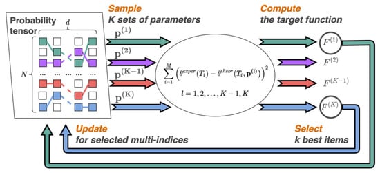
Figure 1. Schematic of PROTES algorithm application.

The PROTES algorithm is executed iteratively:

• Initialization. A discrete probability distribution p over the d-dimensional parameter space is initialized randomly, favoring uniform exploration (i.e., for initial queries, candidates for the optimum will be generated randomly from a distribution close to uniform). The efficiency in high dimensions stems from the compact representation of the discrete array (tensor) p in a structured low-rank TT-format [30], which leads to the fact that the number of parameters in the tensor representation depends linearly on the dimension d of the optimization problem.
• Sampling. At each iteration, K random sets of parameters $p^{\left(l\right)}=\left(p_1^{\left(l\right)},p_2^{\left(l\right)},\dots ,p_d^{\left(l\right)}\right)$ for l = 1, 2, …, K are sampled from the tensor p with a probability proportional to its corresponding values. Note that at the first iteration this will correspond to sampling from a random distribution, and at subsequent iterations the adjusted distribution function will be taken into account. Due to the use of the TT-format, sampling is carried out efficiently with linear complexity in terms of dimensionality.
• Computation. The forward model is solved for each set of parameters l = 1, 2, …, K, and the objective function values F (quantifying mismatch with experiment) are computed.
• Selection and Update. The k samples with the lowest values of F (i.e., best fit to the data) are identified, then the distribution p is updated to increase the probability of sampling these top-k candidates and their neighbors in subsequent iterations. This update is performed efficiently using k_gd gradient-ascent steps on the log-likelihood of the selected samples, leveraging automatic differentiation according to the machine learning paradigm.
• Termination. The above steps are repeated 2–4 times until a predefined computational budget (maximum number of objective function evaluations) m is reached. As iterations progress, p evolves from a broad distribution into a highly peaked one that is centered near the optimal parameter set, $p^{(\ast )}$, and in this case, the approximate value of the optimal parameters will be among the sampled sets during the optimizer iterations.

Computer code, combining PROTES with calculations of objective function, has been developed based on the above algorithm. The following PROTES parameters were used: K = 20, m = 1000, and k = 5.

The PROTES hyperparameters were selected to balance exploratory searches with the computational cost of each function evaluation (one evaluation requires a full solution of the direct problem). The batch size K = 20 and the number of best samples k = 5 lie within the range of standard values recommended in the method’s literature [29] for efficient sampling and updating. The total budget was set to m = 1000 evaluations, which provided a tractable runtime and proved sufficient for convergence to a solution with satisfactory agreement to experiment, demonstrating a dramatic reduction in time compared to manual fitting.

As mentioned earlier, evaluating the objective function F (Equation (11)) requires solving the entire coupled sets of equations twice: once in the reference state (${\tilde{n}}_{{\mathrm{H}}_2}=0$) and once in the sensing state (${\tilde{n}}_{{\mathrm{H}}_2}\ne 0$). This is an inherent requirement of the physical model, as the sensor effect θ is defined as the ratio of electron concentrations in these two distinct chemical environments (Equation (1)). A single evaluation of F on our test workstation (Intel Xeon CPU, 32 GB RAM; Intel Corporation, Santa Clara, CA, USA) takes approximately 20–25 s. This time is dominated by the iterative procedure to find the compatible parameter a (Section 3), which itself requires multiple calls to the BVP solver for each of the two gas states. Therefore, the total cost for one objective function evaluation is roughly double that of solving the system for a single gas state.

While further optimizations (e.g., using a faster root-finding method like Brent’s, or GPU acceleration for the BVP) are possible, the current implementation, leveraging algorithmic robustness and built-in parallelization of PROTES, strikes a good balance between speed, reliability, and code complexity for the problem at hand. The 4–6 h runtime for a full optimization (as discussed in our response to the previous comment) is considered highly efficient compared to the days required for manual fitting.

Certainly, parallelization of the algorithm of the solution of the direct problem would cut the solution time considerably. This is not only due to the necessity to solve the direct problem twice, but in relation to the fact that the objective function is calculated at several different values of temperature.

Parallelization has not been performed in the present study and is left for future investigations.

5. Comparison of Calculated and Experimental Results

Indium oxide was obtained by hydrothermal synthesis, with the average particle size being about 23.5 nm. According to TEM (Transmission Electron Microscopy) data, indium oxide particles of rhombohedral structure have essentially a spherical form and are homogeneous in size.

In order for the sensor response to hydrogen to be determined, synthesized indium oxide was transformed into a metal oxide film. To achieve this, powder was rubbed with distilled water. The suspension, obtained as a result of this process, was placed onto polycor plates equipped with platinum heaters and contacts for reading electrophysical parameters. The plate covered by suspension was gradually heated up to the temperature of 770 K and kept until the resistance of the obtained metal oxide film achieved a constant value.

Measurements of H₂-detecting sensor responses of synthesized films were performed in a special set of experiments within a temperature range from 693 K to 793 K. Temperature was maintained within the accuracy of 1 °C. A chip with an applied sensitive layer was placed within the chamber, with a volume of about 1 cm³. A tested hydrogen–air mixture, containing 1100 ppm H₂ was pumped through the chamber with a flow rate of 20 mL/min. Sensor resistance variation was captured using Digital Multimeter Keysight (Keysight Technologies, Inc., Santa Rosa, CA, USA) and recorded by computer. Specialized software delivered the kinetic curve of resistance variation. Based on the data sensor response θ = R_i/R_g, where R_i is initial (prior to mixture injection) and R_g is minimal (achieved after injection), the value of sensor resistance was determined.

Figure 2 presents the results of the experimental data post-processing in the range from 693 K to 793 K using PROTES. The post-processing provides the following values of the physical parameters:

$$\alpha =1.988;{ \epsilon }_{{\mathrm{O}}_2}^{ads}=7.89\times {10}^{-2};B=8.62\times {10}^{-6};A=1.058\times {10}^2;{\epsilon }_{{\mathrm{H}}_2\mathrm{O}} =8.6\times {10}^{-3}$$

(12)

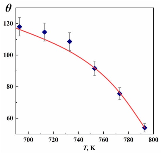
Figure 2. The temperature dependence of In₂O₃ sensor response to hydrogen with a concentration of 1000 ppm. The points are the experimental data, and the curve is the result of fitting procedure using PROTES.

Figure 2 demonstrates that for the obtained parameters (12), the computed curve qualitatively approaches the experimental one; quantitatively, its deviation from the experimental curve does not exceed 5%. This quantitative measure of the deviation is obtained as the NRMSE (Normalized Root Mean Square Error) between the calculated and experimental values over the whole range of the temperatures considered. The exact value calculated by the NRMSE formula is 3.5%. Recall that each invocation of objective function includes the solution of the BVP (6)–(10), enforcement of the condition of electrical neutrality, as well as adjustment of the parameter a. Improved accuracy of approximation may be achieved by significantly increasing the parameter m used by PROTES. In this case, adjustment time increases significantly.

Apart from the comparison of computed and experimental data presented in Figure 2, the gradient-free optimization method PROTES allows the data required for the reconstruction of electron distributions at different locations within nanoparticle, e.g., along its radius (Figure 3), to be obtained.

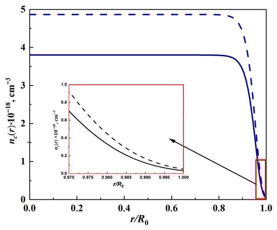
Figure 3. Radial dependence of the conduction electron density n_c(r). Solid curve corresponds to T = 693 K, dashed curve to T = 793 K. The nanoparticle radius R₀ is equal to 37 nm.

For example, it is easy to see that distribution of conduction electrons within the interval 0 ≤ r/R₀ < 0.85 does not change, while their concentration starts to drop upon approaching the border (Figure 3). This results from the possibility of electrons escaping from the volume to the surface of the nanoparticle, where they are captured by adsorbed oxygen atoms. The lack of electrons in the layer adjacent to the surface results in the emergence of an internal electrical field within the nanoparticle. This field repulses free electrons back to the center of the nanoparticle [14,16]. Note that the distribution of conductive electrons within the nanoparticle is a function of temperature, the radius of the nanoparticle, and the relation between the energies of donor levels, the bottom of the conduction band and the binding of electrons with adsorbed oxygen atoms.

6. Conclusions

The present paper demonstrates, using capabilities of methods of machine learning and artificial intelligence for solutions of inverse mathematical problems, emerging methods in the modeling of various physicochemical processes. The problem is considered using an example of sensor effect for detectors based on semiconductor nanoparticles. Steady-state case is studied, where both electron and adsorption (resulting from exchange of electrons between adsorbed oxygen atoms and body of nanoparticle) equilibriums are established. In the state of such equilibriums, reactions involving oxygen and hydrogen proceed at the surface of the nanoparticle. Coupled sets of kinetic equations, describing processes at the surface of nanoparticle, and Poisson’s equation describing electron distribution along its radius, are solved. The presence of the concentration of conductive electrons in the vicinity of the surface of the nanoparticle, in all the above-mentioned equations, significantly complicates the problem. This concentration is considered, in the process of the solution of the coupled set of equations, as a free parameter which needs to be found as part of the solution. Differential equations are compatible with each other at the correct value of such a parameter.

The other mathematical novelty of the paper consists of the application of modern methods of gradient-free optimization and machine learning for carrying out the fitting procedure. A novel algorithm and methodology for calculating physical parameters as well as a solution of the equations using the modern gradient-free optimization method PROTES, which allows for the efficient solution of the inverse problem of parameter search in automatic mode, have been developed. Original computer code has been developed based on the proposed algorithm. Comparison between computed and experimental data has been performed using hydrogen sensitivity of the In₂O₃ oxide sensor. Good agreement between the theoretical and experimental data is evidenced by the NRMSE value of 3.5%.

In future, upon studying more complicated binary nanosystems, the parallelization of the algorithm for solutions of direct problems will be carried out. In addition, the sets of kinetic equations will be expanded to include all possible reactions of gases with the surface of the nanoparticle. The two above modifications would enhance efficiency and accuracy of the application of a developed methodology for the determination of parameters of the inverse problem. It should be noted that the values of the fitted parameters must retain physical significance, when taking into account the available experimental data.

References

- Bandas, C.; Orha, C.; Nicolaescu, M.; Morariu, M.-I.; Lăzău, C. 2D and 3D Nanostructured Metal Oxide Composites as Promising Materials for Electrochemical Energy Storage Techniques: Synthesis Methods and Properties. Int. J. Mol. Sci. 2024, 25, 12521. [Google Scholar] [CrossRef] [PubMed]
- Hajra, K.; Maity, D.; Saha, S. Recent Advancements of Metal Oxide Nanoparticles and their Potential Applications: A Review. Adv. Mater. Lett. 2024, 15, 2401-1740. [Google Scholar] [CrossRef]
- Kant, K.; Beeram, R.; Cao, Y.; Dos Santos, P.S.S.; González-Cabaleiro, L.; García-Lojo, D.; Guo, H.; Joung, Y.; Kothadiya, S.; Lafuente, M.; et al. Plasmonic Nanoparticle Sensors: Current Progress, Challenges, and Future Prospects. Nanoscale Horiz. 2024, 9, 2085–2166. [Google Scholar] [CrossRef] [PubMed]
- Chaabane, L.; Trendafilova, I. Plasmonic Nanostructures for Enhanced Photocatalytic Overall Water Splitting. iScience 2025, 28, 112799. [Google Scholar] [CrossRef]
- Kong, T.; Liao, A.; Xu, Y.; Qiao, X.; Zhang, H.; Zhang, L.; Zhang, C. Recent Advances and Mechanism of Plasmonic Metal-semiconductor Photocatalysis. RSC Adv. 2024, 14, 17041–17050. [Google Scholar] [CrossRef]
- Kumar, A.; Choudhary, P.; Kumar, A.; Camargo, P.H.C.; Krishnan, V. Recent Advances in Plasmonic Photocatalysis Based on TiO2 and Noble Metal Nanoparticles for Energy Conversion. Environ. Remediat. Org. Synth. Small 2022, 18, e2101638. [Google Scholar] [CrossRef]
- Ruoqi, A.; Chui, K.K.; Chen, Y.; Wang, J. Transformation of Plasmonic MoO3-x Nanoparticles into Dielectric MoS2 Nanoparticles. J. Phys. Chem. C 2025, 129, 4126–4133. [Google Scholar] [CrossRef]
- Jia, Y.; Yang, C.; Chen, X.; Xue, W.; Hutchins-Crawford, H.J.; Yu, Q.; Topham, P.D.; Wang, L. A Review on Electrospun Magnetic Nanomaterials: Methods, Properties and Applications. J. Mater. Chem. C 2021, 9, 9042–9082. [Google Scholar] [CrossRef]
- Batlle, X.; Moya, C.; Escoda-Torroella, M.; Iglesias, Ò.; Rodríguez, A.F.; Labarta, A. Magnetic Nanoparticles: From the Nanostructure to the Physical Properties. J. Magn. Magn. Mater. 2022, 543, 168594. [Google Scholar] [CrossRef]
- Zhang, C.; Liu, Y.; Wang, C.; Xu, J.; Bai, Y.-L. In2O3 Decorated Co32 Cluster for High Performance H2S MEMS Sensors. Inorg. Chem. Commun. 2023, 157, 111256. [Google Scholar] [CrossRef]
- Dong, Z.; Hu, Q.; Liu, H.; Wu, Y.; Ma, Z.; Fan, Y.; Li, R.; Xu, J.; Wang, X. 3D Flower-like Ni Doped CeO2 Based Gas Sensor for H2S Detection and its Sensitive Mechanism. Sens. Actuators B Chem. 2022, 357, 131227. [Google Scholar] [CrossRef]
- Wolkenstein, T. Electronic Processes on Semiconductor Surfaces During Chemisorption; Springer: Boston, MA, USA, 1991. [Google Scholar] [CrossRef]
- Kozhushner, M.A.; Trakhtenberg, L.I.; Bodneva, V.L.; Belysheva, T.V.; Landerville, A.C.; Oleynik, I.I. Effect of Temperature and Nanoparticle Size on Sensor Properties of Nanostructured Tin Dioxide Films. J. Phys. Chem. C 2014, 118, 11440–11444. [Google Scholar] [CrossRef]
- Kozhushner, M.A.; Lidskii, B.V.; Oleynik, I.I.; Posvyanskii, V.S.; Trakhtenberg, L.I. Inhomogeneous Charge Distribution in Semiconductor Nanoparticles. J. Phys. Chem. C 2015, 119, 16286–16292. [Google Scholar] [CrossRef]
- Bodneva, V.L.; Ilegbusi, O.J.; Kozhushner, M.A.; Kurmangaleev, K.S.; Posvyanskii, V.S.; Trakhtenberg, L.I. Modeling of Sensor Properties for Reducing Gases and Charge Distribution in Nanostructured Oxides: A Comparison of Theory with Experimental Data. Sens. Actuators B 2019, 287, 218–224. [Google Scholar] [CrossRef]
- Kurmangaleev, K.S.; Ikim, M.I.; Bodneva, V.L.; Posvyanskii, V.S.; Ilegbusi, O.J.; Trakhtenberg, L.I. Sensor Response and Electron Distribution in the Systems of In2O3 Nanoparticles Decorated with CeO2 Nanoclusters. Sens. Actuators B Chem. 2023, 396, 134585. [Google Scholar] [CrossRef]
- Marikutsa, A.; Rumyantseva, M.; Konstantinova, E.A.; Gaskov, A. The Key Role of Active Sites in the Development of Selective Metal Oxide Sensor Materials. Sensors 2021, 21, 2554. [Google Scholar] [CrossRef]
- Yamazoe, N.; Shimanoe, K. Basic Approach to the Transducer Function of Oxide Semiconductor Gas Sensors. Sens. Actuators B Chem. 2011, 160, 1352–1362. [Google Scholar] [CrossRef]
- Morrison, S.R. The Chemical Physics of Surfaces, 2nd ed.; Springer: New York, NY, USA, 1990; 438p. [Google Scholar]
- Suematsu, K.; Ma, N.; Watanabe, K.; Yuasa, M.; Kida, T.; Shimanoe, K. Effect of Humid Aging on the Oxygen Adsorption in SnO2 Gas Sensors. Sensors 2018, 18, 254. [Google Scholar] [CrossRef]
- Ciftyurek, E.; Li, Z.; Schierbaum, K. Adsorbed Oxygen Ions and Oxygen Vacancies: Their Concentration and Distribution in Metal Oxide Chemical Sensors and Influencing Role in Sensitivity and Sensing Mechanisms. Sensors 2023, 23, 29. [Google Scholar] [CrossRef]
- Li, J.; Si, W.; Shi, L.; Gao, R.; Li, Q.; An, W.; Zhao, Z.; Zhang, L.; Bai, N.; Zou, X.; et al. Essential Role of Lattice Oxygen in Hydrogen Sensing Reaction. Nat. Commun. 2024, 15, 2998. [Google Scholar] [CrossRef]
- Morazzoni, M.F.; Ruffo, R.; Scotti, R. Using the Electron Spin Resonance to Detect the Functional Centers in Materials for Sensor Devices. Ionics 2021, 27, 1839–1851. [Google Scholar] [CrossRef]
- Puzzovio, D.; Carotta, M.C.; Cervi, A.; El Hachimi, A.; Joly, J.P.; Gaillard, F.; Guidi, V. TPD and ITPD Study of Materials used as Chemoresistive Gas Sensors. Solid State Ion. 2009, 180, 1545–1552. [Google Scholar] [CrossRef]
- Hao, Z.; Fen, L.; Lu, G.Q.; Liu, J.; An, L.; Wang, H. In Situ Electron Paramagnetic Resonance (EPR) Study of Surface Oxygen Species on Au/ZnO Catalyst for Low-temperature Carbon Monoxide Oxidation. Appl. Catal. A Gen. 2001, 213, 173–177. [Google Scholar] [CrossRef]
- Barsan, N.; Weimar, U. Conduction Model of Metal Oxide Gas Sensors. J. Electroceram. 2001, 7, 143–167. [Google Scholar] [CrossRef]
- Degler, D.; Wicker, S.; Weimar, U.; Barsan, N. Identifying the Active Oxygen Species in SnO2-based Gas Sensing Materials: An Operando IR Spectrsocopy Study. J. Phys. Chem. C. 2015, 119, 11792–11799. [Google Scholar] [CrossRef]
- Gurlo, A. Interplay between O2 and SnO2: Oxygen Ionosorption and Spectroscopicevidence for Adsorbed Oxygen. Chemphyschem 2006, 7, 2041–2052. [Google Scholar] [CrossRef]
- Batsheva, A.; Chertkov, A.; Ryzhakov, G.; Oseledets, I. PROTES: Probabilistic Optimization with Tensor Sampling. Adv. Neural Inf. Process. Syst. 2023, 36, 808–823. [Google Scholar]
- Oseledets, I.V. Tensor-train Decomposition. SIAM J. Sci. Comput. 2011, 33, 2295–2317. [Google Scholar] [CrossRef]
- Sozykin, K.; Chertkov, A.; Schutski, R.; Phan, A.; Cichocki, A.; Oseledets, I. TTOpt: A Maximum Volume Quantized Tensor train-based Optimization and its Application to Reinforcement Learning. Adv. Neural Inf. Process. Syst. 2022, 35, 26052–26065. [Google Scholar]
- Pines, D. Elementary Excitations in Solids; W.A. Benjamin: New York, NY, USA, 1963. [Google Scholar]
- Landau, L.D.; Lifshitz, E.M. Statistical Physics; Elsevier Science: Amsterdam, The Netherlands, 1980; Volume 5. [Google Scholar]
- Novozhilov, V.B.; Bodneva, V.L.; Kurmangaleev, K.S.; Lidskii, B.V.; Posvyanskii, V.S.; Trakhtenberg, L.I. Modeling of the Electronic Structure of Semiconductor Nanoparticles. Mathematics 2023, 11, 2214. [Google Scholar] [CrossRef]
- Rakhuba, M.V.; Oseledets, I.V. Fast Multidimensional Convolution in Low-rank Tensor Formats via Cross Approximation. SIAM J. Sci. Comput. 2015, 37, A565–A582. [Google Scholar] [CrossRef][Green Version]
- Liu, D.; Yang, L.T.; Wang, P.; Zhao, R.; Zhang, Q. TT-TSVD: A multi-modal Tensor Train Decomposition with its Application in Convolutional Neural Networks for smart Healthcare. ACM Trans. Multimed. Comput. Commun. Appl. 2022, 18, 1–17. [Google Scholar] [CrossRef]
- Soley, M.B.; Bergold, P.; Gorodetsky, A.A.; Batista, V.S. Functional Tensor-train Chebyshev Method for Multidimensional Quantum Dynamics Simulations. J. Chem. Theory Comput. 2021, 18, 25–36. [Google Scholar] [CrossRef]
- Núñez Fernández, Y.; Jeannin, M.; Dumitrescu, P.T.; Kloss, T.; Kaye, J.; Parcollet, O.; Waintal, X. Learning Feynman Diagrams with Tensor Trains. Phys. Rev. X 2022, 12, 041018. [Google Scholar] [CrossRef]
- Dolgov, S.; Khoromskij, B.N.; Litvinenko, A.; Matthies, H.G. Polynomial Chaos Expansion of Random Coefficients and the Solution of Stochastic Partial Differential Equations in the Tensor Train Format. SIAM/ASA J. Uncertain. Quantif. 2015, 3, 1109–1135. [Google Scholar] [CrossRef]
- Dolgov, S.; Kalise, D.; Saluzzi, L. Data-driven Tensor Train Gradient Cross Approximation for Hamilton–Jacobi–Bellman Equations. SIAM J. Sci. Comput. 2023, 45, A2153–A2184. [Google Scholar] [CrossRef]
- Jin, X.; Tang, J.; Kong, X.; Peng, Y.; Cao, J.; Zhao, Q.; Kong, W. CTNN: A Convolutional Tensor-train Neural Network for Multi-task Brainprint Recognition. IEEE Trans. Neural Syst. Rehabil. Eng. 2020, 29, 103–112. [Google Scholar] [CrossRef]
- Chien, J.T.; Bao, Y.T. Tensor-factorized Neural Networks. IEEE Trans. Neural Netw. Learn. Syst. 2017, 29, 1998–2011. [Google Scholar] [CrossRef]
- Selvanayagam, C.; Duong, P.L.T.; Wilkerson, B.; Raghavan, N. Global Optimization of Surface Warpage for Inverse Design of Ultra-thin Electronic Packages using Tensor Train Decomposition. IEEE Access 2022, 10, 48589–48602. [Google Scholar] [CrossRef]
- Shetty, S.; Lembono, T.; Loew, T.; Calinon, S. Tensor Train for Global Optimization Problems in Robotics. Int. J. Robot. Res. 2024, 43, 811–839. [Google Scholar] [CrossRef]
Disclaimer/Publisher’s Note: The statements, opinions and data contained in all publications are solely those of the individual author(s) and contributor(s) and not of MDPI and/or the editor(s). MDPI and/or the editor(s) disclaim responsibility for any injury to people or property resulting from any ideas, methods, instructions or products referred to in the content. |
© 2025 by the authors. Licensee MDPI, Basel, Switzerland. This article is an open access article distributed under the terms and conditions of the Creative Commons Attribution (CC BY) license (https://creativecommons.org/licenses/by/4.0/).