Numerical Methods for Decorrelation Stretch

Abstract

Decorrelation stretch is an image enhancement technique that emphasizes color differences, which also applicable to multispectral datasets. It transforms an image so that its color plane result is uncorrelated, with assigned variances. The standard algorithm may suffer from numerical instability. Moreover, it is not able to manage degenerate cases, where color planes are linearly dependent. In this paper, we review the theory behind decorrelation stretch and propose some alternative algorithms that resolve the issues of the standard approach.

1. Introduction

Image enhancement is a well-developed topic, whose aim is to modify the appearance of an image in order to simplify the interpretation of the information contained in it. Different methods have been developed, such as linear contrast enhancement, histogram equalization, neural network, or Gaussian stretch, but some image transformation techniques or filtering methods can also be described as enhancement models [1,2,3,4]. Most of these methods try to enhance (stretch) color differences in images, operating on color bands. Some of them work on the channels separately, but, since color planes may be correlated, the stretching should not be independent for each color [5]. Therefore, it is, in general, preferable to work on the three color bands at the same time.

Decorrelation stretch is an image transformation technique used to enhance color differences, which operates on the three channels simultaneously. It aims to remove the inter-channel correlation found in image pixels; hence, the name “decorrelation stretch”.

It is based on Principal Component Analysis (PCA). Starting from a color image, it finds a linear transformation that, under suitable assumptions, moves data in a reference system where the color bands are uncorrelated. Then, the bands are stretched to enhance color differences. The aim is to achieve an output image whose pixels are spread along all possible colors, resulting in an improvement in the intensity and saturation of colors. This model has been largely studied [6,7,8,9], and applied in different fields, e.g., geological studies described in [10,11,12], or archeological applications in [13,14,15,16,17,18,19,20,21,22,23,24], or medical studies in [25,26,27,28].

The method is most effective for images where bands (channels) are highly correlated, e.g., satellite or aerial images where different bands capture very similar information. Even in standard natural-color photographs, the red, green, and blue channels are not independent. Decorrelation stretch reduces this correlation to highlight subtle differences in color. Our work is motivated by the necessity to understand whether there are paintings in rock walls of archeological sites that have been hidden by the passage of time or confused with the presence of moss and vegetation.

While digital color images generally consist of three matrices storing red, green, and blue (RGB) components of each pixel, multispectral images investigate information in specific wavelength ranges, even non-visible ones. They are used in remote sensing for capturing information that the human eye fails to detect, and often include 7–15 spectral bands. A particular situation is that of hyperspectral images, which may involve hundreds of bands.

In some applications, to be able to visualize data as a standard color image, it is common to select in advance three particular frequency bands in a multispectral image, on the basis of physical information on the phenomenon under scrutiny. However, this does not necessarily have to be performed before data processing, as decorrelation stretch, like other image enhancement techniques, does not substantially change if applied to three-plane images or to multispectral ones. Moreover, processing the complete dataset leads to automatically identifying the spectral components which are most relevant in the observation.

In this work, we first resume the decorrelation stretch method and clearly state its statistical properties. In particular, we discuss the degenerate case of linearly dependent color planes, which does not appear to have been discussed in the past. Then, we propose some new algorithms, with the aim of reducing the computational load and increasing accuracy. One of the proposed methods is also able to correctly treat degenerate cases, producing images with decorrelated color channels. Such approaches are compared to an existing implementation of the method, namely, the MATLAB function decorrstretch; in this paper we always refer to version R2024b of MATLAB. Reducing the complexity of the computation is particularly useful when large datasets have to be processed, or when hyperspectral images are considered.

The paper is organized as follows: Section 2 recalls some basic statistical concepts to fix the notation; Section 3 reviews the decorrelation stretching process and its MATLAB implementation decorrstretch; and Section 4 underlines some issues of this implementation and explains how we propose to solve them. Section 5 shows some applications and discusses the results obtained by applying the proposed methods. Lastly, Section 6 contains our final considerations.

2. Statistical Preliminaries

Let y be a random variable with the distribution function $F\left(y\right)$. Its mean value and variance are defined as

$$\begin{array}{cc}\hfill \mu & =E\left[y\right]={\int }_{-\infty }^{\infty }ydF\left(y\right),\hfill \end{array}$$

(1)

$$\begin{array}{cc}\hfill {\sigma }^2& =E\left[{(y-\mu )}^2\right]={\int }_{-\infty }^{\infty }{(y-\mu )}^{2}dF\left(y\right).\hfill \end{array}$$

(2)

Now, let $\mathbf{y}={(y_1,\dots ,y_n)}^T$ be a vector of random variables. If $F(y_i,y_j)$ is the joint distribution of $y_i$ and $y_j$, then the covariance of the two random variables is

$${\sigma }_{i,j}=cov(y_i,y_j)=E\left[(y_i-{\mu }_i)(y_j-{\mu }_j)\right]={\int }_{{\mathbb{R}}^2}(y_i-{\mu }_i)(y_j-{\mu }_j)dF(y_i,y_j).$$

Notice that ${\sigma }_{i,i}={\sigma }_i^2=E\left[{(y_i-{\mu }_i)}^2\right]$. The variables $y_i$ and $y_j$ are said to be uncorrelated if ${\sigma }_{i,j}=0$.

For a vector of random variables, we extend the definition of the operator E to act, componentwise, on its arguments. So, we will write $\mathit{\mu }=E\left[\mathbf{y}\right]\in {\mathbb{R}}^n$, meaning that ${\mu }_i=E\left[y_i\right]$, and define the variance–covariance matrix of $\mathbf{y}$ as

$$\mathcal{V}=\mathcal{V}\left[\mathbf{y}\right]=E\left[(\mathbf{y}-\mathit{\mu }){(\mathbf{y}-\mathit{\mu })}^T\right],$$

so that ${\mathcal{V}}_{i,j}={\sigma }_{i,j}$.

The correlation matrix of $\mathbf{y}$ is obtained by

$$\mathcal{C}=\mathcal{C}\left[\mathbf{y}\right]={\sum }^{-1}\mathcal{V}{\sum }^{-1},$$

(3)

where $\sum =\mathrm{diag}({\sigma }_1,\dots ,{\sigma }_n)$ contains the standard deviations of the components of $\mathbf{y}$. Its diagonal entries are unitary, while the off-diagonal elements are the correlation coefficients for each pair of variables, i.e., ${\mathcal{C}}_{i,j}={\displaystyle \frac{{\sigma }_{i,j}}{{\sigma }_i{\sigma }_j}}$, for $i\ne j$. We will say that a random vector is uncorrelated when each pair of its components is as such. The correlation coefficient is undefined when the variable is constant, as it has zero variance.

The following theorem can be easily proved by applying the linearity of E.

Theorem 1.

Let M be a matrix of dimension $r\times n$ and let $\mathbf{z}=M\mathbf{y}$. If $\mathit{\mu }=E\left[\mathbf{y}\right]$ and $\mathcal{V}=\mathcal{V}\left[\mathbf{y}\right]$, then the mean value and the variance–covariance matrix of the linearly transformed random vector are

$$E\left[\mathbf{z}\right]=M\mathit{\mu }\mathrm{and}\mathcal{V}\left[\mathbf{z}\right]=M\mathcal{V}{M}^T.$$

When a discrete sampling $(y_1,\dots ,y_m)$ of a random variable is available, assuming uniform distribution, the mean value (1) and variance (2) are computed by

$$\mu ={\displaystyle \frac{1}{m}}\sum _{i=1}^m{y}_i,{\sigma }^2={\displaystyle \frac{1}{m-1}}\sum _{i=1}^m{(y_i-\mu )}^2.$$

In the case of a random vector $\mathbf{y}$, we will pack its realizations in a matrix

$$Y=\left[\begin{array}{c}{\mathbf{y}}_1,\dots ,{\mathbf{y}}_m\end{array}\right],$$

and write

$$\mathit{\mu }={\displaystyle \frac{1}{m}}Y\mathbf{u},\mathcal{V}={\displaystyle \frac{1}{m-1}}(Y-\mathit{\mu }{\mathbf{u}}^T){(Y-\mathit{\mu }{\mathbf{u}}^T)}^T,$$

(4)

where $\mathbf{u}={(1,\dots ,1)}^T\in {\mathbb{R}}^m$.

Remark 1.

Statistical independence and linear independence, commonly encountered in numerical linear algebra, are fundamentally different concepts and should not be conflated. First of all, if two variables are statistically independent and possess finite variance, then they are necessarily uncorrelated. However, the converse is not true: uncorrelated variables are not necessarily statistically independent. Nevertheless, uncorrelatedness implies the absence of a linear relationship between the variables, but nonlinear forms of dependence may still be present.

3. Decorrelation Stretch

Decorrelation stretch (DS), starting from a color image, seeks a linear spatial transformation which decorrelates and stretches colors. The process can be described by matrix and vector operations, and can be expressed by a single mathematical transformation that takes, as input, an image and produces the decorrelation-stretched output.

DS [6] is strictly connected to Principal Component Analysis (PCA). The basic PCA procedure leads to the construction of a vector of uncorrelated random variables, starting from a vector of correlated ones, by changing the reference system.

Let $\mathbf{y}$ be a vector of random variables with mean value $\mathit{\mu }$ and variance–covariance (V-C) matrix $\mathcal{V}$. The matrix $\mathcal{V}$ is symmetric and positive semi-definite, so it admits a spectral factorization

$$\mathcal{V}=Q\Lambda Q^T,$$

where $\mathrm{\Lambda }=\mathrm{diag}({\lambda }_1,\dots ,{\lambda }_n)$ contains the eigenvalues ${\lambda }_i\ge 0$ and the columns of the orthogonal matrix $Q=[{\mathbf{q}}_1,\dots ,{\mathbf{q}}_n]$ are the eigenvectors.

Proposition 1.

The components of the transformed vector $\mathbf{z}=Q^T\mathbf{y}$ are uncorrelated.

Proof. 

By Theorem 1 the new vector $\mathbf{z}=Q^T\mathbf{y}$ has mean $E\left[\mathbf{z}\right]=Q^T\mathit{\mu }$ and V-C matrix

$$\mathcal{V}\left[\mathbf{z}\right]=Q^T\mathcal{V}Q=\Lambda ,$$

that is, the components of $\mathbf{z}$ are uncorrelated with variances equal to the eigenvalues of $\mathcal{V}$.    □

Decorrelation stretch allows one to construct a new random vector of uncorrelated components with the desired variances.

Proposition 2.

Under the assumption that ${\lambda }_i\ne 0$, $\forall i=1,\dots ,n$, let us consider the “DS” transformation

$$M={\sum }_{T}Q{\Lambda }^{-{\displaystyle \frac{1}{2}}}{Q}^T,$$

(5)

where

$${\Lambda }^{-{\displaystyle \frac{1}{2}}}=\mathrm{diag}\left({\displaystyle \frac{1}{\sqrt{{\lambda }_1}}},\dots ,{\displaystyle \frac{1}{\sqrt{{\lambda }_n}}}\right)$$

and ${\sum }_T=\mathrm{diag}({\overline{\sigma }}_1,\dots ,{\overline{\sigma }}_n)$, for chosen target variances ${\overline{\sigma }}_i^2$. Then, the components of the transformed vector $\mathbf{z}=M\mathbf{y}$ are uncorrelated with variances ${\overline{\sigma }}_i^2$.

Proof. 

Computing the V-C matrix of $\mathbf{z}=M\mathbf{y}$ by Theorem 1 and using the spectral factorization of $\mathcal{V}$, one obtains

$$\mathcal{V}\left[\mathbf{z}\right]=M\mathcal{V}{M}^T=({\sum }_{T}Q{\Lambda }^{-{\displaystyle \frac{1}{2}}}{Q}^T)(Q\Lambda Q^T)(Q{\Lambda }^{-{\displaystyle \frac{1}{2}}}{Q}^T{\sum }_T)={\sum }_T^2,$$

(6)

that is, the new variables $z_i$ are uncorrelated with variance ${\overline{\sigma }}_i^2$.    □

A similar transformation based on the correlation matrix (3) of $\mathbf{y}$ can be constructed. In this case, one considers its spectral factorization

$$\mathcal{C}=Q\Lambda Q^T.$$

Proposition 3.

Assuming $\mathcal{C}$ is symmetric and positive definite, i.e., ${\lambda }_i>0$, and considering the transformation

$$N={\sum }_{T}Q{\Lambda }^{-{\displaystyle \frac{1}{2}}}{Q}^T{\sum }^{-1},$$

(7)

the V-C matrix of the transformed vector $\mathbf{w}=N\mathbf{y}$ is $\mathcal{V}\left[\mathbf{w}\right]={\sum }_T^2$.

Proof. 

From Theorem 1 and from the definition of correlation matrix (3), using its spectral factorization, one obtains

$$\begin{array}{cc}\hfill \mathcal{V}\left[\mathbf{w}\right]=N\mathcal{V}{N}^T& =({\sum }_{T}Q{\Lambda }^{-{\displaystyle \frac{1}{2}}}{Q}^T{\sum }^{-1})\mathcal{V}({\sum }^{-1}Q{\Lambda }^{-{\displaystyle \frac{1}{2}}}{Q}^T{\sum }_T)\hfill \\ & =({\sum }_{T}Q{\Lambda }^{-{\displaystyle \frac{1}{2}}}{Q}^T)(Q\Lambda Q^T)(Q{\Lambda }^{-{\displaystyle \frac{1}{2}}}{Q}^T{\sum }_T)={\sum }_T^2.\hfill \end{array}$$

   □

This shows that even if the transformed vectors $\mathbf{z}=M\mathbf{y}$ and $\mathbf{w}=N\mathbf{y}$ differ in general, they share important statistical features, as they are both uncorrelated and their V-C matrices coincide.

A dataset is considered an image when it consists of a 3D array $\mathcal{I}$ of size $r\times c\times n$. Monochrome images are characterized by $n=1$; the resulting $r\times c$ matrix contains grayscale intensity information for each pixel. For RGB images, $n=3$ and the layers ${\mathcal{I}}_k={\mathcal{I}}_{(·,·,k)}$, $k=1,2,3$, store intensity information for the red, green, and blue color channels. In multispectral and hyperspectral images, n is larger than 3 and each layer corresponds to a particular electromagnetic frequency band. Other applications may concern datasets that are not directly connected to visible phenomena or to electromagnetic waves, but that can be regarded as “images”.

When images are numerically processed, they are usually “vectorized”, that is, the array $\mathcal{I}$ is converted to a matrix A of size $p\times n$, where $p=rs$ is the number of pixels. Each column $A_k=A_{(·,k)}$ of A is obtained by lexicographically ordering the corresponding kth layer.

In DS, one associates to an image pixel a random vector $\mathbf{y}\in {\mathbb{R}}^n$, whose components represent the corresponding “color” layer information for that pixel. An image contains p realizations of this random vector

$$Y=\left[\begin{array}{c}{\mathbf{y}}_1,\dots ,{\mathbf{y}}_p\end{array}\right]=A^T,$$

(8)

which are usually assumed to be uniformly distributed. This makes it possible to associate to the image a mean vector and a V-C matrix by Formula (4), that is

$$\mathit{\mu }={\displaystyle \frac{1}{p}}{A}^T\mathbf{u},\mathcal{V}={\displaystyle \frac{1}{p-1}}(A^T-\mathit{\mu }{\mathbf{u}}^T){(A^T-\mathit{\mu }{\mathbf{u}}^T)}^T.$$

(9)

At this point, the linear transformation (5) is applied to Y. This rotates the reference system in that of the principal components, i.e., the eigenvectors of $\mathcal{V}$, where the variables are uncorrelated. Here, the variables are scaled to take on unitary variances, and then they are rotated back to the original reference, where they are still uncorrelated. The resulting vectors are stretched so that they assume target variances ${\overline{\sigma }}_i^2$, $i=1,\dots ,n$. Finally, target mean values ${\mathit{\mu }}_T$ can be imposed on the resulting dataset.

The complete transformation is

$$S=MY+({\mathit{\mu }}_T-M\mathit{\mu }){\mathbf{u}}^T=M(Y-\mathit{\mu }{\mathbf{u}}^T)+{\mathit{\mu }}_T{\mathbf{u}}^T,$$

and the final $n\times p$ matrix S, after transposition, is reshaped in a $r\times c\times n$ “image”. By default, one usually sets ${\sum }_T=\sum$ and ${\mathit{\mu }}_T=\mathit{\mu }$. A similar process can be constructed by substituting the correlation matrix $\mathcal{C}$ to the V-C matrix $\mathcal{V}$, and the transformation (7) to (5). The above procedure is implemented in the MATLAB function decorrstretch.

The Special Case of a Singular V-C Matrix

When an eigenvalue of the matrix $\mathcal{V}$ is zero, transformation (5) cannot be constructed, due to the presence of the matrix ${\Lambda }^{-{\displaystyle \frac{1}{2}}}$. Given definition (3), the same happens when the construction is based on the correlation matrix.

Two significant situations in which this feature appears are the following. First of all, if the ith color plane is constant, the variance of the component $y_i$ of the random vector $\mathbf{y}$ is zero, as well as the covariances of the pairs $(y_i,y_j)$ for any $j\ne i$. This means that the ith color plane is completely uncorrelated to the other ones. It might be removed from the dataset before processing, and inserted back after the computation.

Another relevant case is when a color plane is a linear combination of other planes. In this case, that layer is intrinsically correlated to the ones that generated it, and DS cannot diagonalize the V-C matrix. We remark that if a group of layers is linearly dependent, it is possible to identify the layers to be removed by applying the modified Gram–Schmidt method [29] to the columns of A. Indeed, a breakdown at the kth step of the algorithm indicates that the kth vector is a linear combination of the previous ones. In this case, the vector can simply be removed before executing the next step.

The case of a singular V-C matrix, that is, a constant or perfectly linearly dependent color channel, is rather unlikely to be encountered in field photography or in remote sensing. However, it might happen in applications where the observed target is illuminated by light of a specific color, which happens in monochrome microscopy. Furthermore, a mathematical model and its software implementation should be robust with respect to input data, so the problem must be addressed.

In the following, we give a mathematical justification of the failure of DS in the presence of zero eigenvalues. Formally, it is possible to proceed even in this situation by substituting ${\Lambda }^{-{\displaystyle \frac{1}{2}}}$ with the square root of the pseudoinverse $\sqrt{{\Lambda }^{†}}$. The pseudoinverse matrix can be defined in terms of the SVD factorization (see [29]), but in the case of a diagonal matrix, its construction is immediate. Indeed, if $\Lambda =\mathrm{diag}({\lambda }_1,\dots ,{\lambda }_n)$, then the pseudoinverse ${\Lambda }^{†}$ is a diagonal matrix with diagonal elements

$${\left({\Lambda }^{†}\right)}_{i,i}=\left\{\begin{array}{cc}{\lambda }_i^{-1},\hfill & {\lambda }_i\ne 0,\hfill \\ 0,\hfill & {\lambda }_i=0.\hfill \end{array}\right.$$

If this happens, Equation (6) becomes

$$\mathcal{V}\left[\mathbf{z}\right]=M\mathcal{V}{M}^T={\sum }_{T}Q\sqrt{{\Lambda }^{†}}\Lambda \sqrt{{\Lambda }^{†}}{Q}^T{\sum }_T={\sum }_{T}Q\mathcal{J}{Q}^T{\sum }_T,$$

(10)

where the matrix $\mathcal{J}=\sqrt{{\Lambda }^{†}}\Lambda \sqrt{{\Lambda }^{†}}$ is diagonal with diagonal elements

$${\mathcal{J}}_{i,i}=\left\{\begin{array}{cc}1\hfill & {\lambda }_i\ne 0,\hfill \\ 0,\hfill & {\lambda }_i=0.\hfill \end{array}\right.$$

Due to this fact, the matrix $Q\mathcal{J}{Q}^T$ appearing in (10) is nondiagonal. Indeed, it is the linear transformation that orthogonally projects a vector in the space spanned by the eigenvectors of $\mathcal{V}$ corresponding to nonzero eigenvalues. As a consequence, the components of the resulting random vector $\mathbf{z}$ are not uncorrelated, and DS cannot be successfully applied.

The MATLAB function decorrstretch implements the above procedure based on the pseudoinverse of $\Lambda$. Additionally, it considers the transformation

$$\tilde{\mathbf{z}}=\tilde{M}\mathbf{y}=KM\mathbf{y},$$

where the diagonal matrix K is given by

$$K={\sum }_T{\left(\mathrm{diag}{\left(M\mathcal{V}{M}^T\right)}^{†}\right)}^{{\displaystyle \frac{1}{2}}}.$$

It is straightforward to verify that if the V-C matrix $\mathcal{V}$ is nonsingular, K is the identity matrix, so that in this case the modified algorithm does not change the result of DS.

When at least one of the eigenvalues of $\mathcal{V}$ is zero, K introduces a scaling factor in the components of $\tilde{\mathbf{z}}$, so that its variances are the target values ${\overline{\sigma }}_i^2$. In any case, this transformation does not change the fact that the components are correlated, so DS has practically no effect on the enhancement of the image. For this reason, we will not consider this transformation in our computation. Our decision is supported by the fact that the presence of a linearly dependent color layer is not likely in experimental data. Moreover, in case this happens, we consider it preferable to remove the dependent layer from the image, as it does not contain significant information, and process the reduced dataset. If one chooses to process the correlation matrix $\mathcal{C}$ and applies the transformation (7), all the above considerations are still valid.

In the following, we will describe an algorithm for DS that can detect a degenerate case and automatically reduce the dataset to produce an output image with uncorrelated color channels.

4. New Numerical Approaches to DS

The algorithm outlined in Section 3 has various numerical flaws. Firstly, it stands on the computation of the matrix $C=A^{T}A$. It is known that such operation is heavily affected by underflows and overflows, which may cause loss of information, and is not backward stable ([29], Section 2.1.2). This last statement means that for the computed matrix $\overline{C}$, which is influenced by rounding errors, it is not possible to prove that there exists a small perturbation matrix E, such that $\overline{C}={(A+E)}^T(A+E)$.

Further, we showed in Section 3 that in the case of a singular V-C matrix, the approach used in the MATLAB function decorrstretch does not produce uncorrelated color components for an image, and is of little use. Finally, the above procedure does not automatically deal with linearly dependent color planes and, to produce uncorrelated data, forces the user to check for the presence of numerically zero eigenvalues of the V-C matrix, remove the corresponding components from the data, and rerun the DS algorithm.

To deal with these problems, we propose to perform the computation using the singular value decomposition (SVD) of A, instead of computing $A^{T}A$. A clever use of a QR factorization, before computing the SVD, leads to a modified algorithm requiring less computing time and a smaller storage space, but also gives the opportunity to efficiently treat the case of a singular V-C matrix, producing uncorrelated stretched color planes. If accuracy is not an issue, but speed of processing is, we propose to apply a randomized approach to any of the previous methods to reduce their runtime.

The algorithms introduced in this paper produce results equivalent to those obtained when DS is applied to the V-C matrix. They are not suitable to be applied to the correlation matrix. In any case, we remark that the resulting random vectors are statistically equivalent because, as already noted in Proposition 3, they share the same V-C matrix. Moreover, according to our experience, the results produced by the two approaches are visually indistinguishable.

4.1. SVD-Based Decorrelation Stretch

We consider the compact SVD factorization of ${(Y-\mathit{\mu }{\mathbf{u}}^T)}^T=A-\mathbf{u}{\mathit{\mu }}^T$ (see Equations (8) and (9))

$$A-\mathbf{u}{\mathit{\mu }}^T=UD{V}^T,D=\mathrm{diag}(d_1,\dots ,d_n),$$

(11)

where $U\in {\mathbb{R}}^{p\times n}$ and $V\in {\mathbb{R}}^{n\times n}$ have orthonormal columns, called left and right singular vectors, and $d_i\ge 0$ are the singular values. The number of nonzero singular values equals the rank of the matrix, and of $\mathcal{V}$.

While V and D are “small” matrices, of size coincident with the number of color planes in the image, U has the same size as A, so it may be quite large. In any case, the matrix U is not needed in the process. Indeed, the right singular vectors, i.e., the columns of V, are the eigenvectors of $\mathcal{V}$, and its eigenvalues coincide with $d_i^2/(p-1)$, for $i=1,\dots ,n$. This can be easily verified by substituting the SVD (11) in the computation of the V-C matrix

$$\mathcal{V}={\displaystyle \frac{1}{p-1}}\left(Y-\mathit{\mu }{\mathbf{u}}^T\right){\left(Y-\mathit{\mu }{\mathbf{u}}^T\right)}^T={\displaystyle \frac{1}{p-1}}V{D}^{T}D{V}^T.$$

This implies that transformation (5) based on the SVD can be written as

$$M=\sqrt{p-1}{\sum }_{T}V{D}^{-1}{V}^T.$$

(12)

4.2. Q-Less QR + SVD

Even if the matrix U in (11) is not required for DS, the SVD algorithm creates it. To reduce time and storage space, one can consider an approach based on the application of the compact QR decomposition

$${\left(Y-\mu {\mathbf{u}}^T\right)}^T=QR,$$

(13)

where Q is a matrix with orthogonal columns of size $p\times n$ and R is a square upper triangular matrix of size n. The factorization algorithm allows one to avoid the allocation and computation of the matrix Q. The triangularization is performed by applying n fast Householder transformations to the starting matrix [30]. This feature is implemented in the qr function of MATLAB and is called Q-less QR factorization.

Once (13) is obtained, the SVD decomposition $R=\tilde{U}D{V}^T$ of the resulting triangular matrix is computed. Then, the SVD of the initial matrix is given by

$${\left(Y-\mathit{\mu }{\mathbf{u}}^T\right)}^T=Q\tilde{U}D{V}^T=UD{V}^T,$$

where the matrix $U=Q\tilde{U}$ is not explicitly computed, since it is not needed in (12). This makes it possible to compute transformation M by a faster algorithm and save the allocation of a $p\times n$ matrix, while preserving the stability of the procedure.

Another advantage of this approach is that it allows the direct treatment of a rank-deficient V-C matrix. Indeed, for a fixed tolerance $\tau$, let

$$\mathcal{S}=\left\{i:|r_{i.i}|<\tau \right\}$$

be the set of indices corresponding to “zero” diagonal elements in R. Then, the columns of A with index in $\mathcal{S}$ are either constant or linear combinations of other columns. This is a consequence of the fact that a QR factorization is an orthonormalization process for the columns of A.

If the set $\mathcal{S}$ is nonempty, the corresponding columns of A are removed, as well as the rows and columns of R with index in $\mathcal{S}$. At this point, the transformation (12) is constructed and applied to the linearly independent columns of A. Finally, the columns of A with index in $\mathcal{S}$ are reintroduced in the dataset as zero columns. This produces uncorrelated color planes, differently from what happens using the procedure described in Section 3.

If, for some reason, the V-C matrix of the original dataset is needed, it can be computed with reduced complexity by

$$\mathcal{V}={\displaystyle \frac{1}{p-1}}{R}^{T}R.$$

In particular, the variances are given by

$${\sigma }_i^2={\displaystyle \frac{1}{p-1}}\sum _{j=1}^i{r}_{j,i}^2,i=1,\dots ,n.$$

4.3. A Randomized Approach

When large datasets must be processed and computing speed is important, one may be prone to renouncing some accuracy to obtain faster results.

A simple solution is to consider a randomly constructed sub-image of the original one. This can be easily performed by extracting a random subsampling of the rows of A, using this reduced dataset to compute the DS linear transformation, and then applying it to the initial image. This idea can be applied to any of the algorithms described in this paper.

In our tests, we fixed a percentage $\varphi \in (0,1]$ and extracted a subsampling of $\lfloor \varphi p\rfloor$ rows of A, where $\lfloor z\rfloor$ denotes the integer part of z. As expected, the error between the computation performed with the full dataset and the reduced one becomes larger as $\varphi$ decreases, but we will show in the numerical experiments that even relatively large errors produce almost imperceptible visual differences.

The numerical methods presented in this paper are outlined in Algorithm 1. It takes as input the image to be processed and the target variances and mean values. The method can be either SVD or QR-SVD. If the parameter $\varphi$ is 1, the standard algorithms are applied. If $\varphi <1$, the randomized methods are applied instead. Computational routines for computing SVD and QR factorizations are contained in any scientific software environment, besides MATLAB, and are available in the LAPACK library https://www.netlib.org/lapack/ (accessed on 8 September 2025), which can be linked to all high level programming languages.

Algorithm 1 Outline of SVD, QR-SVD, and rand-QR-SVD approaches to DS.

Require: image $X\in {\mathbb{R}}^{r\times c\times n}$, method, target variance matrix ${\sum }_T$, target mean vector ${\mathit{\mu }}_T$, percentage $\varphi \in (0,1]$ forthe randomized approach, tolerance $\tau$

Ensure: stretched image X

1: convert image pixel values to double precision

2: reshape image X to a matrix $A\in {\mathbb{R}}^{p\times n}$, where $p=rc$

3: store in vector $\mathit{\mu }$ the mean values of the columns of A

4: $\tilde{A}=A-\mathit{\mu }$

5: if $\varphi <1$then

6:      store in $\sigma$ a random subsampling of $\lfloor \varphi p\rfloor$ rows of A

7:      $\tilde{A}={\tilde{A}}_{\sigma }$ (apply the subsampling to $\tilde{A}$)

8: end if

9: if method = SVD then

10:      compute compact SVD factorization $\tilde{A}=US{Q}^T$

11:      $\Lambda =S/\sqrt{p-1}$

12:      if any ${\Lambda }_{i,i}<\tau$ then

13:          issue an error: the V-C matrix is numerically singular

14:      end if

15:   end if method = QR-SVD

16:      compute R as triangular factor of Q-less QR factorization $\tilde{A}=QR$

17:      construct set $\mathcal{S}=\left\{i:|r_{i.i}|<\tau \right\}$

18:      if $\mathcal{S}$ is not empty then

19:          remove from R and ${\sum }_T$ rows and columns indexed in $\mathcal{S}$

20:          remove from A columns indexed in $\mathcal{S}$

21:          remove from $\mathit{\mu }$ and ${\mathit{\mu }}_T$ components indexed in $\mathcal{S}$

22:      end if

23:      compute compact SVD factorization $R=US{Q}^T$

24:      $\Lambda =S/\sqrt{p-1}$

25: end if

26: $M=Q{\Lambda }^{-1}{Q}^T{\sum }_T$

27: $A=(A-\mu )M+{\mathit{\mu }}_T$

28: reshape matrix $A\in {\mathbb{R}}^{p\times n}$ to an image $X\in {\mathbb{R}}^{r\times c\times n}$

5. Results and Discussion

The numerical experiments were performed on an Intel Core i9-14900KF computer with 128 GB RAM (Intel Corporation, Santa Clara, CA, USA), running Linux Debian 12 and MATLAB R2024b.

Four test images were used in the experiments:

• rand($r,c,n$): A randomly generated image with resolution $r\times c$ and n color planes, for chosen values of r, c, and n, with pixel values uniformly distributed in $[0,1]$;
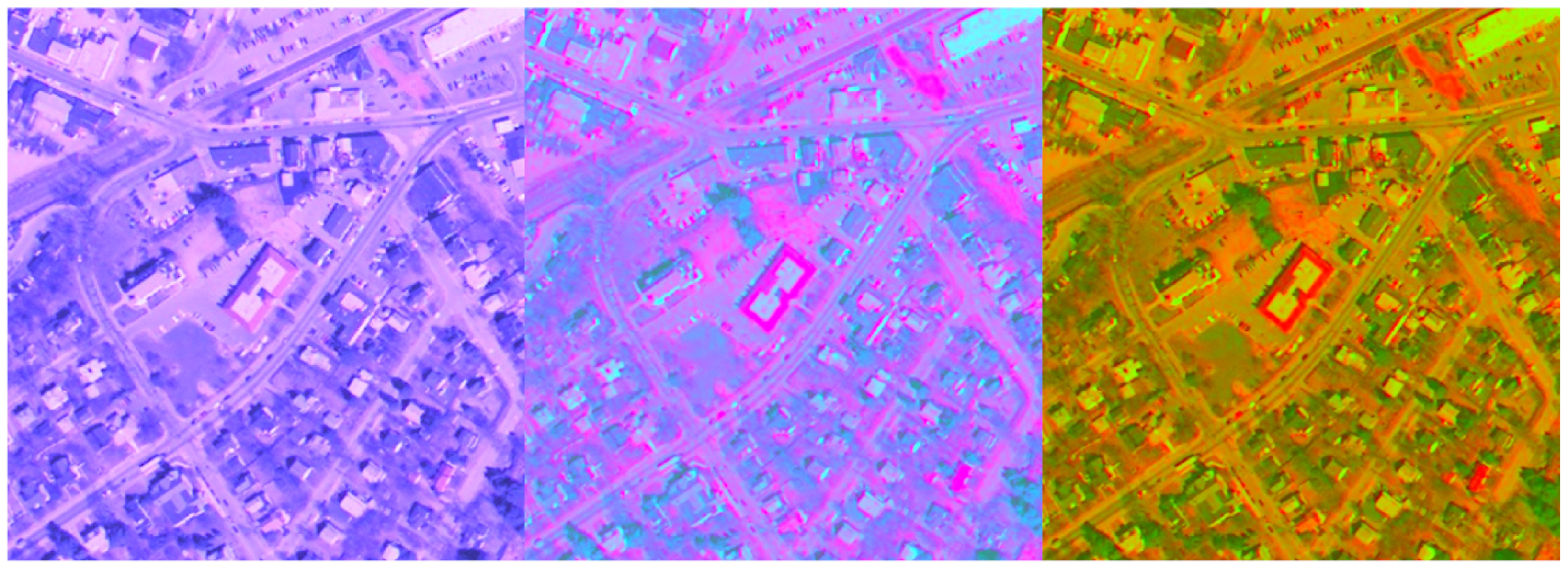
• west: The aerial RGB color image westconcordaerial.png with resolution, $394\times 369$, available in the MATLAB library;
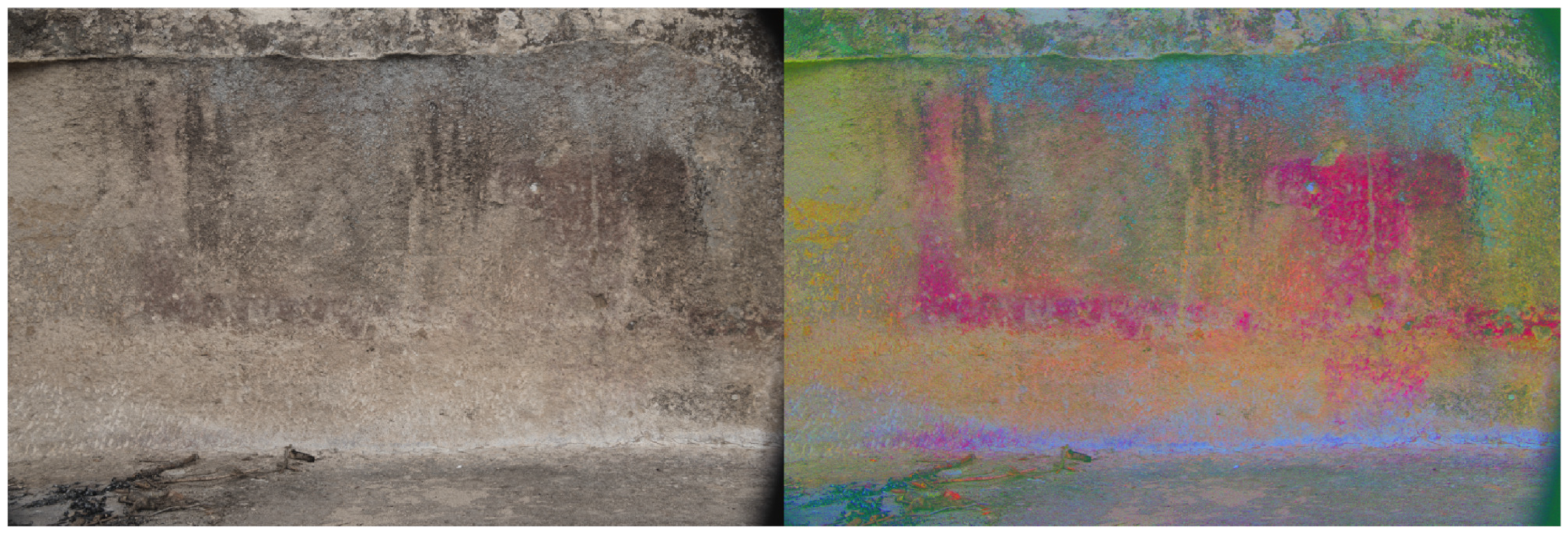
• pimentel: A RGB color image with resolution $4012\times 6016$, taken by the authors at the archeological site Domus de Janas de S’Acqua Salida (Pimentel, Italy); domus de janas (fairy houses) are Neolithic funerary hypogea typical of the Island of Sardinia;
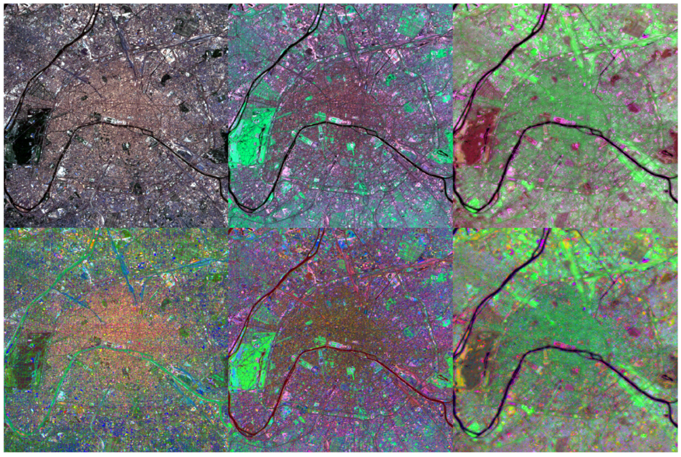
• paris: The multispectral dataset paris.lan containing a Landsat image of Paris with resolution $512\times 512$, available in the MATLAB documentation.

The MATLAB function dextre.m, developed for this work, is available at the web page https://bugs.unica.it/~cana/software (accessed on 8 September 2025), as well as the pimentel image, in CR3 raw format.

The first numerical test concerns the speed of execution. We initially consider random RGB images rand($r,r,3$) for $r=200,400,\dots ,3000$. We apply to each test image the function decorrstretch from MATLAB, the proposed methods of Section 4.1 and Section 4.2, which we denote SVD and QR-SVD, and the randomized approach of Section 4.3 with $\varphi ={10}^{-3}$, labeled as rand-QR-SVD. Each method is applied 10 times and we measure the average execution time. 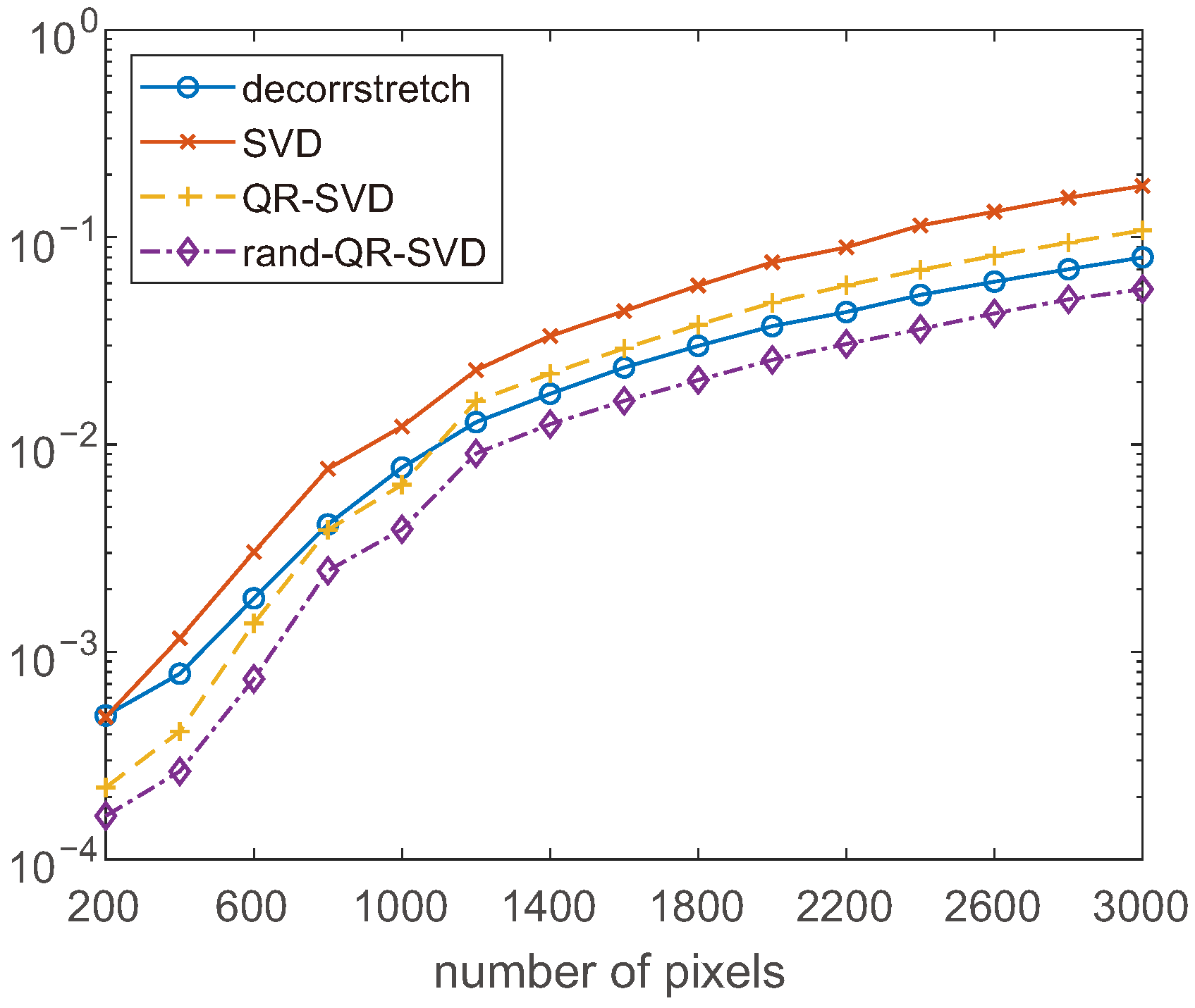Figure 1 reports the measured timings in seconds. The two SVD-based methods are slightly slower than the classical approach: the ratio between their timings and decorrstretch for large r values is about 2 for SVD and 1.3 for QR-SVD. The last method is faster for small sizes. The randomized QR-SVD method is clearly the fastest.

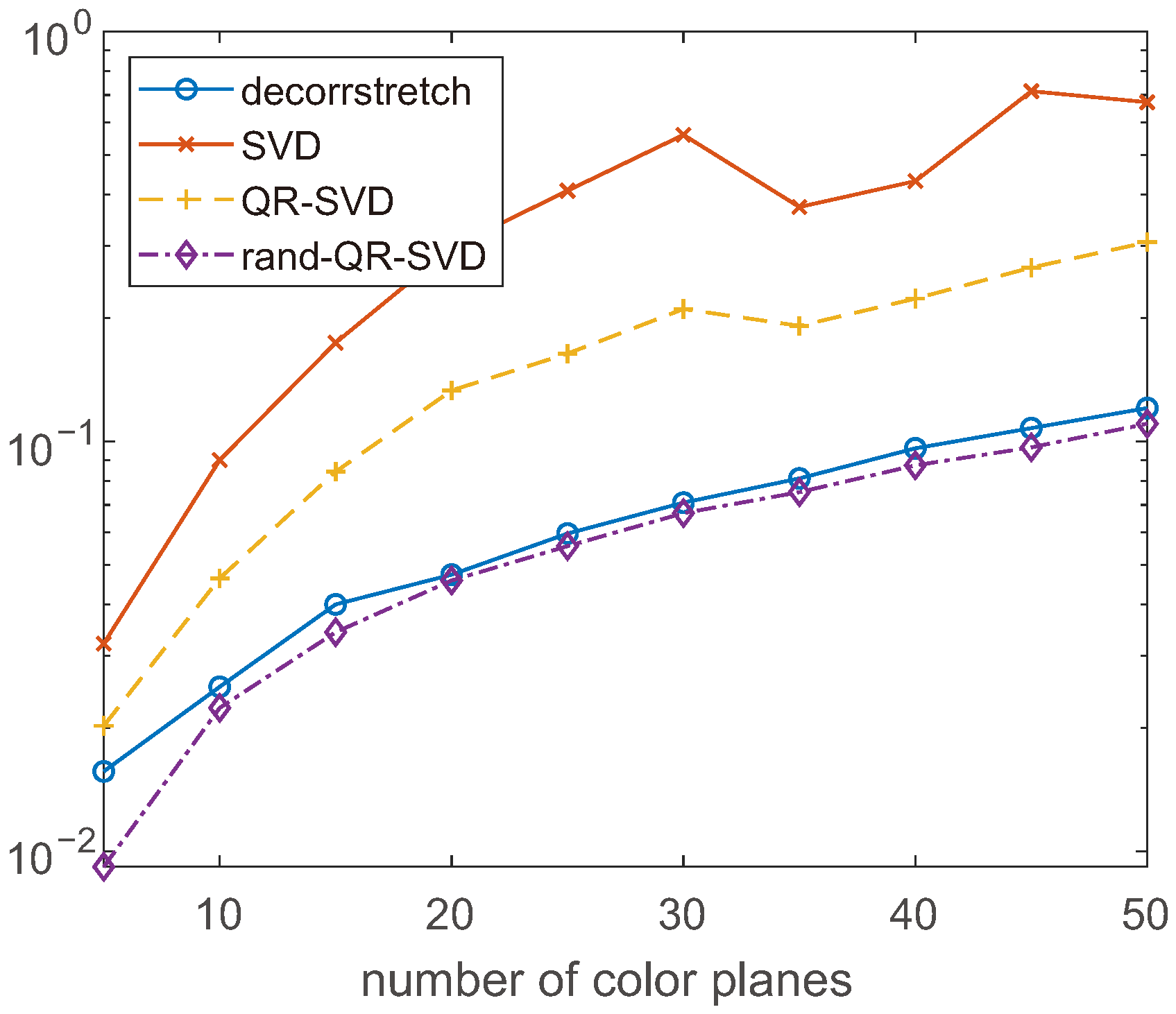
In Figure 2, we repeat the same kind of test for random multispectral images rand($1000,1000,n$), with $n=5,10,\dots ,50$, that is, for a fixed resolution and increasing number of color planes. The graph shows that the difference in the computing time between the methods increases with n, and that the randomized approach is essentially equivalent to decorrstretch. The strange behavior of the results for the SVD methods for large values of n is probably due to some kind of parallel optimization which is activated by MATLAB for large array sizes.

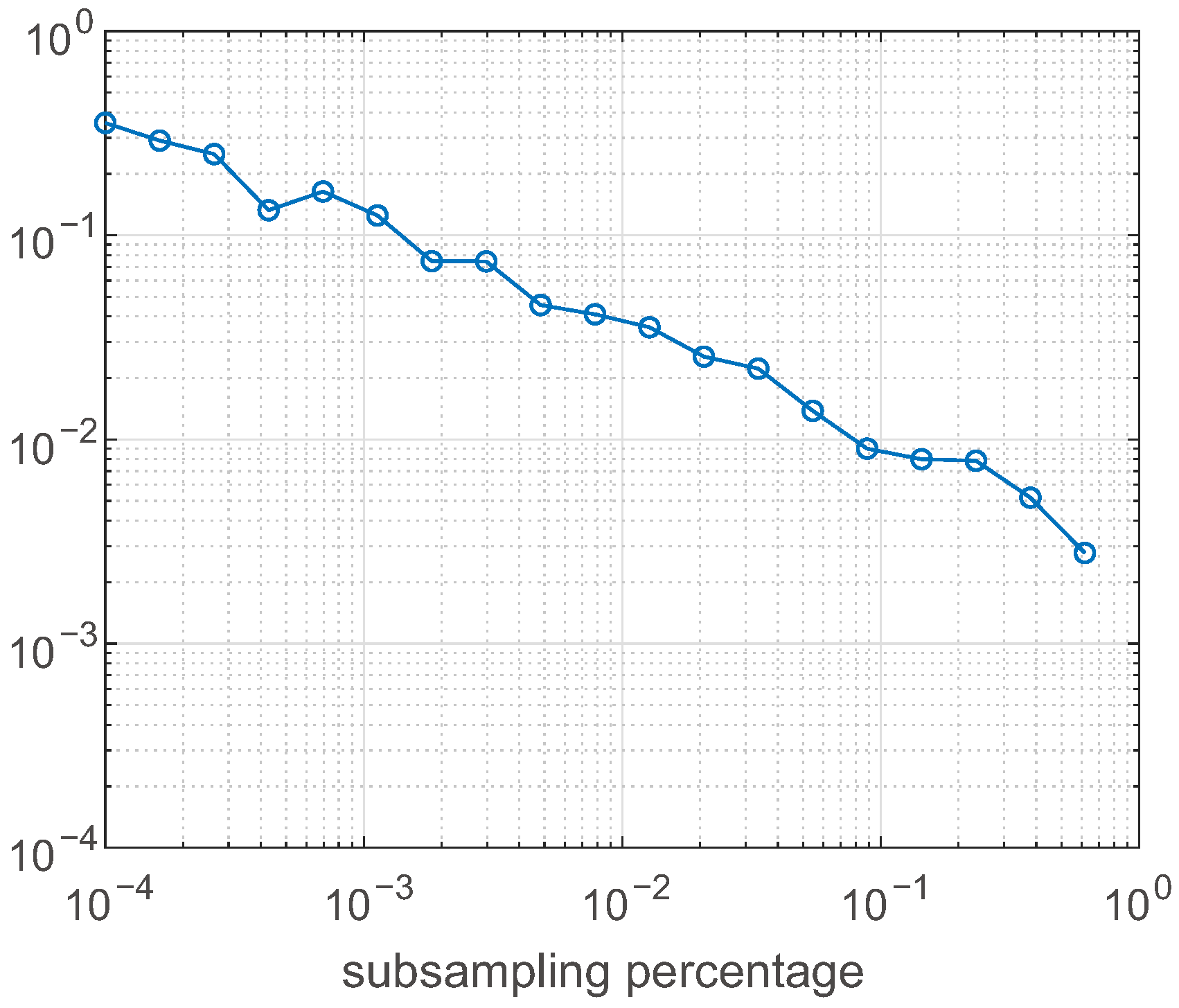
Then, we turn to analyze the error introduced by the randomized approach. In Figure 3, we show the value of the relative error

$${\displaystyle \frac{{max}_{i,j}|{\mathcal{I}}_{i,j}-{\mathcal{I}}_{i,j}^{\varphi }|}{{max}_{i,j}\left|{\mathcal{I}}_{i,j}\right|}},$$

where $\mathcal{I}$ is the output of the QR-SVD method when applied to the west test problem (resolution $394\times 369$), and ${\mathcal{I}}^{\varphi }$ is the result produced by the same method with a random subsampling of size $\lfloor \varphi p\rfloor$, for $\varphi$ logarithmically spaced between ${10}^{-4}$ and 1. 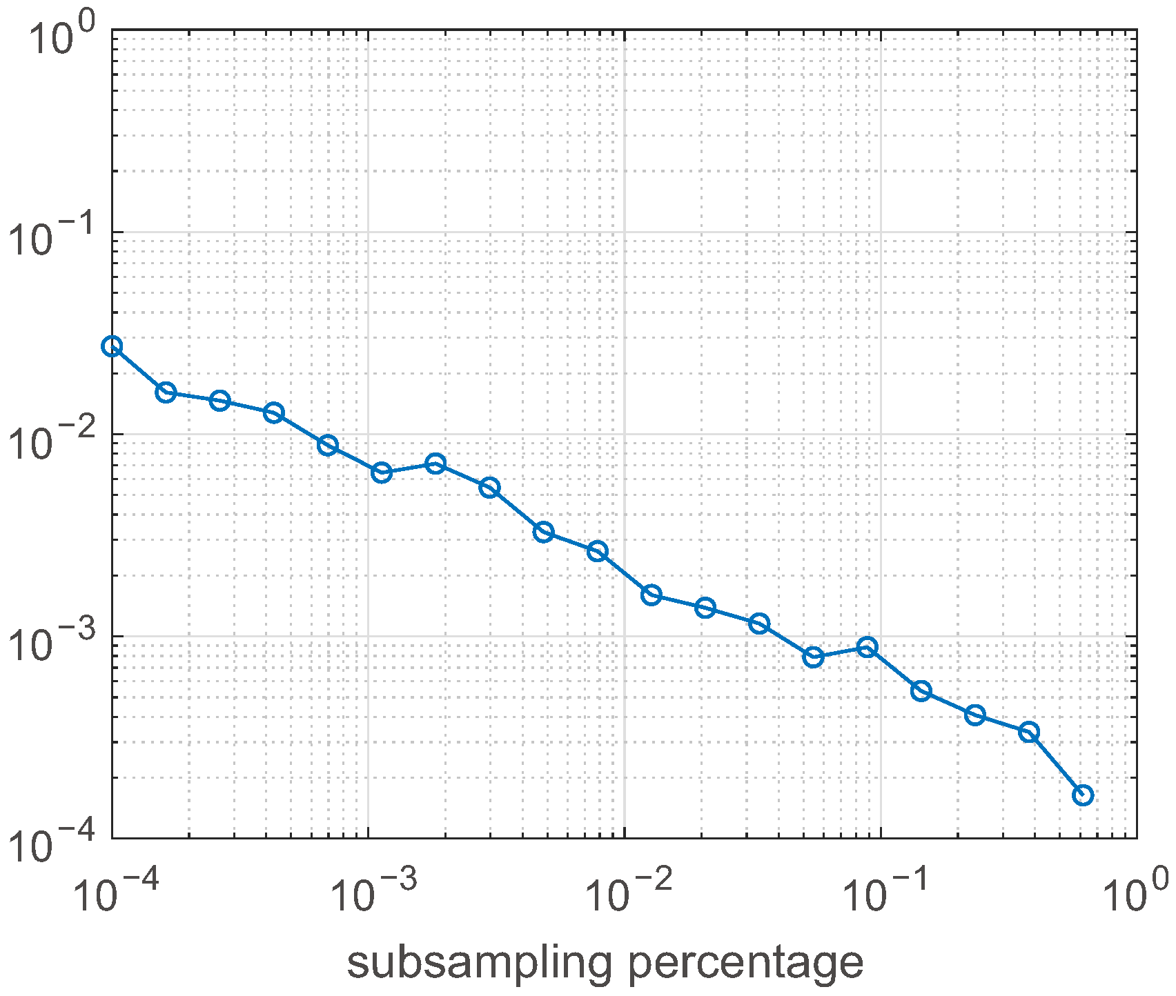For this relatively small image, $\varphi ={10}^{-3}$ roughly produces a $10\%$ error. For a large image, the error is substantially smaller, as the graph in Figure 4 shows, where the same experiment is performed on the test image pimentel, of size $4012\times 6016$.

A $10\%$ error is practically unnoticeable, as Figure 5 shows, where the original west image is displayed together with the results of decorrstretch, QR-SVD, and rand-QR-SVD, that is, the same method with a random subsampling corresponding to $\varphi ={10}^{-3}$. The three images on the right are hardly distinguishable. Indeed, the signal-to-noise ratio (SNR) between both reconstructed images and the original one is 15.54, while the randomized method produces the SNR 15.27. The fact that the two non-randomized methods are substantially equivalent is testified by a mutual SNR of 270.21.

Figure 6 shows the original pimentel image and the stretched version produced by rand-QR-SVD. Degraded paintings present on the rock wall are greatly enhanced. This helps archeologists in classifying the shapes drawn in these kinds of burial sites.

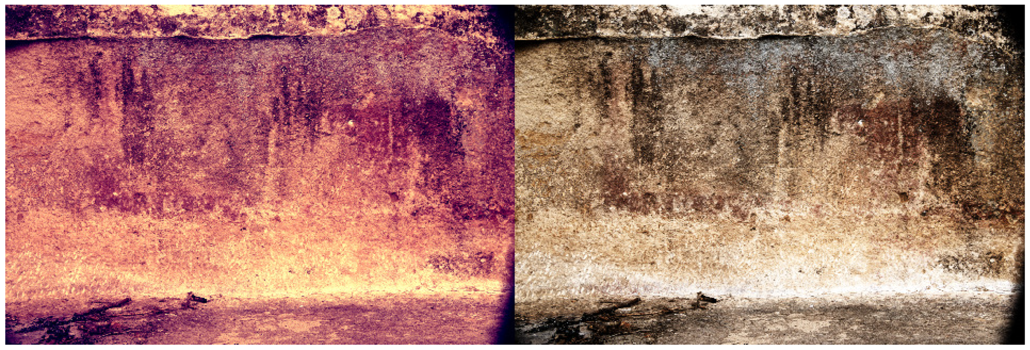
As a comparison, we display in Figure 7 the images resulting from applying to the pimentel image two other image enhancement techniques. We increased the contrast of the image by using the imadjust MATLAB function, and by histogram equalization, as implemented in the histeq function. The first approach requires user-defined intensity values for the colors, which cannot be estimated automatically. The second one does not require any parameters. It is clear that contrast enhancement methods act on images differently from DS and do not detect the presence of the painting.

The main advantage of the QR-SVD decorrelation stretch algorithm is its capability to automatically detect degenerate cases of linearly dependent color planes and correctly process them, generating pictures with uncorrelated color planes.

To investigate this aspect, we modified the west test image by making its blue color plane linearly dependent on the other two planes. We set the blue pixel values to be two times the corresponding red values plus the green ones. Figure 8 displays the modified test image together with the results of decorrstretch and QR-SVD. The last image clearly exhibits the best enhancement. The difference in the colors of the two processed images is due to the fact that once the QR-SVD method detects a linearly dependent color plane, it sets the corresponding pixels to zero in the result. The consequence is that the processed image contains only red and blue pixels. The same experiments have been performed on the pimentel image. Results are displayed in Figure 9.

To illustrate the effect of DS on a multispectral image, we processed the dataset paris. It contains a seven-band 512-by-512 Landsat image. Figure 10 shows the results obtained by the QR-SVD algorithm. We visualize bands $(1,2,3)$ (left column), $(3,4,5)$ (center column), and $(5,6,7)$ (right column). The top row reports the unprocessed color planes; the bottom row reports the results obtained by DS. To correctly display images, we adjusted them using the MATLAB function imadjust.

6. Conclusions

Decorrelation stretch is an image enhancement technique based on Principal Component Analysis. It increases color differences by removing inter-channel correlations and scaling variances to let them assume target values. It is used in many applications, e.g., remote sensing and processing of archeological images, where it is important that subtle features become more visible. In this paper, we have presented some numerical methods for its application as alternatives to the original formulation. One of the algorithms can also deal with degenerate cases, producing images with uncorrelated color channels. The computing time can be reduced by coupling a random subsampling of the image to the above method.