Research on Three-Dimensional Extension of Barzilai-Borwein-like Method

Abstract

The Barzilai-Borwein (BB) method usually uses BB stepsize for iteration so as to eliminate the line search step in the steepest descent method. In this paper, we modify the BB stepsize and extend it to solve the optimization problems of three-dimensional quadratic functions. The discussion is divided into two cases. Firstly, we study the case where the coefficient matrix of the quadratic term of quadratic function is a special third-order diagonal matrix and prove that using the new modified stepsize, this case is R-superlinearly convergent. In addition to that, we extend it to n-dimensional case and prove the rate of convergence is R-linear. Secondly, we analyze that the coefficient matrix of the quadratic term of quadratic function is a third-order asymmetric matrix, that is, when the matrix has a double characteristic root and prove the global convergence of this case. The results of numerical experiments show that the modified method is effective for the above two cases.

1. Introduction

In this paper, we consider the unconstrained optimization problem of minimizing the quadratic function,

$$\underset{x\in R^n}{\min }f\left(x\right)={\displaystyle \frac{1}{2}}{x}^{T}Ax-b^{T}x,$$

(1)

where $A\in R^{n\times n}$ is the coefficient matrix of the quadratic term, $b\in R^n$. In order to solve (1), common optimization methods usually take the following iterative approach:

$$x_{k+1}=x_k-{\alpha }_k{g}_k,$$

(2)

where $g_k=\nabla f\left(x_k\right)$, ${\alpha }_k>0$ is called stepsize. Different method has different definition of the stepsize, so the studies on stepsize are diverse. The most common method is the classical steepest descent method [1], whose stepsize is called Cauchy stepsize,

$${\alpha }_k^{SD}=\arg \underset{\alpha >0}{\min }f(x_k-\alpha g_k),$$

(3)

this method to find the stepsize is also called accurate one-dimensional line search, and Forsythe proved the rate of convergence of the classical steepest descent is linear in [2]. Although the stepsize ${\alpha }_k^{SD}$ is effective, the classical steepest descent method will not work well when the condition number of A is large, see [3] for details.

In order to ensure the convergence speed and reduce the amount of computation, Borwein and Barzilai [4] proposed a new stepsize, they turned the iterative formula into

$$x_{k+1}=x_k-D_k{g}_k,$$

(4)

where $D_k={\alpha }_{k}I$, I is identity matrix. It is similar to the quasi-Newton method [5], $D_k^{-1}$ can be regarded as an approximate Hessian matrix of f at $x_k$. And then, in order for $D_k$ to have quasi-Newton property, they chose ${\alpha }_k$ so that $D_k$ meets the following condition:

$$D_k=\arg \underset{D=\alpha I}{\min }\parallel D^{-1}{s}_{k-1}-y_{k-1}\parallel ,$$

(5)

and they have

$${\alpha }_k^{BB1}={\displaystyle \frac{s_{k-1}^T{s}_{k-1}}{s_{k-1}^T{y}_{k-1}}},$$

(6)

where $s_{k-1}=x_k-x_{k-1}$, $y_{k-1}=g_k-g_{k-1}$ and $\parallel ·\parallel$ denotes the Euclidean norm. Additionally, in another way to choose the stepsize ${\alpha }_k$, they let $D_k$ satisfy

$$D_k=\arg \underset{D=\alpha I}{\min }\parallel s_{k-1}-D{y}_{k-1}\parallel ,$$

(7)

and then they have another stepsize

$${\alpha }_k^{BB2}={\displaystyle \frac{s_{k-1}^T{y}_{k-1}}{y_{k-1}^T{y}_{k-1}}}.$$

(8)

As we can see, if $s_{k-1}^T{y}_{k-1}>0$, then ${\alpha }_k^{BB1}\ge {\alpha }_k^{BB2}$, so ${\alpha }_k^{BB1}$ is a long stepsize and ${\alpha }_k^{BB2}$ is a short stepsize. So ${\alpha }_k^{BB1}$ will perform better than ${\alpha }_k^{BB2}$ in solving some optimization problems, see [6,7] for details. And the methods that use ${\alpha }_k^{BB1}$ or ${\alpha }_k^{BB2}$ as stepsize are collectively referred to as BB methods.

In recent years, there has been a lot of research on the convergence and stepsize modification of the BB methods [8,9,10]. From previous studies, it can be found that the convergence rate of BB methods are usually R-superlinear and R-linear. For example, in [4], Barzilai and Borwein proved R-superlinear convergence of their method with the stepsize ${\alpha }_k^{BB2}$ for solving two-dimensional strictly convex quadratics. And Dai and Liao [11] proved R-linear convergence of the BB method for n-dimensional strictly convex quadratics. Now we give the definition of these two rates of convergence as follows.

Definition 1. 

Set

$$R_1=\underset{k\to \infty }{\lim \sup }{\parallel x_k-x^{*}\parallel }^{1/k}$$

(9)

According to the above formula, the R-convergence rate can be divided into two cases:

(i) When $R_1=0$, the sequence of iterated points $\left\{x_k\right\}$ is said to have R-superlinear convergence rate;

(ii) When $0<R_1<1$, the sequence of iterated points $\left\{x_k\right\}$ is said to have R-linear convergence rate.

In addition to solving quadratics, the BB method can also solve nonlinear optimization problems. Raydan [12] proposed a global Barzilai-Borwein method for unconstrained optimization problems by combining with the nonmonotone line search proposed by Grippo et al. [13]. Dai and Fletcher [14] developed projected BB methods for solving large-scale box-constrained quadratic programming. Additionally, Huang and Liu [15] extended the projected BB methods by using smoothing techniques, and they modified it to solve non-Lipschitz optimization problems. In [16], Dai considered alternating the Cauchy stepsize and the BB stepsize, and proposed an alternate step gradient method. And in [17], Zhou et al. proposed an Adaptive Barzilai-Borwein (ABB) method which alternated ${\alpha }_k^{BB1}$ and ${\alpha }_k^{BB2}$.

In addition, the relationship between BB stepsizes and the spectrum of the Hessian matrices of the objective function has also attracted wide attention. Based on the ABB method in [17], Frassoldati et al. [18] tried to use ${\alpha }_k^{BB1}$ close to the reciprocal of the minimum eigenvalue of the Hessian matrix. Their first implementation of this idea was denoted by ABBmin1 and in order to better the iteration effect, they proposed another method, denoted by ABBmin2. De Asmundis et al. [19] used the spectral property of the stepsize in [20] to propose an SDC method, the SDC indicated that the Cauchy stepsize ${\alpha }_k^{SD}$ was alternated with the Constant one. In [21], the Broyden class of quasi-Newton method approximates the inverse of the Hessian matrix by

$$H_k^{\tau }=\tau H_k^{BFGS}+(1-\tau )H_k^{DFP},$$

(10)

where $\tau \in [0,1]$, $H_k^{BFGS}$ and $H_k^{DFP}$ are the BFGS and DFP matrices satisfying the formula $H_k{y}_{k-1}=s_{k-1}$, respectively. In the quasi-Newton method, these are the two most common corrections for $H_k$. Among them, the DFP correction was first proposed by Daviden [22] and later explained and developed by Fletcher and Powell [23], while the BFGS correction was summarized from the quasi-Newton method proposed by Broyden, Fletcher, Goldfarb and Shanno independently in 1970 [24,25,26,27]. Similarly, applying this idea to the BB method, Dai et al. [28] solved the following equation

$$\underset{D=\alpha I}{\min }\parallel \tau (D^{-1}{s}_{k-1}-y_{k-1})+(1-\tau )(s_{k-1}-D{y}_{k-1})\parallel$$

(11)

to obtain the convex combination of ${\alpha }_k^{BB1}$ and ${\alpha }_k^{BB2}$

$${\alpha }_k={\gamma }_k{\alpha }_k^{BB1}+(1-{\gamma }_k){\alpha }_k^{BB2},$$

(12)

where ${\gamma }_k\in [0,1]$, and they further proved that the family of spectral gradient methods of (12) have R-superlinear convergence for two-dimensional strictly convex quadratics.

In addition to the several stepsize definitions mentioned above, there are also some BB-like stepsize. In [29], Dai et al. set $A=\left[\begin{array}{cc}1& \\ & \lambda \end{array}\right]$ and $b=\mathbf{0}$, where $\lambda >1$, they obtained a positive BB-like stepsize by averaging ${\alpha }_k^{BB1}$ and ${\alpha }_k^{BB2}$ geometrically as follows

$${\alpha }_k=\sqrt{{\alpha }_k^{BB1}·{\alpha }_k^{BB2}},$$

(13)

whose simplification is equivalent to

$${\alpha }_k={\displaystyle \frac{\parallel g_{k-1}\parallel }{\parallel A{g}_{k-1}\parallel }},$$

(14)

and they proved the R-superlinear convergence of the method. In addition, (14) can also be seen as a delay extension of the stepsize proposed by Dai and Yang in [30],

$${\alpha }_k^{DY}={\displaystyle \frac{\parallel g_k\parallel }{\parallel A{g}_k\parallel }}.$$

(15)

Interestingly, it has been shown in [30] that (15) will eventually approach the minimum value of $\parallel I-\alpha A\parallel$, precisely

$$\underset{k\to \infty }{\lim \inf }{\alpha }_k^{DY}={\displaystyle \frac{2}{{\lambda }_1+{\lambda }_n}},$$

(16)

where ${\lambda }_1$ and ${\lambda }_n$ are the minimum and maximum eigenvalues of A, and their corresponding eigenvectors are ${\displaystyle \frac{g_k}{\parallel g_k\parallel }}+{\displaystyle \frac{g_{k+1}}{\parallel g_{k+1}\parallel }}$ and ${\displaystyle \frac{g_k}{\parallel g_k\parallel }}-{\displaystyle \frac{g_{k+1}}{\parallel g_{k+1}\parallel }}$, respectively. The minimum stepsize of (16) is the optimal stepsize in [31], i.e.,

$${\alpha }_k^{OPT}=\arg \underset{\alpha \in R^1}{\min }\parallel I-\alpha A\parallel ,{\alpha }_k^{OPT}={\displaystyle \frac{2}{{\lambda }_1+{\lambda }_n}}.$$

(17)

In this paper, we mainly research on the three-dimensional cases. That is to say, the coefficient matrix A of the quadratic term is a third-order matrix. In [29], their BB-like method applied only to $A=\left[\begin{array}{cc}1& \\ & \lambda \end{array}\right]$, $\lambda >1$. Based on it, we modify the stepsize in (14) as follows:

$${\alpha }_k^{new}={\displaystyle \frac{\parallel g_{k-1}\parallel }{∥\frac{A^T+A}{2}{g}_{k-1}∥}},$$

(18)

and make it applicable to both cases $A=\left[\begin{array}{ccc}1& & \\ & 1& \\ & & \lambda \end{array}\right]$ and $A=\left[\begin{array}{ccc}1& 0& 0\\ 0& \lambda & 0\\ 0& 1& \lambda \end{array}\right]$, $\lambda >1$. For the case $A=\left[\begin{array}{ccc}1& & \\ & 1& \\ & & \lambda \end{array}\right]$, $\lambda >1$, we generalize it to a more general form which is $A=\left[\begin{array}{ccc}\mu & & \\ & \mu & \\ & & \phi \end{array}\right]$, where $\phi >\mu \ge 1$. For these two cases, we have carried out the proof of convergence and numerical experiments.

The paper is organized as follows. In Section 2, we analyze the new BB-like method which uses the stepsize ${\alpha }_k^{new}$ for the case of $A=\left[\begin{array}{ccc}1& & \\ & 1& \\ & & \lambda \end{array}\right]$, $\lambda >1$ and $A=\left[\begin{array}{ccc}\mu & & \\ & \mu & \\ & & \phi \end{array}\right]$, $\phi >\mu \ge 1$, we prove the rate of convergence of the new method is R-superlinear. Additionally, we extend this case to n-dimension, which means that $A=\mathrm{diag}\{{\lambda }_1,{\lambda }_2,\cdots ,{\lambda }_n\}$, where $1={\lambda }_1\le {\lambda }_2\le \cdots \le {\lambda }_n$. And we prove the rate of convergence in the n-dimensional case is R-linear. Section 3 provides the research of the case $A=\left[\begin{array}{ccc}1& 0& 0\\ 0& \lambda & 0\\ 0& 1& \lambda \end{array}\right]$, $\lambda >1$, and we prove the global convergence of this case under some assumption. In Section 4, we give some numerical experiment results to show the effectiveness of the new method. Finally, the conclusions are given in Section 5.

2. The Case Where A Is a Diagonal Matrix and Its Convergence Analysis

2.1. Three-Dimensional Case

In this section, we start with the basic case that

$$A=\left[\begin{array}{ccc}1& & \\ & 1& \\ & & \lambda \end{array}\right],b=\mathbf{0},$$

where $\lambda >1$. According to the iteration formula $x_{k+1}=x_k-{\alpha }_k{g}_k$, we assume that $x_1,x_2$ are given initial iteration points and they satisfy

$$g_1^{\left(i\right)}\ne 0,g_2^{\left(i\right)}\ne 0,i=1,2,3.$$

(19)

As we know,

$${\alpha }_k^{new}={\displaystyle \frac{\parallel g_{k-1}\parallel }{∥\frac{A^T+A}{2}{g}_{k-1}∥}},$$

so we have

$$\begin{array}{c}\parallel g_{k-1}\parallel =\sqrt{{\left(g_{k-1}^{\left(1\right)}\right)}^2+{\left(g_{k-1}^{\left(2\right)}\right)}^2+{\left(g_{k-1}^{\left(3\right)}\right)}^2},\\ ∥{\displaystyle \frac{A^T+A}{2}}{g}_{k-1}∥=\parallel A{g}_{k-1}\parallel =\sqrt{{\left(g_{k-1}^{\left(1\right)}\right)}^2+{\left(g_{k-1}^{\left(2\right)}\right)}^2+{\left(\lambda g_{k-1}^{\left(3\right)}\right)}^2},\\ {\alpha }_k^{new}={\displaystyle \frac{\sqrt{{\left(g_{k-1}^{\left(1\right)}\right)}^2+{\left(g_{k-1}^{\left(2\right)}\right)}^2+{\left(g_{k-1}^{\left(3\right)}\right)}^2}}{\sqrt{{\left(g_{k-1}^{\left(1\right)}\right)}^2+{\left(g_{k-1}^{\left(2\right)}\right)}^2+{\left(\lambda g_{k-1}^{\left(3\right)}\right)}^2}}}.\end{array}$$

(20)

we set

$$p_k={\displaystyle \frac{{\left(g_k^{\left(1\right)}\right)}^2+{\left(g_k^{\left(2\right)}\right)}^2}{{\left(g_k^{\left(3\right)}\right)}^2}},$$

(21)

then ${\alpha }_k^{new}$ can be written as

$${\alpha }_k^{new}={\displaystyle \frac{\sqrt{1+p_{k-1}}}{\sqrt{{\lambda }^2+p_{k-1}}}}.$$

(22)

Notice that $g_k=A{x}_k$ so the iteration formula for $g_k$ is

$$g_{k+1}=(I-{\alpha }_k^{new}A)g_k.$$

(23)

According to (23), we have

$$\begin{array}{cc}\hfill \left(\begin{array}{c}{g}_{k+1}^{\left(1\right)}\\ g_{k+1}^{\left(2\right)}\\ g_{k+1}^{\left(3\right)}\end{array}\right)& =\left(\left[\begin{array}{ccc}1& & \\ & 1& \\ & & 1\end{array}\right]-{\displaystyle \frac{\sqrt{1+p_{k-1}}}{\sqrt{{\lambda }^2+p_{k-1}}}}\left[\begin{array}{ccc}1& & \\ & 1& \\ & & \lambda \end{array}\right]\right)\left(\begin{array}{c}{g}_k^{\left(1\right)}\\ g_k^{\left(2\right)}\\ g_k^{\left(3\right)}\end{array}\right)\hfill \\ \hfill & =\left[\begin{array}{ccc}{\displaystyle \frac{\sqrt{{\lambda }^2+p_{k-1}}-\sqrt{1+p_{k-1}}}{\sqrt{{\lambda }^2+p_{k-1}}}}& & \\ & {\displaystyle \frac{\sqrt{{\lambda }^2+p_{k-1}}-\sqrt{1+p_{k-1}}}{\sqrt{{\lambda }^2+p_{k-1}}}}& \\ & & {\displaystyle \frac{\sqrt{{\lambda }^2+p_{k-1}}-\lambda \sqrt{1+p_{k-1}}}{\sqrt{{\lambda }^2+p_{k-1}}}}\end{array}\right]\left(\begin{array}{c}{g}_k^{\left(1\right)}\\ g_k^{\left(2\right)}\\ g_k^{\left(3\right)}\end{array}\right),\hfill \end{array}$$

which is equivalent to

$$\left\{\begin{array}{c}{g}_{k+1}^{\left(1\right)}=\left(1-{\displaystyle \frac{\sqrt{1+p_{k-1}}}{\sqrt{{\lambda }^2+p_{k-1}}}}\right)g_k^{\left(1\right)};\hfill \\ g_{k+1}^{\left(2\right)}=\left(1-{\displaystyle \frac{\sqrt{1+p_{k-1}}}{\sqrt{{\lambda }^2+p_{k-1}}}}\right)g_k^{\left(2\right)};\hfill \\ g_{k+1}^{\left(3\right)}=\left(1-{\displaystyle \frac{\lambda \sqrt{1+p_{k-1}}}{\sqrt{{\lambda }^2+p_{k-1}}}}\right)g_k^{\left(3\right)}.\hfill \end{array}\right.$$

(24)

From (21) and (24), we can obtain

$$\begin{array}{cc}\hfill p_{k+1}& ={\displaystyle \frac{{\left(g_{k+1}^{\left(1\right)}\right)}^2+{\left(g_{k+1}^{\left(2\right)}\right)}^2}{{\left(g_{k+1}^{\left(3\right)}\right)}^2}}\hfill \\ & ={\displaystyle \frac{{\left(1-\frac{\sqrt{1+p_{k-1}}}{\sqrt{{\lambda }^2+p_{k-1}}}\right)}^2\left[{\left(g_k^{\left(1\right)}\right)}^2+{\left(g_k^{\left(2\right)}\right)}^2\right]}{{\left(1-\frac{\lambda \sqrt{1+p_{k-1}}}{\sqrt{{\lambda }^2+p_{k-1}}}\right)}^2{\left(g_k^{\left(3\right)}\right)}^2}}\hfill \\ & ={\displaystyle \frac{{\left(1-\frac{\sqrt{1+p_{k-1}}}{\sqrt{{\lambda }^2+p_{k-1}}}\right)}^2}{{\left(1-\frac{\lambda \sqrt{1+p_{k-1}}}{\sqrt{{\lambda }^2+p_{k-1}}}\right)}^2}}{p}_k\hfill \\ & ={\left({\displaystyle \frac{\sqrt{{\lambda }^2+p_{k-1}}-\sqrt{1+p_{k-1}}}{\sqrt{{\lambda }^2+p_{k-1}}-\lambda \sqrt{1+p_{k-1}}}}\right)}^2{p}_k\hfill \\ & ={\left({\displaystyle \frac{(\sqrt{{\lambda }^2+p_{k-1}}-\sqrt{1+p_{k-1}})(\sqrt{{\lambda }^2+p_{k-1}}+\lambda \sqrt{1+p_{k-1}})}{({\lambda }^2-1)p_{k-1}}}\right)}^2{p}_k\hfill \\ & ={\left({\displaystyle \frac{\lambda -p_{k-1}+\sqrt{\tau \left(p_{k-1}\right)}}{\lambda +1}}\right)}^2{\displaystyle \frac{p_k}{p_{k-1}^2}},\hfill \end{array}$$

(25)

where $\tau$ is a quadratic function

$$\tau \left(\nu \right)=(1+\nu )({\lambda }^2+\nu ),\nu >0.$$

(26)

Let

$$h\left(\nu \right)={\displaystyle \frac{\lambda -\nu +\sqrt{\tau \left(\nu \right)}}{\lambda +1}},\nu >0,$$

(27)

then

$$p_{k+1}={\left(h\left(p_{k-1}\right)\right)}^2{\displaystyle \frac{p_k}{p_{k-1}^2}}.$$

(28)

We define $W_k=\log p_k$, by (28) we have

$$W_{k+1}=W_k-2W_{k-1}+2\log h\left(p_{k-1}\right).$$

(29)

In order to prove the R-superlinear convergence of this case, we give three Lemma firstly.

Lemma 1. 

Assume that $\lambda >1$, the function $h\left(\nu \right)$ is monotonically increasing and $h\left(\nu \right)\in \left({\displaystyle \frac{2\lambda }{\lambda +1}},{\displaystyle \frac{\lambda +1}{2}}\right)$ when $\nu \in (0,+\infty )$.

Proof. 

The proof of Lemma 1 can fully refer to the proof of Lemma 1.2.1 in [29].

According to (26), we have

$${\tau }^{\prime }=(1+\nu )+({\lambda }^2+\nu ),$$

and

$${\left({\tau }^{\prime }\right)}^2-4\tau ={({\lambda }^2-1)}^2.$$

(30)

By direct calculation, we can obtain

$$\begin{array}{cc}\hfill h^{\prime }\left(\nu \right)& ={\displaystyle \frac{-1+\frac{1}{2}{\tau }^{-\frac{1}{2}}{\tau }^{\prime }}{\lambda +1}}\hfill \\ & ={\displaystyle \frac{{\left({\tau }^{\prime }\right)}^2-4\tau }{2(\lambda +1){\tau }^{\frac{1}{2}}({\tau }^{\prime }+2{\tau }^{\frac{1}{2}})}}\hfill \\ \hfill & ={\displaystyle \frac{{({\lambda }^2-1)}^2}{2(\lambda +1)({\tau }^{\frac{1}{2}}{\tau }^{\prime }+2\tau )}}.\hfill \end{array}$$

(31)

Since $\nu \ge 0$, we have $h^{\prime }\left(\nu \right)>0$. So $h\left(\nu \right)$ is monotonically increasing and when $\nu =0$, we have

$$h\left(0\right)={\displaystyle \frac{2\lambda }{\lambda +1}}.$$

In addition to that, we have

$$\underset{\nu \to \infty }{\lim }h\left(\nu \right)={\displaystyle \frac{\lambda +1}{2}}.$$

So in summary, we obtain that when $\nu \ge 0$, $h\left(\nu \right)\in \left({\displaystyle \frac{2\lambda }{\lambda +1}},{\displaystyle \frac{\lambda +1}{2}}\right)$. □

In the next Lemma we will give the definition of ${\zeta }_k$ and its lower bound.

Lemma 2. 

We define ${\zeta }_k=W_k+(\gamma -1)W_{k-1}$, where γ satisfies ${\gamma }^2-\gamma +2=0$, if

$$|{\zeta }_2| >8\log {\displaystyle \frac{\lambda +1}{2}},$$

(32)

then there exists $c_1>0$, such that

$$|{\zeta }_k| >(\sqrt{2}-1)2^{{\displaystyle \frac{k}{2}}}{c}_1,k\ge 2.$$

(33)

Proof. 

According to the definition of ${\zeta }_k$ and (29),

$$\begin{array}{cc}\hfill {\zeta }_{k+1}& =\gamma W_k+W_{k+1}-W_k\hfill \\ & =\gamma W_k-2W_{k-1}+2\log h\left(p_{k-1}\right)\hfill \\ & =\gamma {\zeta }_k+2\log h\left(p_{k-1}\right).\hfill \end{array}$$

Notice that $\left|\gamma \right|=\sqrt{2}$, and from Lemma 1 we have $\log h\left(p_{k-1}\right)<\log {\displaystyle \frac{\lambda +1}{2}}$, so

$$|{\zeta }_{k+1}|>\sqrt{2}\left|{\zeta }_k\right|-c_1,$$

where $c_1=2\log {\displaystyle \frac{\lambda +1}{2}}$. By (32), we can obtain

$$\begin{array}{cc}\hfill |{\zeta }_{k+1}|& \ge 2^{{\displaystyle \frac{k-1}{2}}}\left|{\zeta }_2\right|-{\displaystyle \frac{2^{\frac{k}{2}}-1}{\sqrt{2}-1}}{c}_1\hfill \\ & \ge \left(2^{{\displaystyle \frac{k+3}{2}}}-{\displaystyle \frac{2^{\frac{k}{2}}-1}{\sqrt{2}-1}}\right)c_1\hfill \\ & =[(\sqrt{2}-1)(2^{{\displaystyle \frac{k}{2}}}+1)+2]c_1\hfill \\ & >(\sqrt{2}-1)2^{{\displaystyle \frac{k}{2}}}{c}_1,\hfill \end{array}$$

so we finish the proof. □

By the Lemma 2 we know $\gamma ={\displaystyle \frac{1\pm \sqrt{7}i}{2}}$ and $|\gamma -1|=\sqrt{2}$, so

$$|{\zeta }_k\left|\le \right|W_k\left|+\sqrt{2}|W_{k-1}\right|\le (\sqrt{2}+1)\max \{\left|W_k\right|,\left|W_{k-1}\right|\},$$

combining it with (33) we can obtain

$$\max \left\{\right|W_k|,|W_{k-1}\left|\right\}\ge {\displaystyle \frac{1}{\sqrt{2}+1}}(\sqrt{2}-1)2^{{\displaystyle \frac{k}{2}}}{c}_1={(\sqrt{2}-1)}^2{2}^{{\displaystyle \frac{k}{2}}}{c}_1.$$

(34)

Lemma 3. 

Under the conditions of Lemma 2, we have

$$\underset{-1\le i\le 3}{\max }{W}_{k+i}\ge {(\sqrt{2}-1)}^2{2}^{{\displaystyle \frac{k}{2}}}{c}_1-4\log {\displaystyle \frac{\lambda +1}{2}},k\ge 2;$$

(35)

$$\underset{-1\le i\le 3}{\min }{W}_{k+i}\le -{(\sqrt{2}-1)}^2{2}^{{\displaystyle \frac{k}{2}}}{c}_1+4\log {\displaystyle \frac{\lambda +1}{2}},k\ge 2.$$

(36)

Proof. 

By (34), if

$$W_{k-1}\ge {(\sqrt{2}-1)}^2{2}^{{\displaystyle \frac{k}{2}}}{c}_1$$

or

$$W_k\ge {(\sqrt{2}-1)}^2{2}^{{\displaystyle \frac{k}{2}}}{c}_1$$

holds, thus (35) holds. Now, we consider other cases. We assume that the above two inequalities are not true, so we have

$$W_{k-1}\le -{(\sqrt{2}-1)}^2{2}^{{\displaystyle \frac{k}{2}}}{c}_1$$

or

$$W_k\le -{(\sqrt{2}-1)}^2{2}^{{\displaystyle \frac{k}{2}}}{c}_1,$$

and by (29) we know that

$$\begin{array}{cc}\hfill W_{k+2}& =W_{k+1}-2W_k+2\log h\left(p_k\right)\hfill \\ & =-W_k-2W_{k-1}+2\log h\left(p_{k-1}\right)+2\log h\left(p_k\right).\hfill \end{array}$$

(37)

Next, we prove (35) in two cases.

Case (i). When $W_{k-1}\le -{(\sqrt{2}-1)}^2{2}^{{\displaystyle \frac{k}{2}}}{c}_1$, if $W_k<0$, we can obtain from (37)

$$W_{k+2}\ge -2W_{k-1}+2\log h\left(p_{k-1}\right)\ge {(\sqrt{2}-1)}^2{2}^{{\displaystyle \frac{k}{2}}}{c}_1-2c_1;$$

and if $W_k>0$, by (29) we have

$$W_{k+1}\ge -2W_{k-1}+2\log h\left(p_{k-1}\right)\ge {(\sqrt{2}-1)}^2{2}^{{\displaystyle \frac{k}{2}}}{c}_1-2c_1.$$

Case (ii). When $W_k\le -{(\sqrt{2}-1)}^2{2}^{{\displaystyle \frac{k}{2}}}{c}_1$, if $W_{k+1}<0$, we can obtain from (37)

$$W_{k+3}\ge -2W_k+2\log h\left(p_k\right)\ge {(\sqrt{2}-1)}^2{2}^{{\displaystyle \frac{k}{2}}}{c}_1-2c_1;$$

and if $W_{k+1}>0$, by (29) we have

$$W_{k+2}\ge -2W_k+2\log h\left(p_k\right)\ge {(\sqrt{2}-1)}^2{2}^{{\displaystyle \frac{k}{2}}}{c}_1-2c_1.$$

From the proof of Lemma 2, we know that $c_1=2\log {\displaystyle \frac{\lambda +1}{2}}$. Therefore, according to the above analysis, we can prove that (35) is true and the proof of (36) is similar to it. □

In the following theorem, we will prove the rate of convergence of this case is R-superlinear.

Theorem 1. 

Assume that (19) and (21) hold, the sequence of gradient norms $\{\parallel g_k\parallel \}$ converges to zero and it converges R-superlinearly.

Proof. 

Notice that ${\alpha }_k^{new}\in ({\displaystyle \frac{1}{\lambda }},1)$ and $g_{k+1}=(I-{\alpha }_k^{new}A)g_k$, so we can obtain

$$|g_{k+1}^{\left(i\right)}|\le (\lambda -1)|g_k^{\left(i\right)}|,$$

(38)

where $i=1,2,3$ and $k\ge 0$.

Firstly, we consider the third component of the gradient. From (24) we know

$$\begin{array}{cc}\hfill |g_{k+1}^{\left(3\right)}|& \le \left|{\displaystyle \frac{\sqrt{{\lambda }^2+p_{k-1}}-\lambda \sqrt{1+p_{k-1}}}{\sqrt{{\lambda }^2+p_{k-1}}}}\right|\left|g_k^{\left(3\right)}\right|\hfill \\ & \le {\displaystyle \frac{({\lambda }^2-1)p_{k-1}}{\sqrt{{\lambda }^2+p_{k-1}}(\sqrt{{\lambda }^2+p_{k-1}}+\lambda \sqrt{1+p_{k-1}})}}\left|g_k^{\left(3\right)}\right|\hfill \\ & \le {\displaystyle \frac{({\lambda }^2-1)p_{k-1}}{2{\lambda }^2}}\left|g_k^{\left(3\right)}\right|\hfill \\ & <(\lambda -1)p_{k-1}\left|g_k^{\left(3\right)}\right|.\hfill \end{array}$$

(39)

Combining (38) and (39), we obtain

$$|g_{k+5}^{\left(3\right)}{| \le (\lambda -1)}^5(\underset{-1\le j\le 3}{\min }{p}_{k+j})\left|g_k^{\left(3\right)}\right|.$$

(40)

Since $W_k=\log p_k$, so by using (36) we have

$$|g_{(k+5)}^{\left(3\right)}{| \le (\lambda -1)}^5\exp \left(-{(\sqrt{2}-1)}^2{2}^{{\displaystyle \frac{k}{2}}}{c}_1+4\log {\displaystyle \frac{\lambda +1}{2}}\right)\left|g_k^{\left(3\right)}\right|.$$

(41)

Similarly, as for the first component of the gradient, we calculate directly,

$$\begin{array}{cc}\hfill |g_{k+1}^{\left(1\right)}|& \le \left|{\displaystyle \frac{\sqrt{{\lambda }^2+p_{k-1}}-\sqrt{1+p_{k-1}}}{\sqrt{{\lambda }^2+p_{k-1}}}}\right|\left|g_k^{\left(1\right)}\right|\hfill \\ & \le {\displaystyle \frac{{\lambda }^2-1}{\sqrt{{\lambda }^2+p_{k-1}}(\sqrt{{\lambda }^2+p_{k-1}}+\sqrt{1+p_{k-1}})}}\left|g_k^{\left(1\right)}\right|\hfill \\ & \le {\displaystyle \frac{{\lambda }^2-1}{\sqrt{p_{k-1}}\left[\sqrt{p_{k-1}}\left(\sqrt{\frac{{\lambda }^2}{p_{k-1}}+1}+\sqrt{\frac{1}{p_{k-1}}+1}\right)\right]}}\left|g_k^{\left(1\right)}\right|\hfill \\ & \le {\displaystyle \frac{{\lambda }^2-1}{2p_{k-1}}}\left|g_k^{\left(1\right)}\right|.\hfill \end{array}$$

By (38) and $W_k=\log p_k$, we can obtain

$$\begin{array}{cc}\hfill |g_{k+5}^{\left(1\right)}|& \le {\displaystyle \frac{1}{2}}(\lambda +1){(\lambda -1)}^5\left(\underset{-1\le j\le 3}{\max }{\displaystyle \frac{1}{p_{k+j}}}\right)\left|g_k^{\left(1\right)}\right|\hfill \\ & \le {\displaystyle \frac{1}{2}}(\lambda +1){(\lambda -1)}^5\exp \left(-{(\sqrt{2}-1)}^2{2}^{{\displaystyle \frac{k}{2}}}{c}_1+4\log {\displaystyle \frac{\lambda +1}{2}}\right)\left|g_k^{\left(1\right)}\right|.\hfill \end{array}$$

(42)

And from (24) we know that the condition of the second component of the gradient is the same as the first component, so

$$|g_{k+5}^{\left(2\right)}| \le {\displaystyle \frac{1}{2}}(\lambda +1){(\lambda -1)}^5\exp \left(-{(\sqrt{2}-1)}^2{2}^{{\displaystyle \frac{k}{2}}}{c}_1+4\log {\displaystyle \frac{\lambda +1}{2}}\right)\left|g_k^{\left(2\right)}\right|$$

(43)

can be obtained.

Finally, by (41)–(43), for any k,

$$\parallel g_{k+5}\parallel \le {\displaystyle \frac{1}{2}}(\lambda +1){(\lambda -1)}^5\exp \left(-{(\sqrt{2}-1)}^2{2}^{{\displaystyle \frac{k}{2}}}{c}_1+4\log {\displaystyle \frac{\lambda +1}{2}}\right)\parallel g_k\parallel ,$$

(44)

so the sequence $\{\parallel g_k\parallel \}$ converges to zero R-superlinearly. □

On the basis of the above conclusion we generalize this case to a more general form, we set $A=\left[\begin{array}{ccc}\mu & & \\ & \mu & \\ & & \phi \end{array}\right]$, $\phi >\mu \ge 1$. According to the assumptions and conditions mentioned above, we have

$${\alpha }_k^{new}={\displaystyle \frac{\sqrt{{\left(g_{k-1}^{\left(1\right)}\right)}^2+{\left(g_{k-1}^{\left(2\right)}\right)}^2+{\left(g_{k-1}^{\left(3\right)}\right)}^2}}{\sqrt{{\left(\mu g_{k-1}^{\left(1\right)}\right)}^2+{\left(\mu g_{k-1}^{\left(2\right)}\right)}^2+{\left(\phi g_{k-1}^{\left(3\right)}\right)}^2}}}.$$

Substituting $p_k$ of (21) into the above equation, then

$${\alpha }_k^{new}={\displaystyle \frac{\sqrt{1+p_{k-1}}}{\sqrt{{\phi }^2+{\mu }^2{p}_{k-1}}}}.$$

According to (23), we have

$$\left\{\begin{array}{c}{g}_{k+1}^{\left(1\right)}=\left(1-{\displaystyle \frac{\mu \sqrt{1+p_{k-1}}}{\sqrt{{\phi }^2+{\mu }^2{p}_{k-1}}}}\right)g_k^{\left(1\right)};\hfill \\ g_{k+1}^{\left(2\right)}=\left(1-{\displaystyle \frac{\mu \sqrt{1+p_{k-1}}}{\sqrt{{\phi }^2+{\mu }^2{p}_{k-1}}}}\right)g_k^{\left(2\right)};\hfill \\ g_{k+1}^{\left(3\right)}=\left(1-{\displaystyle \frac{\phi \sqrt{1+p_{k-1}}}{\sqrt{{\phi }^2+{\mu }^2{p}_{k-1}}}}\right)g_k^{\left(3\right)}.\hfill \end{array}\right.$$

Using the calculation method of (25), we can obtain

$$p_{k+1}={\left({\displaystyle \frac{\phi -\mu p_{k-1}+\sqrt{\eta \left(p_{k-1}\right)}}{\phi +\mu }}\right)}^2{\displaystyle \frac{p_k}{p_{k-1}^2}},$$

where $\eta$ is a quadratic function

$$\eta \left(\omega \right)=(1+\omega )({\phi }^2+{\mu }^2\omega ),\omega >0.$$

Let

$$\theta \left(\omega \right)={\displaystyle \frac{\phi -\mu \omega +\sqrt{\eta \left(\omega \right)}}{\phi +\mu }},\omega >0,$$

then

$$p_{k+1}={\left(\theta \left(p_{k-1}\right)\right)}^2{\displaystyle \frac{p_k}{p_{k-1}^2}}.$$

So we obtain something similar to (28), and by using the same proof method as Lemmas 1–3 and Theorem 1, we can also prove that when $A=\left[\begin{array}{ccc}\mu & & \\ & \mu & \\ & & \phi \end{array}\right]$, $\phi >\mu \ge 1$, the BB-like method using the new stepsize is convergent and the rate of convergence is R-superlinear.

2.2. n-Dimensional Case

In this case, we consider that

$$A=\mathrm{diag}\{{\lambda }_1,{\lambda }_2,\cdots ,{\lambda }_n\},b=\mathbf{0},$$

where $1={\lambda }_1\le {\lambda }_2\le \cdots \le {\lambda }_n$. Then, we will prove R-linear convergence of the new method for n-dimensional case.

In [16], Dai has proved that if $A=\mathrm{diag}\{{\lambda }_1,{\lambda }_2,\cdots ,{\lambda }_n\}$, where $1={\lambda }_1\le {\lambda }_2\le \cdots \le {\lambda }_n$, and the stepsize ${\alpha }_k$ has the following Property 1, then either $g_k=0$ for some finite k or the sequence of gradient norms $\{\parallel g_k\parallel \}$ converges to zero R-linearly.

Firstly, we give the Property 1 and the Theorem in [16]. In the Property 1, they define $g_k^{\left(i\right)}$ is the ith component of $g_k$ and

$$G(k,l)=\sum _{i=1}^l{\left(g_k^{\left(i\right)}\right)}^2.$$

Property 1 

([16]). Suppose that there exist an integer m and positive constants $M_1>{\lambda }_1$ and $M_2$ such that

(i) ${\lambda }_1\le {\alpha }_k^{-1}\le M_1$;

(ii) for any integer $l\in [1,n-1]$ and $ϵ>0$, if $G(k-j,l)\le ϵ$ and ${\left(g_{k-j}^{(l+1)}\right)}^2\ge M_2ϵ$ hold for $j\in [0,\min \{k,m\}-1]$, then ${\alpha }_k^{-1}\ge {\displaystyle \frac{2}{3}}{\lambda }_{l+1}$.

Theorem 2 

([16]). Consider the linear system

$$Ax=b,A\in R^{n\times n},b\in R^n,$$

where $A=diag({\lambda }_1,{\lambda }_2,\cdots ,{\lambda }_n)$, and $1={\lambda }_1\le {\lambda }_2\cdots \le {\lambda }_n$. Consider the gradient method where the stepsize ${\alpha }_k$ has Property 1. Then either $g_k=0$ for some finite k, or the sequence $\{\parallel g_k\parallel \}$ converges to zero R-linearly.

Proof. 

The proof can fully refer to the proof of Theorem 4.1 in [16].

By (23), we have

$$g_{k+1}^{\left(i\right)}=(1-{\alpha }_k{\lambda }_i)g_k^{\left(i\right)}.$$

(45)

Denote ${\delta }_1=\max \{{(1-({\lambda }_1/M_1))}^2,1/4\}\in (0,1)$ and ${\delta }_2=\max \{{(1-(M_1/{\lambda }_1))}^2,2\}$. Then by (45) and the definition of $G(k,l)$, we can obtain that for all $k\ge 1$,

$$G(k+1,1)\le {\delta }_{1}G(k,l),$$

(46)

$${\left(g_{k+1}^{\left(i\right)}\right)}^2\le {\delta }_2{\left(g_k^{\left(i\right)}\right)}^2,\mathrm{for}i=1,2,\cdots ,n,$$

(47)

$$\parallel g_{k+1}{\parallel }^2\le {\delta }_2{\parallel g_k\parallel }^2.$$

(48)

The rest of the proof will be divided into three parts as follows:

(I). We prove that, for any integer $1\le l<n$ and $k\ge 1$, if there exist some ${ϵ}_l\in (0,M_2^{-1})$ and integer $m_l$ such that

$$G(k+j,l)\le {ϵ}_l{\parallel g_k\parallel }^2,\mathrm{for}\mathrm{all}j\ge m_l,$$

(49)

then we must have

$${\left(g_{k+j_0}^{(l+1)}\right)}^2\le M_2{ϵ}_l{\parallel g_k\parallel }^2,\mathrm{for}\mathrm{some}{j}_0\in [m_l,m_l+m+{\Delta }_l+1],$$

(50)

where

$${\Delta }_l=⌈{\displaystyle \frac{\log \left(M_2{ϵ}_l{\delta }_2^{-(m_l+m)}\right)}{\log {\delta }_1}}⌉.$$

In fact, suppose that

$${\left(g_{k+j}^{(l+1)}\right)}^2>M_2{ϵ}_l{\parallel g_k\parallel }^2,\mathrm{for}j\in [m_l,m_l+m+{\Delta }_l].$$

(51)

Then we have from (49), (51) and Property 1 (ii) that

$${\alpha }_{k+j}^{(-1)}\ge {\displaystyle \frac{2}{3}}{\lambda }_{l+1},\mathrm{for}j\in [m_l+m,m_l+m+{\Delta }_l].$$

(52)

By (45), (52) and Property 1 (i), we can obtain

$${\left(g_{k+j+1}^{(l+1)}\right)}^2\le {\delta }_1{\left(g_{k+j}^{(l+1)}\right)}^2,\mathrm{for}j\in [m_l+m,m_l+m+{\Delta }_l].$$

(53)

And from (47), (53) and the definition of ${\Delta }_l$, we obtain that

$${\left(g_{k+m_l+m+{\Delta }_l+1}^{(l+1)}\right)}^2\le {\delta }_1^{{\Delta }_l+1}{\left(g_{k+m_l+m}^{(l+1)}\right)}^2\le {\delta }_1^{{\Delta }_l+1}{\delta }_2^{m_l+m}{\left(g_k^{(l+1)}\right)}^2\le M_2{ϵ}_l{\parallel g_k\parallel }^2.$$

So (50) must hold.

(II). Denoting $m_{l+1}=m_l+m+{\Delta }_l+1$ and ${ϵ}_{l+1}=(1+M_2{\delta }_2^m){ϵ}_l$, we prove that if (49) holds, we can further have

$$G(k+j,l+1)\le {ϵ}_{l+1}{\parallel g_k\parallel }^2,\mathrm{for}\mathrm{all}j\ge m_{l+1}.$$

(54)

In fact, by (I), we know that there are infinitely many integers $j_1$ and $j_2$ with $j_2>j_1\ge j_0$ such that

$${\left(g_{k+j}^{(l+1)}\right)}^2\le M_2{ϵ}_l{\parallel g_k\parallel }^2,\mathrm{for}j=j_1,j_2,$$

(55)

and

$${\left(g_{k+j}^{(l+1)}\right)}^2>M_2{ϵ}_l{\parallel g_k\parallel }^2,\mathrm{for}j\in [j_1+1,j_2-1].$$

(56)

Then we have from (47) and (55) that

$${\left(g_{k+j}^{(l+1)}\right)}^2\le {\delta }_2^m{\left(g_{k+j_1}^{(l+1)}\right)}^2\le M_2{\delta }_2^m{ϵ}_l{\parallel g_k\parallel }^2,\mathrm{for}j\in [j_1+1,j_1+m].$$

(57)

If $j_2>j_1+m$, by Property (A), (45), (49) and (56), we have

$${\alpha }_{k+j}^{-1}\ge {\displaystyle \frac{2}{3}}{\lambda }_{l+1}\mathrm{and}{\left(g_{k+j+1}^{(l+1)}\right)}^2\le {\delta }_1{\left(g_{k+j}^{(l+1)}\right)}^2,\mathrm{for}j\in [j_1+m,j_2-1].$$

(58)

It follows from (48), (55) and (58) that

$${\left(g_{k+j}^{(l+1)}\right)}^2<{\left(g_{k+j_1+m}^{(l+1)}\right)}^2\le M_2{\delta }_2^m{ϵ}_l{\parallel g_k\parallel }^2,\mathrm{for}j\in [j_1+m+1,j_2].$$

(59)

Due to the arbitrariness of $j_1$ and $j_2$, (57) and (59), we know that the following inequality holds for any $j\ge j_0$:

$${\left(g_{k+j}^{(l+1)}\right)}^2\le M_2{\delta }_2^m{ϵ}_l{\parallel g_k\parallel }^2.$$

(60)

Since $j_0\le m_{l+1}$, then can obtain from (49), (60) and the definition of $G(k,l)$ that (54) holds.

(III). Denoting for any $1\le l\le n$,

$${ϵ}_l={\displaystyle \frac{1}{4}}{(1+M_2{\delta }_2^m)}^{(l-n)},$$

(61)

and setting $m_1=\lceil \log {ϵ}_1/\log {\delta }_1\rceil$, $m_{l+1}=m_l+m+{\Delta }_l+1$ for $l=1,\cdots ,n-1$ and $M=m_n$, we prove by induction that for all $1\le l\le n$,

$$G(k+j,l)\le {ϵ}_l{\parallel g_k\parallel }^2,\mathrm{for}\mathrm{all}j\ge m_l.$$

(62)

In fact, by (46) and the definition of $m_1$, (62) holds clearly holds for $l=1$. Suppose that (62) is true for some $1\le l\le n-1$. Then by (II), we know that (62) holds for $l+1$. Thus by induction, we know that (62) holds for all $1\le l\le n$. Notice that ${ϵ}_n=1/4$ and $G(k,n)=\parallel g_k{\parallel }^2$. It follows from (62) that

$$\parallel g_{k+M}{\parallel }^2 \le {\displaystyle \frac{1}{4}}{\parallel g_k\parallel }^2.$$

(63)

Since $M=m_n$ depends only on ${\lambda }_1$, $M_1$ and $M_2$, then we can obtain by (48) and (63) that the sequence $\{\parallel g_k\parallel \}$ converges to zero R-linearly. □

According to the Property and the Theorem given above, we will prove that the stepsize ${\alpha }_k^{new}$ satisfies Property 1 and the n-dimensional case has R-linear convergence rate in the following Theorem.

Theorem 3. 

If $A=\mathrm{diag}\{{\lambda }_1,{\lambda }_2,\cdots ,{\lambda }_n\}$, where $1={\lambda }_1\le {\lambda }_2\le \cdots \le {\lambda }_n$, then either $g_k=0$ for some finite k or the sequence of gradient norms $\{\parallel g_k\parallel \}$ converges to zero R-linearly.

Proof. 

Firstly, we let $M_1={\lambda }_n$ and $M_2=2$. When A is a symmetric positive matrix, we can obtain from (6) and (8) that

$$\begin{array}{c}{\alpha }_k^{BB1}={\displaystyle \frac{g_{k-1}^T{g}_{k-1}}{g_{k-1}^{T}A{g}_{k-1}}},\\ {\alpha }_k^{BB2}={\displaystyle \frac{g_{k-1}^{T}A{g}_{k-1}}{g_{k-1}^T{A}^2{g}_{k-1}}}.\end{array}$$

And from (18), we have

$${\alpha }_k^{new}={\displaystyle \frac{\parallel g_{k-1}\parallel }{∥\frac{A^T+A}{2}{g}_{k-1}∥}}={\displaystyle \frac{\parallel g_{k-1}\parallel }{\parallel A{g}_{k-1}\parallel }}=\sqrt{{\alpha }_k^{BB1}·{\alpha }_k^{BB2}}.$$

So, the following formula holds

$${\alpha }_k^{BB2}\le {\alpha }_k^{new}\le {\alpha }_k^{BB1}.$$

Then,

$${\left({\alpha }_k^{new}\right)}^{-1}\ge {\displaystyle \frac{1}{{\alpha }_k^{BB1}}}={\displaystyle \frac{{\sum }_{i=1}^n{\lambda }_i{\left(g_{k-1}^{\left(i\right)}\right)}^2}{{\sum }_{i=1}^n{\left(g_{k-1}^{\left(i\right)}\right)}^2}}\ge {\lambda }_1.$$

Similarly,

$${\left({\alpha }_k^{new}\right)}^{-1}\le {\displaystyle \frac{1}{{\alpha }_k^{BB2}}}={\displaystyle \frac{{\sum }_{i=1}^n{\lambda }_i^2{\left(g_{k-1}^{\left(i\right)}\right)}^2}{{\sum }_{i=1}^n{\lambda }_i{\left(g_{k-1}^{\left(i\right)}\right)}^2}}\le {\lambda }_n.$$

So, (i) of Property 1 holds.

If $G(k-j,l)\le ϵ$ and ${\left(g_{k-j}^{(l+1)}\right)}^2\ge M_2ϵ$ hold for any integer $l\in [1,n-1]$, $ϵ>0$ and $j\in [0,\min \{k,m\}-1]$, we have

$$\begin{array}{cc}\hfill {\left({\alpha }_k^{new}\right)}^{-1}& \ge {\displaystyle \frac{1}{{\alpha }_k^{BB1}}}={\displaystyle \frac{{\sum }_{i=1}^n{\lambda }_i{\left(g_{k-1}^{\left(i\right)}\right)}^2}{{\sum }_{i=1}^n{\left(g_{k-1}^{\left(i\right)}\right)}^2}}\hfill \\ \hfill & \ge {\displaystyle \frac{{\lambda }_{l+1}{\sum }_{i=l+1}^n{\left(g_{k-1}^{\left(i\right)}\right)}^2}{ϵ+{\sum }_{i=l+1}^n{\left(g_{k-1}^{\left(i\right)}\right)}^2}}\hfill \\ \hfill & \ge {\displaystyle \frac{M_2}{M_2+1}}{\lambda }_{l+1}\hfill \\ \hfill & ={\displaystyle \frac{2}{3}}{\lambda }_{l+1}.\hfill \end{array}$$

For the second inequality, we define $X={\sum }_{i=l+1}^n{\left(g_{k-1}^{\left(i\right)}\right)}^2$ and $F\left(X\right)={\displaystyle \frac{X}{ϵ+X}}$. Obviously, the function $F\left(X\right)$ is monotonically increasing when $X>0$. According to the assumption, we have ${\sum }_{i=l+1}^n{\left(g_{k-1}^{\left(i\right)}\right)}^2\ge M_2ϵ$ which means that $X\ge M_2ϵ>0$. So we can obtain

$$F\left(X\right)\ge {\displaystyle \frac{M_2ϵ}{ϵ+M_2ϵ}}={\displaystyle \frac{M_2}{M_2+1}},$$

the third inequality holds.

Thus, (ii) of Property 1 also holds.

Above all, the conclusion of the Theorem holds, we finish the proof. □

3. The Case Where A Is an Asymmetric Matrix and Its Convergence Analysis

In this case, we consider that

$$A=\left[\begin{array}{ccc}1& 0& 0\\ 0& \lambda & 0\\ 0& 1& \lambda \end{array}\right],b=\mathbf{0},$$

where $\lambda >1$. Clearly, in this case, A has a double characteristic root and it is not a symmetric matrix, so the analysis of this case will be different from that in Section 2.

Firstly, we give two initial iteration points $x_1,x_2$, which satisfy

$$g_1^{\left(i\right)}\ne 0,g_2^{\left(i\right)}\ne 0,i=1,2,3.$$

In this case,

$$\parallel g_{k-1}\parallel =\sqrt{{\left(g_{k-1}^{\left(1\right)}\right)}^2+{\left(g_{k-1}^{\left(2\right)}\right)}^2+{\left(g_{k-1}^{\left(3\right)}\right)}^2},$$

$$\begin{array}{cc}\hfill ∥{\displaystyle \frac{A+A^T}{2}}{g}_{k-1}∥& =\sqrt{{\left(g_{k-1}^{\left(1\right)}\right)}^2+{\left(\lambda g_{k-1}^{\left(2\right)}+{\displaystyle \frac{1}{2}}{g}_{k-1}^{\left(3\right)}\right)}^2+{\left({\displaystyle \frac{1}{2}}{g}_{k-1}^{\left(2\right)}+\lambda g_{k-1}^{\left(3\right)}\right)}^2}\hfill \\ & =\sqrt{{\left(g_{k-1}^{\left(1\right)}\right)}^2+\left({\lambda }^2+{\displaystyle \frac{1}{4}}\right)\left[{\left(g_{k-1}^{\left(2\right)}\right)}^2+{\left(g_{k-1}^{\left(3\right)}\right)}^2\right]+2\lambda g_{k-1}^{\left(2\right)}{g}_{k-1}^{\left(3\right)}},\hfill \end{array}$$

so the stepsize will be

$${\alpha }_k^{new}={\displaystyle \frac{\sqrt{{\left(g_{k-1}^{\left(1\right)}\right)}^2+{\left(g_{k-1}^{\left(2\right)}\right)}^2+{\left(g_{k-1}^{\left(3\right)}\right)}^2}}{\sqrt{{\left(g_{k-1}^{\left(1\right)}\right)}^2+\left({\lambda }^2+\frac{1}{4}\right)\left[{\left(g_{k-1}^{\left(2\right)}\right)}^2+{\left(g_{k-1}^{\left(3\right)}\right)}^2\right]+2\lambda g_{k-1}^{\left(2\right)}{g}_{k-1}^{\left(3\right)}}}}.$$

(64)

And by $g_k={\displaystyle \frac{A+A^T}{2}}{x}_k$, we have

$$g_{k+1}=\left(I-{\alpha }_k^{new}{\displaystyle \frac{A+A^T}{2}}\right)g_k.$$

(65)

That is to say

$$\left(\begin{array}{c}{g}_{k+1}^{\left(1\right)}\\ g_{k+1}^{\left(2\right)}\\ g_{k+1}^{\left(3\right)}\end{array}\right)=\left(\left[\begin{array}{ccc}1& & \\ & 1& \\ & & 1\end{array}\right]-{\alpha }_k^{new}\left[\begin{array}{ccc}1& 0& 0\\ 0& \lambda & {\displaystyle \frac{1}{2}}\\ 0& {\displaystyle \frac{1}{2}}& \lambda \end{array}\right]\right)\left(\begin{array}{c}{g}_k^{\left(1\right)}\\ g_k^{\left(2\right)}\\ g_k^{\left(3\right)}\end{array}\right),$$

we set

$$M=1+{\displaystyle \frac{-\lambda \sqrt{{\left(g_{k-1}^{\left(1\right)}\right)}^2+{\left(g_{k-1}^{\left(2\right)}\right)}^2+{\left(g_{k-1}^{\left(3\right)}\right)}^2}}{\sqrt{{\left(g_{k-1}^{\left(1\right)}\right)}^2+\left({\lambda }^2+\frac{1}{4}\right)\left[{\left(g_{k-1}^{\left(2\right)}\right)}^2+{\left(g_{k-1}^{\left(3\right)}\right)}^2\right]+2\lambda g_{k-1}^{\left(2\right)}{g}_{k-1}^{\left(3\right)}}}};$$

$$N={\displaystyle \frac{-\sqrt{{\left(g_{k-1}^{\left(1\right)}\right)}^2+{\left(g_{k-1}^{\left(2\right)}\right)}^2+{\left(g_{k-1}^{\left(3\right)}\right)}^2}}{\sqrt{{\left(g_{k-1}^{\left(1\right)}\right)}^2+\left({\lambda }^2+\frac{1}{4}\right)\left[{\left(g_{k-1}^{\left(2\right)}\right)}^2+{\left(g_{k-1}^{\left(3\right)}\right)}^2\right]+2\lambda g_{k-1}^{\left(2\right)}{g}_{k-1}^{\left(3\right)}}}},$$

so we can obtain

$$\left\{\begin{array}{c}{g}_{k+1}^{\left(1\right)}=(1+N)g_k^{\left(1\right)};\hfill \\ g_{k+1}^{\left(2\right)}=M{g}_k^{\left(2\right)}+{\displaystyle \frac{1}{2}}N{g}_k^{\left(3\right)};\hfill \\ g_{k+1}^{\left(3\right)}={\displaystyle \frac{1}{2}}N{g}_k^{\left(2\right)}+M{g}_k^{\left(3\right)}.\hfill \end{array}\right.$$

(66)

From (66), we have

$$\begin{array}{cc}\hfill \parallel g_{k+1}{\parallel }^2& ={\left(g_{k+1}^{\left(1\right)}\right)}^2+{\left(g_{k+1}^{\left(2\right)}\right)}^2+{\left(g_{k+1}^{\left(3\right)}\right)}^2\hfill \\ & ={(1+N)}^2{\left(g_k^{\left(1\right)}\right)}^2+{\left(M{g}_k^{\left(2\right)}+{\displaystyle \frac{1}{2}}N{g}_k^{\left(3\right)}\right)}^2+{\left({\displaystyle \frac{1}{2}}N{g}_k^{\left(2\right)}+M{g}_k^{\left(3\right)}\right)}^2\hfill \\ & ={(1+N)}^2{\left(g_k^{\left(1\right)}\right)}^2+\left(M^2+{\displaystyle \frac{1}{4}}{N}^2\right)\left[{\left(g_k^{\left(2\right)}\right)}^2+{\left(g_k^{\left(3\right)}\right)}^2\right]+2MN{g}_k^{\left(2\right)}{g}_k^{\left(3\right)}.\hfill \end{array}$$

(67)

As we know $M=1+\lambda N$ and $N<0$, but we cannot be sure whether M is positive or negative. So in order to prove the global convergence, we consider two cases $M>0$ and $M<0$.

Theorem 4. 

When $M>0$, the sequence of gradient norms $\{\parallel g_k\parallel \}$ converges to zero.

Proof. 

At first, we assume that $g_k^{\left(1\right)}\ne 0,g_k^{\left(2\right)}\ne 0,g_k^{\left(3\right)}\ne 0$ for all $k\ge 1$. Since $M=1+\lambda N>0$, so $1<\lambda <-{\displaystyle \frac{1}{N}}$ and $-1<N<0$. Next, as for the product term in (67) we discuss it in two cases $g_k^{\left(2\right)}{g}_k^{\left(3\right)}>0$ and $g_k^{\left(2\right)}{g}_k^{\left(3\right)}<0$.

Case (i). When $g_k^{\left(2\right)}{g}_k^{\left(3\right)}>0$, we have $2MN{g}_k^{\left(2\right)}{g}_k^{\left(3\right)}<0$. By (67),

$$\begin{array}{cc}\hfill \parallel g_{k+1}{\parallel }^2& <{(1+N)}^2{\left(g_k^{\left(1\right)}\right)}^2+\left(M^2+{\displaystyle \frac{1}{4}}{N}^2\right)\left[{\left(g_k^{\left(2\right)}\right)}^2+{\left(g_k^{\left(3\right)}\right)}^2\right]-MN\left[{\left(g_k^{\left(2\right)}\right)}^2+{\left(g_k^{\left(3\right)}\right)}^2\right]\hfill \\ \hfill & ={(1+N)}^2{\left(g_k^{\left(1\right)}\right)}^2+{\left(M-{\displaystyle \frac{1}{2}}N\right)}^2\left[{\left(g_k^{\left(2\right)}\right)}^2+{\left(g_k^{\left(3\right)}\right)}^2\right].\hfill \end{array}$$

(68)

If $-{\displaystyle \frac{2}{3}}<N<0$ i.e., ${\displaystyle \frac{3}{2}}<\lambda <-{\displaystyle \frac{1}{N}}$,

$$\parallel g_{k+1}{\parallel }^2 <{(1+N)}^2{\parallel g_k\parallel }^2,$$

where ${(1+N)}^2<1$, so $\{\parallel g_k\parallel \}$ converges to zero.

And if $-1<N<-{\displaystyle \frac{2}{3}}$ i.e., $1<\lambda <{\displaystyle \frac{3}{2}}$,

$$\parallel g_{k+1}{\parallel }^2 <{\left(M-{\displaystyle \frac{1}{2}}N\right)}^2\parallel g_k{\parallel }^2={\left[1+\left(\lambda -{\displaystyle \frac{1}{2}}\right)N\right]}^2{\parallel g_k\parallel }^2,$$

where

$$\begin{array}{cc}\hfill 1+\left(\lambda -{\displaystyle \frac{1}{2}}\right)N& =1-{\displaystyle \frac{\left(\lambda -\frac{1}{2}\right)\sqrt{{\left(g_{k-1}^{\left(1\right)}\right)}^2+{\left(g_{k-1}^{\left(2\right)}\right)}^2+{\left(g_{k-1}^{\left(3\right)}\right)}^2}}{\sqrt{{\left(g_{k-1}^{\left(1\right)}\right)}^2+\left({\lambda }^2+\frac{1}{4}\right)\left[{\left(g_{k-1}^{\left(2\right)}\right)}^2+{\left(g_{k-1}^{\left(3\right)}\right)}^2\right]+2\lambda g_{k-1}^{\left(2\right)}{g}_{k-1}^{\left(3\right)}}}}\hfill \\ & <1-{\displaystyle \frac{\sqrt{{\left(\lambda -\frac{1}{2}\right)}^2\left[{\left(g_{k-1}^{\left(1\right)}\right)}^2+{\left(g_{k-1}^{\left(2\right)}\right)}^2+{\left(g_{k-1}^{\left(3\right)}\right)}^2\right]}}{\sqrt{{\left(g_{k-1}^{\left(1\right)}\right)}^2+\left({\lambda }^2+\frac{1}{4}\right)\left[{\left(g_{k-1}^{\left(2\right)}\right)}^2+{\left(g_{k-1}^{\left(3\right)}\right)}^2\right]+\lambda \left[{\left(g_{k-1}^{\left(2\right)}\right)}^2+{\left(g_{k-1}^{\left(3\right)}\right)}^2\right]}}}\hfill \\ \hfill & =1-{\displaystyle \frac{\sqrt{{\left(\lambda -\frac{1}{2}\right)}^2\left[{\left(g_{k-1}^{\left(1\right)}\right)}^2+{\left(g_{k-1}^{\left(2\right)}\right)}^2+{\left(g_{k-1}^{\left(3\right)}\right)}^2\right]}}{\sqrt{{\left(g_{k-1}^{\left(1\right)}\right)}^2+{\left(\lambda +\frac{1}{2}\right)}^2\left[{\left(g_{k-1}^{\left(2\right)}\right)}^2+{\left(g_{k-1}^{\left(3\right)}\right)}^2\right]}}}\hfill \\ \hfill & <1-{\displaystyle \frac{\sqrt{{\left(\lambda -\frac{1}{2}\right)}^2\left[{\left(g_{k-1}^{\left(1\right)}\right)}^2+{\left(g_{k-1}^{\left(2\right)}\right)}^2+{\left(g_{k-1}^{\left(3\right)}\right)}^2\right]}}{\sqrt{{\left(\lambda +\frac{1}{2}\right)}^2\left[{\left(g_{k-1}^{\left(1\right)}\right)}^2+{\left(g_{k-1}^{\left(2\right)}\right)}^2+{\left(g_{k-1}^{\left(3\right)}\right)}^2\right]}}}\hfill \\ \hfill & =1-{\displaystyle \frac{\lambda -\frac{1}{2}}{\lambda +\frac{1}{2}}}\hfill \\ & ={\displaystyle \frac{1}{\lambda +\frac{1}{2}}},\hfill \end{array}$$

so ${[1+\left(\lambda -{\displaystyle \frac{1}{2}}\right)N]}^2<1$, $\{\parallel g_k\parallel \}$ converges to zero.

Case (ii). When $g_k^{\left(2\right)}{g}_k^{\left(3\right)}<0$, we have $2MN{g}_k^{\left(2\right)}{g}_k^{\left(3\right)}>0$, and $-2g_k^{\left(2\right)}{g}_k^{\left(3\right)}<{\left(g_k^{\left(2\right)}\right)}^2+{\left(g_k^{\left(3\right)}\right)}^2$, then $2MN{g}_k^{\left(2\right)}{g}_k^{\left(3\right)}<-MN\left[{\left(g_k^{\left(2\right)}\right)}^2+{\left(g_k^{\left(3\right)}\right)}^2\right]$ hold. By (67),

$$\begin{array}{cc}\hfill \parallel g_{k+1}{\parallel }^2& <{(1+N)}^2{\left(g_k^{\left(1\right)}\right)}^2+\left(M^2+{\displaystyle \frac{1}{4}}{N}^2\right)\left[{\left(g_k^{\left(2\right)}\right)}^2+{\left(g_k^{\left(3\right)}\right)}^2\right]-MN\left[{\left(g_k^{\left(2\right)}\right)}^2+{\left(g_k^{\left(3\right)}\right)}^2\right]\hfill \\ & ={(1+N)}^2{\left(g_k^{\left(1\right)}\right)}^2+{\left(M-{\displaystyle \frac{1}{2}}N\right)}^2\left[{\left(g_k^{\left(2\right)}\right)}^2+{\left(g_k^{\left(3\right)}\right)}^2\right].\hfill \end{array}$$

(69)

Since (69) is the same as (68), so the proof of Case (ii) is similar to Case (i), and $\{\parallel g_k\parallel \}$ converges to zero, too.

According to the above analysis, we finish the proof. □

Before we prove the case of $M<0$, we set $Q={\displaystyle \frac{{\left(g_{k-1}^{\left(1\right)}\right)}^2}{{\left(g_{k-1}^{\left(2\right)}\right)}^2+{\left(g_{k-1}^{\left(3\right)}\right)}^2}},k\ge 2$ and then we will give the following theorem.

Theorem 5. 

When $M<0$, if $-1<N<-{\displaystyle \frac{2}{\lambda +\frac{3}{2}}}$, we assume $Q<3$, the sequence of gradient norms $\{\parallel g_k\parallel \}$ converges to zero; if $-{\displaystyle \frac{2}{\lambda +\frac{3}{2}}}<N<0$, the sequence $\{\parallel g_k\parallel \}$ also converges to zero.

Proof. 

Firstly, for any $k\ge 1$ we assume that $g_k^{\left(i\right)}\ne 0,i=1,2,3$. By (67), whether $g_k^{\left(2\right)}{g}_k^{\left(3\right)}$ is positive or negative, we have

$$\begin{array}{cc}\hfill \parallel g_{k+1}{\parallel }^2& <{(1+N)}^2{\left(g_k^{\left(1\right)}\right)}^2+\left(M^2+{\displaystyle \frac{1}{4}}{N}^2\right)\left[{\left(g_k^{\left(2\right)}\right)}^2+{\left(g_k^{\left(3\right)}\right)}^2\right]+MN\left[{\left(g_k^{\left(2\right)}\right)}^2+{\left(g_k^{\left(3\right)}\right)}^2\right]\hfill \\ \hfill & ={(1+N)}^2{\left(g_k^{\left(1\right)}\right)}^2+{\left(M+{\displaystyle \frac{1}{2}}N\right)}^2\left[{\left(g_k^{\left(2\right)}\right)}^2+{\left(g_k^{\left(3\right)}\right)}^2\right].\hfill \end{array}$$

(70)

If $-1<N<-{\displaystyle \frac{2}{\lambda +\frac{3}{2}}}$, we can see that ${\left(M+{\displaystyle \frac{1}{2}}N\right)}^2={[1+\left(\lambda +{\displaystyle \frac{1}{2}}\right)N]}^2>{(1+N)}^2$, so $\parallel g_{k+1}{\parallel }^2 <{[1+\left(\lambda +{\displaystyle \frac{1}{2}}\right)N]}^2{\parallel g_k\parallel }^2$. As we know,

$$\begin{array}{cc}\hfill 1+\left(\lambda +{\displaystyle \frac{1}{2}}\right)N& =1-{\displaystyle \frac{\left(\lambda +\frac{1}{2}\right)\sqrt{{\left(g_{k-1}^{\left(1\right)}\right)}^2+{\left(g_{k-1}^{\left(2\right)}\right)}^2+{\left(g_{k-1}^{\left(3\right)}\right)}^2}}{\sqrt{{\left(g_{k-1}^{\left(1\right)}\right)}^2+\left({\lambda }^2+\frac{1}{4}\right)\left[{\left(g_{k-1}^{\left(2\right)}\right)}^2+{\left(g_{k-1}^{\left(3\right)}\right)}^2\right]+2\lambda g_{k-1}^{\left(2\right)}{g}_{k-1}^{\left(3\right)}}}}\hfill \\ \hfill & =1-\sqrt{{\displaystyle \frac{{\left(\lambda +\frac{1}{2}\right)}^2\left[{\left(g_{k-1}^{\left(1\right)}\right)}^2+{\left(g_{k-1}^{\left(2\right)}\right)}^2+{\left(g_{k-1}^{\left(3\right)}\right)}^2\right]}{{\left(g_{k-1}^{\left(1\right)}\right)}^2+\left({\lambda }^2+\frac{1}{4}\right)\left[{\left(g_{k-1}^{\left(2\right)}\right)}^2+{\left(g_{k-1}^{\left(3\right)}\right)}^2\right]+2\lambda g_{k-1}^{\left(2\right)}{g}_{k-1}^{\left(3\right)}}}}\hfill \\ \hfill & <1-\sqrt{{\displaystyle \frac{{\left(\lambda +\frac{1}{2}\right)}^2\left[{\left(g_{k-1}^{\left(1\right)}\right)}^2+{\left(g_{k-1}^{\left(2\right)}\right)}^2+{\left(g_{k-1}^{\left(3\right)}\right)}^2\right]}{{\left(g_{k-1}^{\left(1\right)}\right)}^2+\left({\lambda }^2+\frac{1}{4}\right)\left[{\left(g_{k-1}^{\left(2\right)}\right)}^2+{\left(g_{k-1}^{\left(3\right)}\right)}^2\right]+\lambda \left[{\left(g_{k-1}^{\left(2\right)}\right)}^2+{\left(g_{k-1}^{\left(3\right)}\right)}^2\right]}}}\hfill \\ \hfill & =1-\sqrt{1+{\displaystyle \frac{\left[{\left(\lambda +\frac{1}{2}\right)}^2-1\right]{\left(g_{k-1}^{\left(1\right)}\right)}^2}{{\left(g_{k-1}^{\left(1\right)}\right)}^2+{\left(\lambda +\frac{1}{2}\right)}^2\left[{\left(g_{k-1}^{\left(2\right)}\right)}^2+{\left(g_{k-1}^{\left(3\right)}\right)}^2\right]}}}.\hfill \end{array}$$

Let $P={\displaystyle \frac{\left[{\left(\lambda +\frac{1}{2}\right)}^2-1\right]{\left(g_{k-1}^{\left(1\right)}\right)}^2}{{\left(g_{k-1}^{\left(1\right)}\right)}^2+{\left(\lambda +\frac{1}{2}\right)}^2\left[{\left(g_{k-1}^{\left(2\right)}\right)}^2+{\left(g_{k-1}^{\left(3\right)}\right)}^2\right]}}$, then we have

$$\begin{array}{cc}\hfill P& <{\displaystyle \frac{{\left(\lambda +\frac{1}{2}\right)}^2{\left(g_{k-1}^{\left(1\right)}\right)}^2}{{\left(g_{k-1}^{\left(1\right)}\right)}^2+{\left(\lambda +\frac{1}{2}\right)}^2\left[{\left(g_{k-1}^{\left(2\right)}\right)}^2+{\left(g_{k-1}^{\left(3\right)}\right)}^2\right]}}\hfill \\ \hfill & <{\displaystyle \frac{{\left(\lambda +\frac{1}{2}\right)}^2{\left(g_{k-1}^{\left(1\right)}\right)}^2}{{\left(\lambda +\frac{1}{2}\right)}^2\left[{\left(g_{k-1}^{\left(2\right)}\right)}^2+{\left(g_{k-1}^{\left(3\right)}\right)}^2\right]}}\hfill \\ \hfill & ={\displaystyle \frac{{\left(g_{k-1}^{\left(1\right)}\right)}^2}{{\left(g_{k-1}^{\left(2\right)}\right)}^2+{\left(g_{k-1}^{\left(3\right)}\right)}^2}}.\hfill \end{array}$$

From the assumption $Q<3$, we can obtain $P<3$ and ${[1+\left(\lambda +{\displaystyle \frac{1}{2}}\right)N]}^2<1$, so the sequence $\{\parallel g_k\parallel \}$ converges to zero.

And if $-{\displaystyle \frac{2}{\lambda +\frac{3}{2}}}<N<0$, it follows that ${(1+N)}^2>{[1+\left(\lambda +{\displaystyle \frac{1}{2}}\right)N]}^2={(M+{\displaystyle \frac{1}{2}}N)}^2$ and then $\parallel g_{k+1}{\parallel }^2<{(1+N)}^2{\parallel g_k\parallel }^2$. Since ${(1+N)}^2<1$ so it is obvious that $\{\parallel g_k\parallel \}$ converges to zero.

Above all, we finish the proof. □

From the above two theorems, we can see that when $A=\left[\begin{array}{ccc}1& 0& 0\\ 0& \lambda & 0\\ 0& 1& \lambda \end{array}\right]$, $\lambda >1$, the new method is globally convergent. In order to prove the convergence of the new method, we add the assumption condition $Q<3$, but the value of Q does not need to be considered in the actual calculation, and it does not affect the computational efficiency of the new method.

4. Numerical Results

In this section, we present the results of some numerical experiments on how the new BB-like method using the new stepsize ${\alpha }_k^{new}$ compares with other BB methods in solving optimization problems. The main difference between the different methods we compare here is the choice of the stepsize. We finally choose the following stepsizes for comparison: ${\alpha }_k^{BB1}$ [4], ${\alpha }_k^{BB2}$ [4], ${\alpha }_k^{DY}$ [30], ${\alpha }_k^{MG}$ [32] and the stepsize ${\alpha }_k$ in [28]. From (12) we can see the stepsize in [28] is a convex combination, so in our experiments we set ${\gamma }_k=0.5$ and use it to represent this method. In addition to this, for the case when A is an n-dimensional symmetric matrix, we compare our BB-like method with the ABBmin1 and ABBmin2 methods in [18], and ABB method in [17]. The calculation results of all methods were completed by Python (v3.9.13). All the runs were carried out on a PC with an Intel Core i5, 2.3 GHz processor and 8 GB of RAM. For the examples we wanted to solve in the numerical experiments, we chose the following termination condition:

$$|f\left(x_{k+1}\right)-f\left(x_k\right)|\le ϵ,$$

for some given $ϵ>0$, so that we can obtain the expected results.

In our numerical experiments, we mainly considered five types of optimization problems. And now we give the five examples in specific forms as follows.

Example 1. 

Consider the following optimization problem,

$$\underset{x\in R^3}{\min }f\left(x\right)={\displaystyle \frac{1}{2}}{x}^T\left[\begin{array}{ccc}1& & \\ & 1& \\ & & \lambda \end{array}\right]x,$$

(71)

where $\lambda >1$, initial point $x_0={(10,7,1)}^T$, $ϵ={10}^{-6}$.

For Example 1, we compared the number of iterations and the minimum points of the new method with the other five methods in solving optimization problems when $\lambda$ changes. The specific results are shown in Table 1. Moreover, we give a comparison of the CPU time of different methods when solving Example 1 in Figure 1.

Table 1. Number of iterations and minimum points of compared methods for Example 1.

λ	${\alpha }_k^{new}$	${\alpha }_k^{BB1}$	${\alpha }_k^{BB2}$
	iter ($x^{*}$)	iter ($x^{*}$)	iter ($x^{*}$)
3	7${(1.86e-8,1.30e-8,8.66e-7)}^T$	7${(4.79e-8,3.52e-8,1.31e-6)}^T$	7 ${(1.73e-9,1.21e-9,4.27e-7)}^T$
5	9 ${(1.48e-9,1.04e-9,2.57e-6)}^T$	9 ${(4.06e-9,2.84e-9,1.82e-5)}^T$	9 ${(5.91e-12,4.14e-12,1.06e-9)}^T$
10	12 ${(1.21e-5,8.47e-6,-8.80e-6)}^T$	14 ${(5.46e-11,3.82e-11,-0.0003)}^T$	9 ${(0.0002,0.0001,1.66e-6)}^T$
50	10 ${(8.43e-8,5.90e-8,-2.54e-6)}^T$	9 ${(0.0005,0.0004,2.34e-12)}^T$	10 ${(9.47e-9,6.63e-9,-1.44e-11)}^T$
100	10 ${(2.70e-15,1.89e-15,-1.41e-10)}^T$	7 ${(0.0011,0.0008,2.47e-8)}^T$	8 ${(0.0044,0.0031,-1.57e-14)}^T$
500	7 ${(1.12e-5,7.84e-6,1.18e-8)}^T$	7 ${(5.51e-8,3.86e-8,-3.55e-15)}^T$	7 ${(3.09e-7,2.17e-7,2.75e-9)}^T$
1000	7 ${(1.90e-7,1.33e-7,9.46e-11)}^T$	7 ${(5.53e-10,3.87e-10,3.55e-15)}^T$	7 ${(4.87e-9,3.41e-9,1.08e-11)}^T$
10,000	7 ${(1.98e-13,1.39e-13,2.78e-17)}^T$	7 ${(7.09e-17,4.97e-17,0)}^T$	7 ${(4.89e-15,3.43e-15,-1.73e-18)}^T$
λ	${\alpha }_k^{\mathit{DY}}$	$\mathit{\gamma k}=0.5$	${\alpha }_k^{\mathit{MG}}$
	iter ($x^{*}$)	iter ($x^{*}$)	iter ($x^{*}$)
3	7 ${(1.90e-8,1.30e-8,8.67e-7)}^T$	7 ${(1.87e-8,1.31e-8,8.69e-7)}^T$	11 ${(0.0007,0.0005,7.01e-5)}^T$
5	9 ${(1.47e-9,1.00e-9,2.50e-6)}^T$	9 ${(1.61e-9,1.13e-9,2.68e-6)}^T$	23 ${(0.0013,0.0009,0.0001)}^T$
10	12 ${(1.22e-5,8.87e-6,-8.80e-6)}^T$	12 ${(1.16e-5,8.15e-6,-1.38e-5)}^T$	25 ${(0.0014,0.0010,0.0001)}^T$
50	10 ${(8.42e-8,6.00e-8,-2.50e-6)}^T$	10 ${(4.91e-10,3.44e-10,-1.29e-6)}^T$	7 ${(0.0016,0.0011,0.0002)}^T$
100	10 ${(2.59e-15,1.91e-15,-1.43e-10)}^T$	10 ${(6.94e-18,6.90e-18,-2.13e-10)}^T$	7 ${(2.98e-5,2.09e-5,2.98e-6)}^T$
500	7 ${(1.20e-5,7.88e-6,1.20e-8)}^T$	7 ${(6.83e-5,4.78e-5,6.45e-10)}^T$	5 ${(3.52e-6,2.46e-6,3.52e-7)}^T$
1000	7 ${(1.89e-7,1.50e-7,9.50e-11)}^T$	7 ${(3.10e-6,2.17e-6,4.37e-12)}^T$	5 ${(2.21e-7,1.55e-7,2.21e-8)}^T$
10,000	7 ${(2.01e-13,1.40e-13,2.77e-17)}^T$	7 ${(1.29e-11,9.05e-12,0)}^T$	5 ${(1.49e-5,1.04e-5,1.49e-6)}^T$

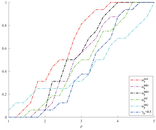
Figure 1. Comparison of six methods on CPU time for Example 1.

Example 2. 

Consider the following optimization problem,

$$\underset{x\in R^3}{\min }f\left(x\right)={\displaystyle \frac{1}{2}}{x}^T\left[\begin{array}{ccc}a& & \\ & a& \\ & & b\end{array}\right]x,$$

(72)

where $0<a<b$, initial point $x_0={(9,6,2)}^T$, $ϵ={10}^{-6}$.

For Example 2, we give the comparison results of the number of iterations and the minimum points of each method when solving the optimization problems with different values of a and b in Table 2. And we give a comparison of the CPU time of different methods when solving Example 2 in Figure 2.

Table 2. Number of iterations and minimum points of compared methods for Example 2.

$a,b$	${\alpha }_k^{new}$	${\alpha }_k^{BB1}$	${\alpha }_k^{BB2}$
	iter ($x^{*}$)	iter ($x^{*}$)	iter ($x^{*}$)
$a=2,b=5$	7 ${(1.93e-5,1.28e-5,0.0002)}^T$	7 ${(4.79e-5,3.19e-5,0.0002)}^T$	7 ${(2.89e-6,1.92e-6,8.78e-5)}^T$
$a=10,b=16$	7 ${(1.57e-9,1.04e-9,6.55e-8)}^T$	7 ${(2.79e-9,1.86e-9,8.09e-8)}^T$	7 ${(6.73e-10,4.49e-10,5.00e-8)}^T$
$a=25,b=30$	5 ${(2.08e-5,1.39e-5,9.42e-9)}^T$	5 ${(2.08e-5,1.38e-5,1.12e-8)}^T$	5 ${(2.09e-5,1.39e-5,7.81e-9)}^T$
$a=50,b=120$	7 ${(9.10e-6,6.07e-6,8.78e-5)}^T$	7 ${(2.21e-5,1.47e-5,0.0001)}^T$	7 ${(1.51e-6,1.01e-6,5.00e-5)}^T$
$a=100,b=350$	10 ${(1.18e-5,7.84e-6,-1.13e-11)}^T$	10 ${(3.99e-5,2.67e-5,-6.16e-10)}^T$	9 ${(3.46e-7,2.31e-7,1.16e-6)}^T$
$a=1000,b=5000$	14 ${(3.98e-10,2.65e-10,-1.90e-7)}^T$	15 ${(2.68e-5,1.79e-5,4.35e-9)}^T$	12 ${(3.76e-17,2.51e-17,-4.77e-10)}^T$
a = 10,000, b = 15,000	7 ${(2.89e-10,1.93e-10,1.51e-8)}^T$	7 ${(4.83e-10,3.22e-10,1.81e-8)}^T$	7 ${(1.42e-10,9.46e-11,1.20e-8)}^T$
$a,b$	${\alpha }_k^{DY}$	${\gamma }_k=0.5$	${\alpha }_k^{MG}$
	iter ($x^{*}$)	iter ($x^{*}$)	iter ($x^{*}$)
$a=2,b=5$	7 ${(1.92e-5,1.20e-5,0.0001)}^T$	7 ${(1.95e-5,1.30e-5,0.0002)}^T$	12 ${(0.0004,0.0003,-0.0002)}^T$
$a=10,b=16$	7 ${(1.70e-9,1.11e-9,6.55e-8)}^T$	7 ${(1.57e-9,1.05e-9,6.55e-8)}^T$	7 ${(0.0001,7.96e-5,2.65e-5)}^T$
$a=25,b=30$	5 ${(2.08e-5,1.30e-5,9.50e-5)}^T$	5 ${(2.08e-5,1.38e-5,9.42e-9)}^T$	5 ${(2.76e-5,1.84e-5,6.14e-6)}^T$
$a=50,b=120$	7 ${(9.09e-6,6.08e-6,8.80e-5)}^T$	7 ${(9.21e-6,6.14e-6,8.82e-5)}^T$	13 ${(0.0001,7.14e-5,2.38e-5)}^T$
$a=100,b=350$	10 ${(1.11e-5,7.88e-6,-1.15e-11)}^T$	10 ${(1.30e-5,8.68e-6,-1.43e-11)}^T$	20 ${(0.0001,7.26e-5,-1.65e-5)}^T$
$a=1000,b=5000$	14 ${(4.00e-10,2.65e-10,-1.90e-7)}^T$	14 ${(1.04e-9,6.93e-10,-2.70e-7)}^T$	23 ${(4.49e-5,3.00e-5,9.99e-6)}^T$
a = 10,000, b = 15,000	7 ${(2.80e-10,1.93e-10,1.50e-8)}^T$	7 ${(2.90e-10,1.93e-10,1.51e-8)}^T$	8 ${(1.56e-6,1.04e-6,-3.01e-6)}^T$

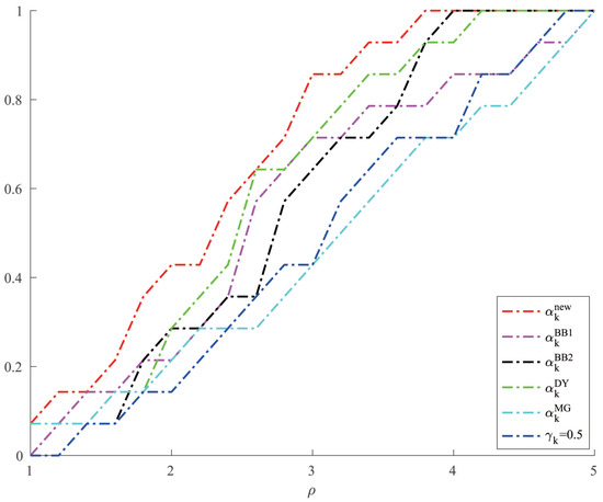
Figure 2. Comparison of six methods on CPU time for Example 2.

Example 3. 

Consider the following optimization problem,

$$\underset{x\in R^3}{\min }f\left(x\right)={\displaystyle \frac{1}{2}}{x}^T\left[\begin{array}{ccc}1& 0& 0\\ 0& \lambda & 0\\ 0& 1& \lambda \end{array}\right]x,$$

(73)

where $\lambda >1$, $ϵ={10}^{-8}$ and the initial point $x_0\in R^3$ can be chosen at random.

For Example 3, due to the particularity of its form, A is not a symmetric matrix but other forms of BB methods require A to be a symmetric positive definite matrix. Therefore, we only give the results of the number of iterations and the minimum points of this kind of optimization problems by using the new method when the initial points change in Table 3.

Table 3. Number of iterations and minimum points of our method for Example 3.

$\lambda$	${(-2,2,1)}^T$	${(1,2,0)}^T$	${(-1,-2,1)}^T$
	iter ($x^{*}$)	iter ($x^{*}$)	iter ($x^{*}$)
3	11 ${(-0.0001,5.56e-6,4.09e-6)}^T$	10 ${(2.69e-6,-6.88e-7,6.57e-7)}^T$	11 ${(-8.69e-7,-3.00e-6,-1.29e-6)}^T$
5	14 ${(-2.46e-7,-1.64e-6,-2.08e-6)}^T$	14 ${(5.38e-7,-1.47e-6,-1.62e-6)}^T$	10 ${(-0.0002,1.73e-5,-1.54e-5)}^T$
10	11 ${(-5.39e-6,2.85e-6,2.91e-6)}^T$	14 ${(3.01e-7,-9.89e-6,-4.34e-6)}^T$	12 ${(-7.13e-9,2.04e-5,-2.02e-5)}^T$
50	13 ${(-1.46e-5,4.94e-8,5.23e-8)}^T$	14 ${(2.88e-7,1.56e-6,-2.01e-6)}^T$	13 ${(-2.20e-6,-1.72e-8,-1.64e-8)}^T$
100	13 ${(-4.42e-6,2.84e-8,-2.33e-8)}^T$	14 ${(5.92e-7,1.57e-6,-4.91e-6)}^T$	13 ${(-3.87e-6,-8.53e-9,-3.62e-9)}^T$
500	13 ${(-3.44e-7,4.65e-9,-4.60e-9)}^T$	9 ${(0.0022,2.75e-8,-6.26e-10)}^T$	13 ${(-5.49e-6,-9.12e-9,7.72e-9)}^T$
1000	13 ${(-1.86e-7,1.53e-9,-1.52e-9)}^T$	9 ${(0.0022,6.86e-9,-7.83e-11)}^T$	13 ${(-5.72e-6,-1.00e-8,9.38e-9)}^T$
10,000	13 ${(-8.86e-8,9.85e-14,3.86e-12)}^T$	8 ${(0.0022,-1.17e-10,-1.37e-6)}^T$	13 ${(-5.93e-6,-1.10e-8,1.10e-8)}^T$
$\lambda$	${(3,2,1)}^T$	${(9,7,0)}^T$
	iter ($x^{*}$)	iter ($x^{*}$)
3	11 ${(2.57e-5,-5.13e-6,7.03e-6)}^T$	12 ${(3.33e-9,-3.17e-5,-1.54e-5)}^T$
5	14 ${(2.44e-6,-5.61e-6,-6.03e-6)}^T$	13 ${(1.06e-5,2.10e-5,2.19e-5)}^T$
10	14 ${(2.98e-7,-2.91e-6,-3.93e-6)}^T$	14 ${(1.76e-6,-2.42e-5,-1.14e-5)}^T$
50	13 ${(2.40e-8,-2.32e-8,4.86e-8)}^T$	14 ${(2.59e-5,-7.07e-6,-1.86e-6)}^T$
100	13 ${(1.77e-6,-1.35e-8,4.00e-8)}^T$	14 ${(1.72e-5,-2.84e-7,-1.33e-7)}^T$
500	13 ${(6.29e-7,7.88e-9,-7.76e-9)}^T$	13 ${(1.33e-7,3.19e-7,3.65e-7)}^T$
1000	13 ${(1.59e-7,4.25e-9,-4.23e-9)}^T$	13 ${(2.08e-6,6.67e-7,8.73e-7)}^T$
10,000	8 ${(0.0093,-1.90e-9,-2.01e-9)}^T$	8 ${(0.0089,-6.99e-9,-2.14e-7)}^T$

Example 4. 

Consider the following optimization problem,

$$\underset{x\in R^n}{\min }f\left(x\right)={\displaystyle \frac{1}{2}}{x}^T\left[\begin{array}{cccc}{\lambda }_1& & & \\ & {\lambda }_2& & \\ & & \ddots & \\ & & & {\lambda }_n\end{array}\right]x,$$

(74)

where $n=100$, $1\le {\lambda }_1\le {\lambda }_2\le \cdots \le {\lambda }_n$, $ϵ={10}^{-8}$ and the initial point $x_0\in R^n$ can be chosen at random.

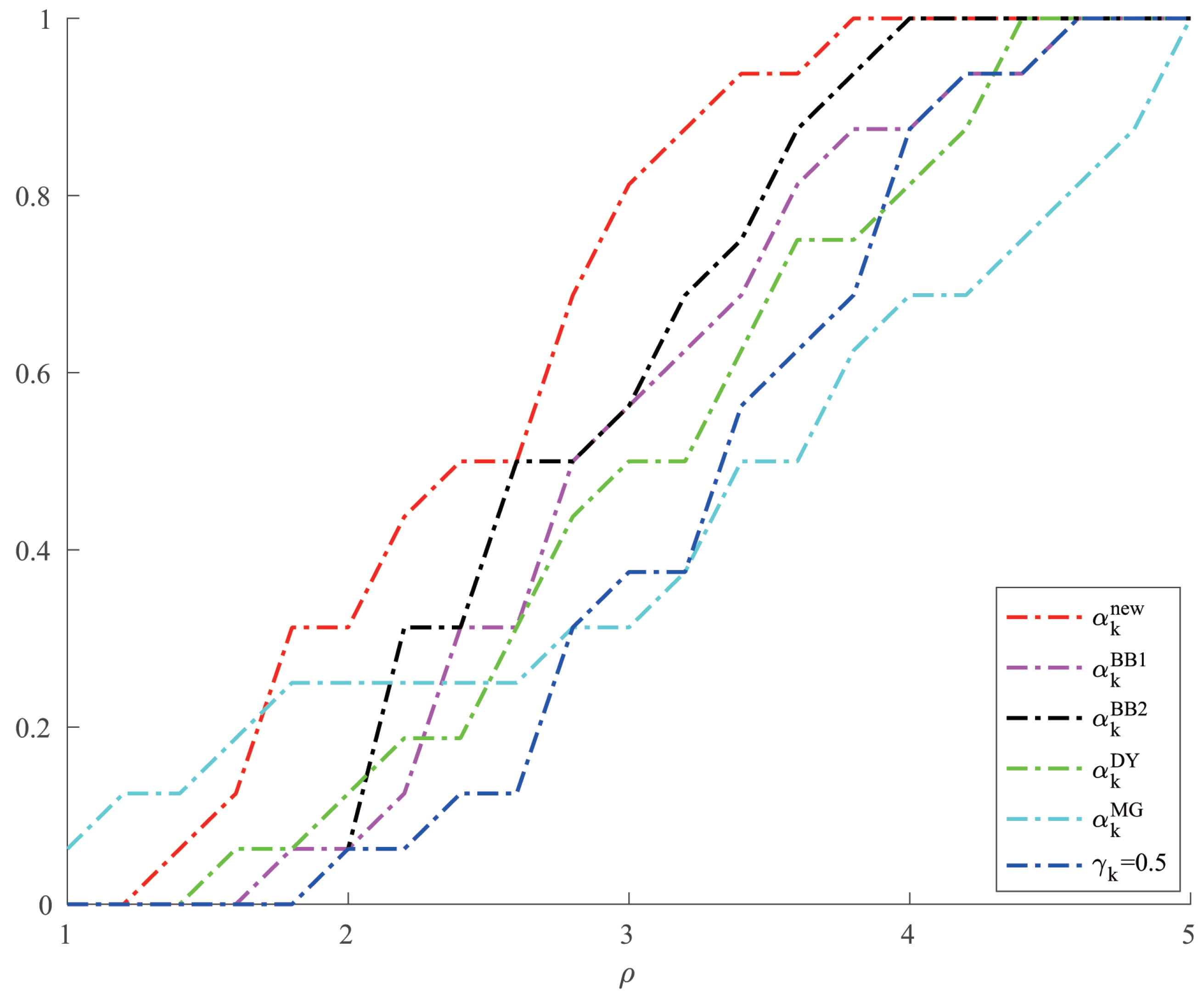
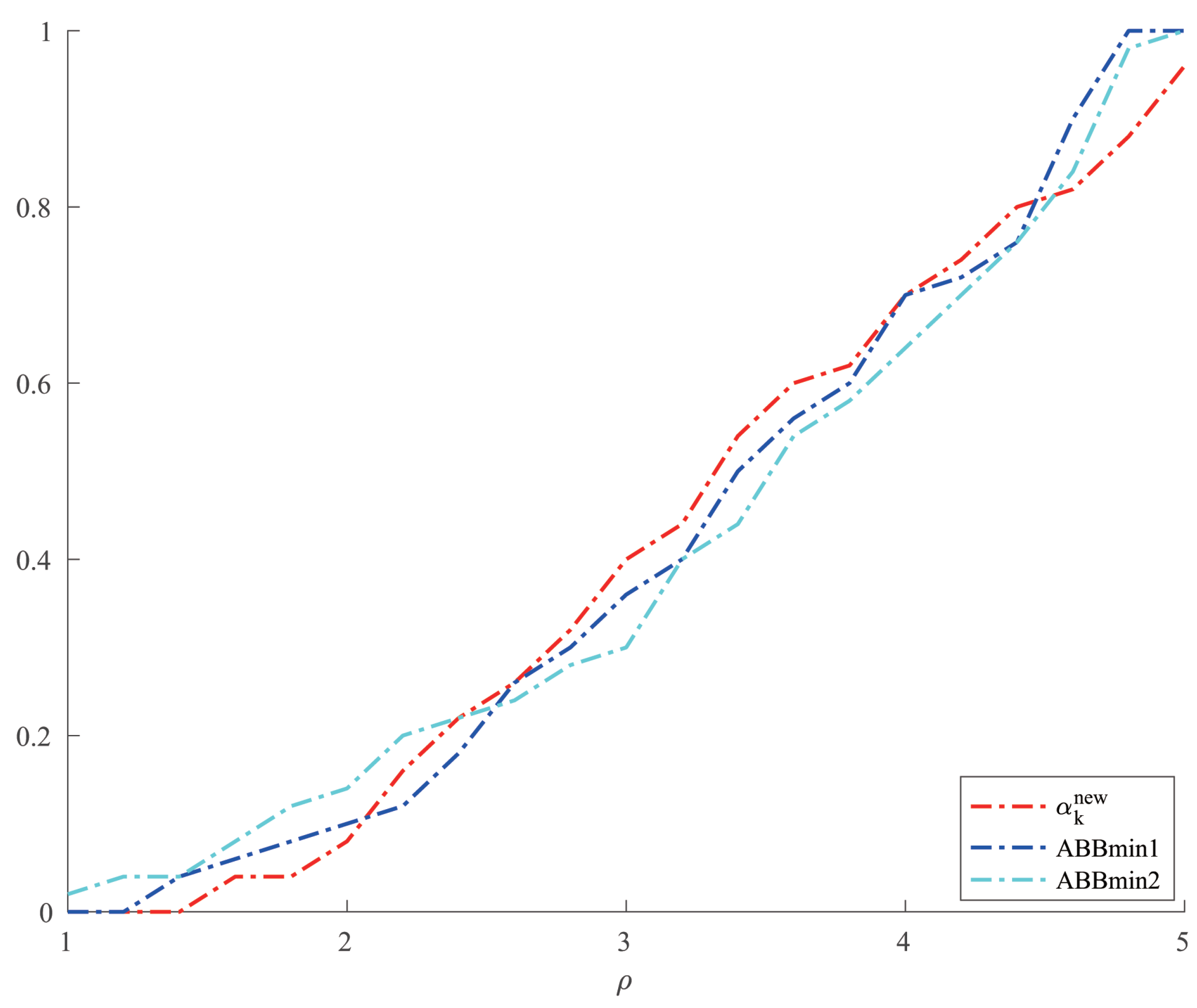
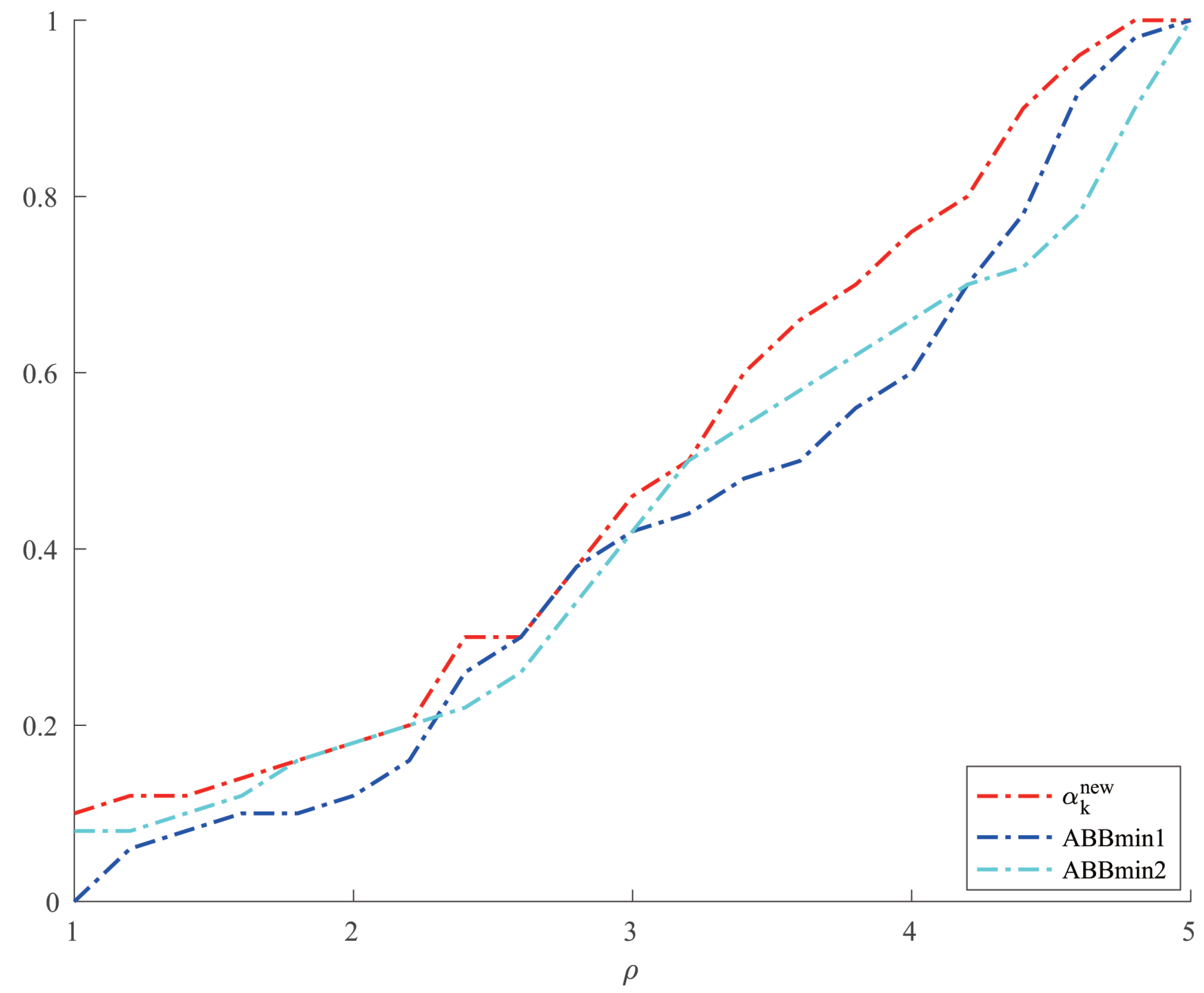
For Example 4, we chose two other methods, ABBmin1 and ABBmin2 methods, to compare with our method. The parameters of ABBmin1 and ABBmin2 methods were selected as in [18], which were $\tau =0.8$, $m=9$ and $\tau =0.9$, respectively. The initial points we chose were $(-10,5,2)$, $(-9,-7,-1)$ and $(7,3,5)$. For each initial point, we randomly chose ten different sets of values of ${\lambda }_i$, $i=1,\cdots ,100$, which satisfied ${\lambda }_1=1$, ${\lambda }_{100}=$ 10,000, and ${\lambda }_j$ was evenly distributed between 1 and 10,000 for $j=2,\cdots ,99$. Figure 3 and Figure 4, respectively, show the results of the comparison of the number of iterations and the CPU time when the three methods solve Example 4.

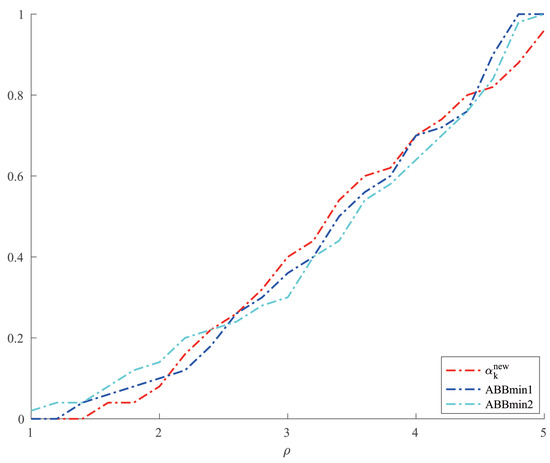
Figure 3. Comparison of three methods on number of iterations for Example 4.

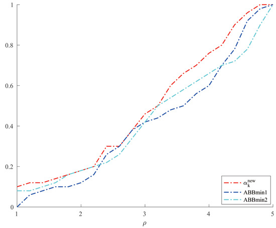
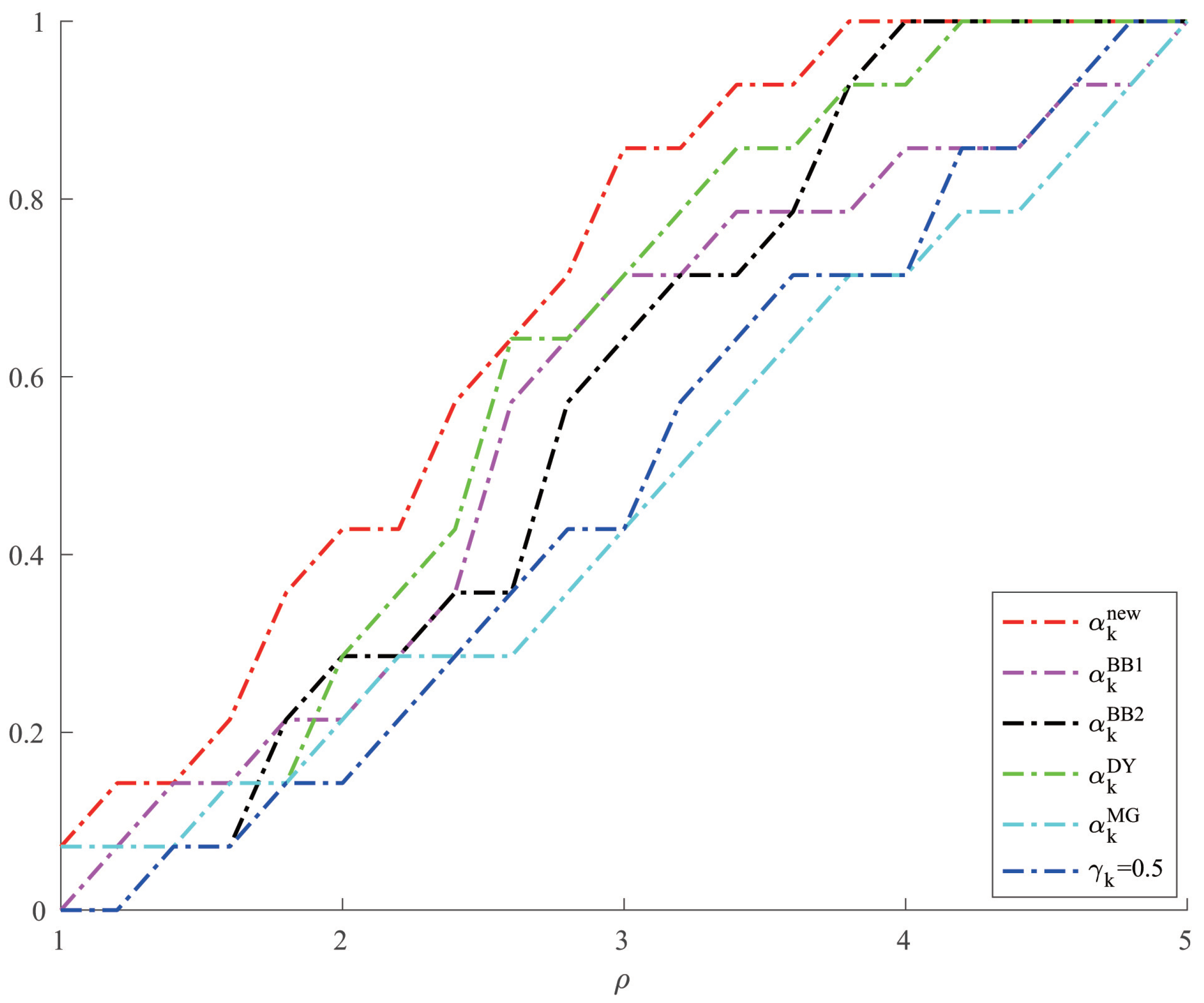
Figure 4. Comparison of three methods on CPU time for Example 4.

Example 5 

(Random problems in [33]). Consider $A=QD{Q}^T$, where

$$Q=(I-2{\omega }_3{\omega }_3^T)(I-2{\omega }_2{\omega }_2^T)(I-2{\omega }_1{\omega }_1^T),$$

and ${\omega }_1$, ${\omega }_2$, ${\omega }_3$ are unitary random vectors, $D=diag({\sigma }_1,\cdots ,{\sigma }_n)$ is a diagonal matrix where ${\sigma }_1=1$, ${\sigma }_n=cond$, and ${\sigma }_j$ is randomly generated between 1 and condition number $cond$ for $j=2,\cdots ,n-1$. We set $b=\mathbf{0}$, $ϵ={10}^{-8}$, and the initial point $x_0={(1,\cdots ,1)}^T$.

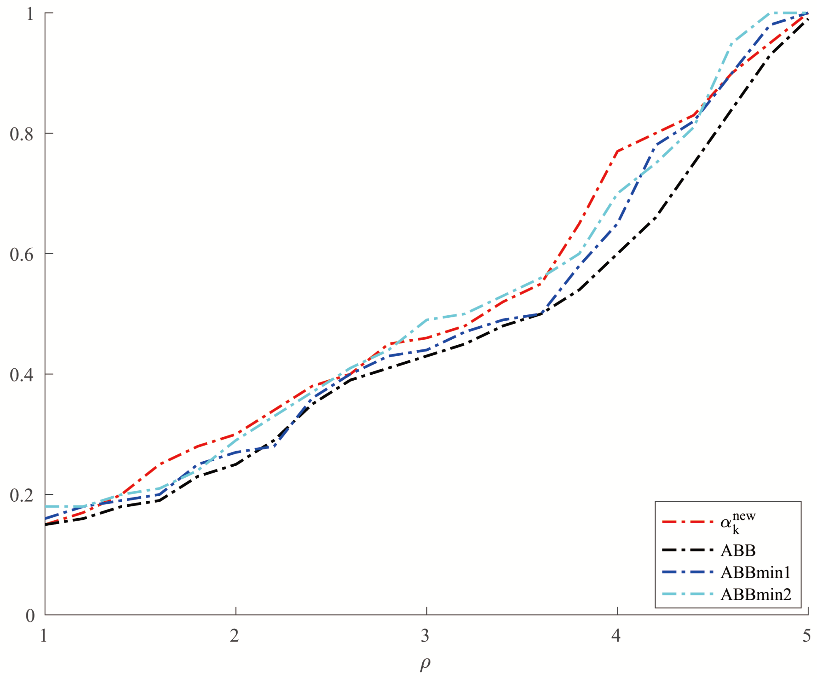
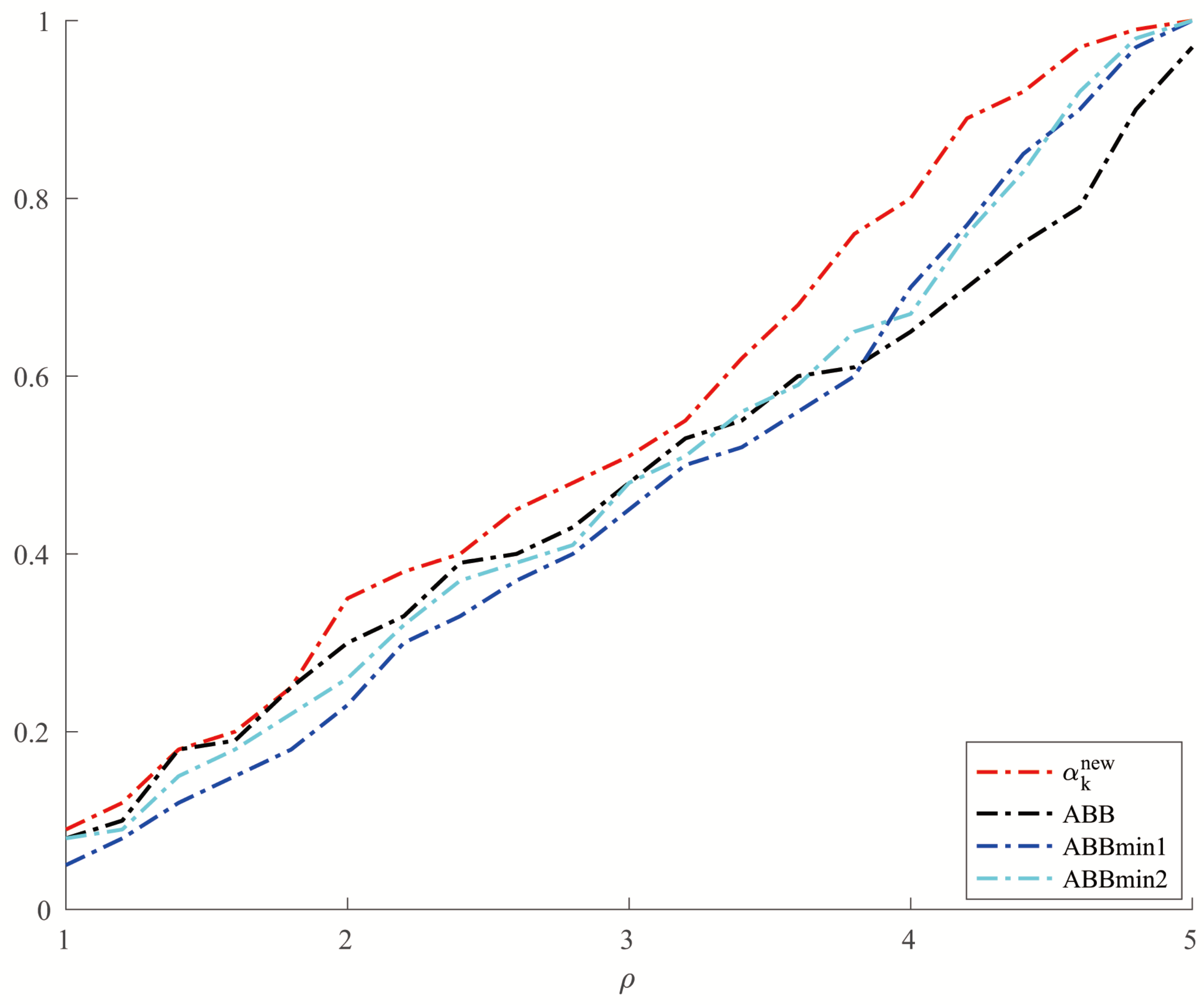
For Example 5, we set $n=2000$ and allowed a maximum of 10,000 iterations. In order to make a better comparison, we chose three other methods, which were ABBmin1 and ABBmin2 methods, and ABB method. The parameters used by the ABBmin1 and ABBmin2 methods were the same as Example 4. And for the ABB method, we set $\kappa =0.15$, which was different from that in [17]. In the experiments, three values of the condition number cond: ${10}^4,{10}^5,{10}^6$ were chosen. For each value of $cond$, ten instances with ${\sigma }_j$ evenly distributed in $[1,cond]$ were generated, $j=2,\cdots ,n-1$. The comparison of the number of iterations and the CPU time of several methods in solving Example 5 are shown in Figure 5 and Figure 6.

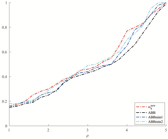
Figure 5. Comparison of four methods on number of iterations for Example 5.

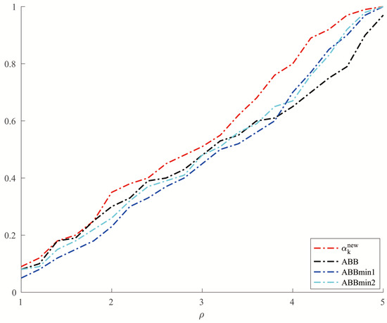
Figure 6. Comparison of four methods on CPU time for Example 5.

In all tables, ‘iter’ represents the number of iterations and ‘$x^{*}$’ represents the optimal solution. And the vertical axis of each figure shows the percentage of problems solved by different methods within the minimum value of the metric factor $\rho$.

From Table 1 and Table 2, we can see that the new method has no obvious advantage in the number of iterations when solving the optimization problems like Examples 1 and 2 and the solution accuracy can reach the level of other methods. However, in terms of CPU time, we can see from Figure 1 and Figure 2 that the new method has a clear advantage over other compared methods. When solving optimization problems like Example 3, it is not difficult to see from Table 3 that the new method can complete well in terms of the number of iterations and the accuracy of the minimum points. And from Figure 3 and Figure 4, we can see that there is no significant difference in the number of iterations between the three methods when solving the problems such as Example 4, but the new method has a slight advantage in terms of the CPU time. For the random problems like Example 5, we can see from Figure 5 that the new method and ABBmin2 method perform better in terms of the number of iterations, while in terms of the CPU time, we can see from Figure 6 that the new method still has obvious advantages.

5. Conclusions

In this paper, we proposed a modified BB-like method which used the stepsize ${\alpha }_k^{new}$ and analyzed two cases when the the coefficient matrix A of the quadratic term of quadratic function is a three-order matrix. For the case, $A=\left[\begin{array}{ccc}1& & \\ & 1& \\ & & \lambda \end{array}\right],\lambda >1$, we have proved the R-superlinear convergence of this case and generalized this case to $A=\left[\begin{array}{ccc}\mu & & \\ & \mu & \\ & & \phi \end{array}\right]$, $\phi >\mu \ge 1$. In addition to that, we have further generalized this case to the n-dimensional form, that is, $A=\mathrm{diag}\{{\lambda }_1,{\lambda }_2,\cdots ,{\lambda }_n\}$, where $1={\lambda }_1\le {\lambda }_2\le \cdots \le {\lambda }_n$. And we have proved the R-linear convergence of the n-dimensional case. The numerical experimental results have shown that this method has significant advantage in running time when comparing with some other methods. For another case $A=\left[\begin{array}{ccc}1& 0& 0\\ 0& \lambda & 0\\ 0& 1& \lambda \end{array}\right]$, $\lambda >1$, we also proved the global convergence of this case under some assumption and by the numerical results we can see that this modified method is fast and effective in dealing with problems. To sum up, using the modified stepsize ${\alpha }_k^{new}$ to solve three-dimensional optimization problems is well-behaved.

References

- Cauchy, A. Méthode générale pour la résolution des systemes d’équations simultanées. Comp. Rend. Sci. Paris 1847, 25, 536–538. [Google Scholar]
- Forsythe, G.E. On the asymptotic directions of the s-dimensional optimum gradient method. Numer. Math. 1968, 11, 57–76. [Google Scholar] [CrossRef]
- Nocedal, J.; Sartenaer, A.; Zhu, C. On the behavior of the gradient norm in the steepest descent method. Comput. Optim. Appl. 2002, 22, 5–35. [Google Scholar] [CrossRef]
- Barzilai, J.; Borwein, J.M. Two-point step size gradient methods. IMA J. Numer. Anal. 1988, 8, 141–148. [Google Scholar] [CrossRef]
- Dennis, J.E., Jr.; Moré, J.J. Quasi-Newton methods, motivation and theory. SIAM Rev. 1977, 19, 46–89. [Google Scholar] [CrossRef]
- Birgin, E.G.; Martínez, J.M.; Raydan, M. Spectral projected gradient methods: Review and perspectives. J. Stat. Softw. 2014, 60, 1–21. [Google Scholar] [CrossRef]
- Fletcher, R. On the Barzilai-Borwein method. In Optimization and Control with Applications; Qi, L.Q., Teo, K., Yang, X.Q., Eds.; Springer: New York, NY, USA, 2005; pp. 235–256. [Google Scholar]
- Crisci, S.; Porta, F.; Ruggiero, V.; Zanni, L. Spectral properties of Barzilai-Borwein rules in solving singly linearly constrained optimization problems subject to lower and upper bounds. SIAM J. Optim. 2020, 30, 1300–1326. [Google Scholar] [CrossRef]
- Huang, Y.K.; Dai, Y.H.; Liu, X.W. Equipping the Barzilai-Borwein method with the two dimensional quadratic termination property. SIAM J. Optim. 2021, 31, 3068–3096. [Google Scholar] [CrossRef]
- Huang, Y.; Liu, H. On the rate of convergence of projected Barzilai-Borwein methods. Optim. Methods Softw. 2015, 30, 880–892. [Google Scholar] [CrossRef]
- Dai, Y.H.; Liao, L.Z. R-linear convergence of the Barzilai-Borwein gradient method. IMA J. Numer. Anal. 2002, 22, 1–10. [Google Scholar] [CrossRef]
- Raydan, M. The Barzilai and Borwein gradient method for the large scale unconstrained minimization problem. SIAM J. Optim. 1997, 7, 26–33. [Google Scholar] [CrossRef]
- Grippo, L.; Lampariello, F.; Lucidi, S. A nonmonotone line search technique for Newton’s method. SIAM J. Numer. Anal. 1986, 23, 707–716. [Google Scholar] [CrossRef]
- Dai, Y.H.; Fletcher, R. Projected Barzilai-Borwein methods for large-scale box-constrained quadratic programming. Numer. Math. 2005, 100, 21–47. [Google Scholar] [CrossRef]
- Huang, Y.; Liu, H. Smoothing projected Barzilai-Borwein method for constrained non-Lipschitz optimization. Comput. Optim. Appl. 2016, 65, 671–698. [Google Scholar] [CrossRef]
- Dai, Y.H. Alternate step gradient method. Optimization 2003, 52, 395–415. [Google Scholar] [CrossRef]
- Zhou, B.; Gao, L.; Dai, Y.H. Gradient methods with adaptive step-sizes. Comput. Optim. Appl. 2006, 35, 69–86. [Google Scholar] [CrossRef]
- Frassoldati, G.; Zanni, L.; Zanghirati, G. New adaptive stepsize selections in gradient methods. J. Ind. Manag. Optim. 2008, 4, 299–312. [Google Scholar] [CrossRef]
- De Asmundis, R.; Di Serafino, D.; Hager, W.W.; Toraldo, G.; Zhang, H. An efficient gradient method using the Yuan steplength. Comput. Optim. Appl. 2014, 59, 541–563. [Google Scholar] [CrossRef]
- Dai, Y.H.; Yuan, Y.X. Analysis of monotone gradient methods. J. Ind. Manag. Optim. 2005, 1, 181–192. [Google Scholar] [CrossRef]
- Broyden, C.G. A class of methods for solving nonlinear simultaneous equations. Math. Comput. 1965, 19, 577–593. [Google Scholar] [CrossRef]
- Davidon, W.C. Variable metric method for minimization. SIAM J. Optim. 1991, 1, 1–17. [Google Scholar] [CrossRef]
- Fletcher, R.; Powell, M.J.D. A rapidly convergent descent method for minimization. Comput. J. 1963, 6, 163–168. [Google Scholar] [CrossRef]
- Broyden, C.G. The convergence of single-rank quasi-Newton methods. Math. Comput. 1970, 24, 365–382. [Google Scholar] [CrossRef]
- Fletcher, R. A new approach to variable metric algorithms. Comput. J. 1970, 13, 317–322. [Google Scholar] [CrossRef]
- Goldfrab, D. A family of variable-metric methods derived by variational means. Math. Comput. 1970, 24, 23–26. [Google Scholar] [CrossRef]
- Shanno, D.F. Conditioning if quasi-Newton methods for function minimization. Math. Comput. 1970, 24, 647–656. [Google Scholar] [CrossRef]
- Dai, Y.H.; Huang, Y.; Liu, X.W. A family of spectral gradient methods for optimization. Comput. Optim. Appl. 2019, 74, 43–65. [Google Scholar] [CrossRef]
- Dai, Y.H.; Al-Baali, M.; Yang, X. A positive Barzilai-Borwein-like stepsize and an extension for symmetric linear systems. In Numerical Analysis and Optimization; Al-Baali, M., Grandientti, L., Purnama, A., Eds.; Springer: Cham, Switzerland, 2015; pp. 59–75. [Google Scholar]
- Dai, Y.H.; Yang, X.Q. A new gradient method with an optimal stepsize property. Comput. Optim. Appl. 2006, 33, 73–88. [Google Scholar] [CrossRef]
- Elman, H.C.; Golub, G.H. Inexact and preconditioned Uzawa algorithm for saddle point problems. SIAM J. Numer. Anal. 1994, 31, 1645–1661. [Google Scholar] [CrossRef]
- Dai, Y.H.; Yuan, Y.X. Alternate minimization gradient methods. IMA J. Numer. Anal. 2003, 23, 377–393. [Google Scholar] [CrossRef]
- Friedlander, A.; Martínez, J.M.; Molina, B.; Raydan, M. Gradient method with retards and generalizations. SIAM J. Numer. Anal. 1999, 36, 275–289. [Google Scholar] [CrossRef]
Disclaimer/Publisher’s Note: The statements, opinions and data contained in all publications are solely those of the individual author(s) and contributor(s) and not of MDPI and/or the editor(s). MDPI and/or the editor(s) disclaim responsibility for any injury to people or property resulting from any ideas, methods, instructions or products referred to in the content. |
© 2025 by the authors. Licensee MDPI, Basel, Switzerland. This article is an open access article distributed under the terms and conditions of the Creative Commons Attribution (CC BY) license (https://creativecommons.org/licenses/by/4.0/).