An Adaptive Large Neighborhood Search for a Green Vehicle Routing Problem with Depot Sharing

Abstract

In urban logistics distribution, vehicle carbon emissions during the distribution process significantly contribute to environmental pollution. While developing green logistics is critical for the sustainable growth of the logistics industry, existing studies often overlook the potential benefits of depot sharing among enterprises. By enabling depots belonging to different enterprises to be shared, it would shorten the distance traveled by vehicles returning to depots and reduce carbon emissions. And it would also reduce the number of depots being built. Therefore, a green vehicle routing problem with depot sharing is presented in the paper. To solve this problem, an improved adaptive large neighborhood search algorithm is presented, in which the Split strategy and two new operators are proposed to enhance solution quality and computational efficiency. Extensive numerical experiments are conducted on instances of varying scales to evaluate this algorithm, and also demonstrate its effectiveness and efficiency. Furthermore, the experimental results demonstrate that depot sharing significantly reduces carbon emissions, achieving an average optimization rate of 10.1% across all instances compared to returning to the original depot.

1. Introduction

In the past decade, global warming has been a hot topic and has aroused more and more concern. Several recent studies [1] have demonstrated the seriousness of global warming. One of the main causes of global warming is the large amount of greenhouse gases produced by human activities, of which carbon dioxide is the main component. The global transport network generates a significant amount of carbon emissions, with road transport responsible for approximately 75% of this total [2]. It can be seen that most carbon emissions are generated during supply chain logistics and distribution. In 2020, China introduced robust policies and measures aimed at reaching peak carbon emissions by 2030 and achieving carbon neutrality by 2060 [3]. Therefore, the green vehicle routing problem (GVRP) is a variant of the traditional vehicle routing problem (VRP), which is receiving more and more attention from governments [4]. GVRP is a comprehensive optimization problem that integrates environmental objectives with traditional routing considerations, as highlighted in recent research [5].

With the continuous expansion of the scale of logistics enterprises, supply chain networks increasingly involve multiple depots and numerous delivery points. Therefore, multi-depot logistics distribution has become prevalent [6], highlighting the practical importance of minimizing carbon emissions in the multi-depot vehicle routing problem (MDVRP). In addition, in order to be closer to the real-life scenario, each customer has a time window. Therefore, the multi-depot green vehicle routing problem with time windows (MDGVRPTW) is an extension of GVRP. MDGVRPTW is considered to be an NP-Hard problem, which plans vehicles departing from multiple depots, passing through each set of delivery points, and finally returning to the depot, while not exceeding the capacity of the vehicle and must obey the time window constraints of each customer.

In order to solve this complex problem, this paper proposes an adaptive large neighborhood search (ALNS) algorithm, which has proven to be highly effective in vehicle routing [7]. Examples of its successful applications include the multi-depot open VRP(MDOVRP) [8], multi-compartment VRP(MCVRP) [9], multi-depot multi-compartment VRP(MDMCVRP) [9], and two-echelon VRP(2E-VRP) [10]. In addition, [11] proposed the Split strategy and introduced the application of Split in solving VRP in detail. And combined with the ALNS algorithm, this combination has advantages in improving algorithm performance, speeding up the search process and increasing the diversity of global search.

Despite the progress made in addressing GVRP, existing studies often focus on traditional VRP or GVRP, with limited attention given to multi-depot logistics scenarios involving depot sharing. Most of the research assumes that vehicles must return to their original depots, which can lead to inefficiencies in logistics operations and increased carbon emissions. Furthermore, the integration of depot-sharing strategies with environmental objectives has not been thoroughly investigated. this paper proposes a green vehicle routing problem with depot sharing (GVRPDS). Additionally, while ALNS algorithms have been widely applied in vehicle routing problems, their potential for solving GVRPDS remains underexplored. To address these gaps, this paper proposes a novel approach for the GVRP, introducing a depot-sharing strategy to minimize carbon emissions and enhance logistical efficiency. An improved ALNS algorithm is developed to solve the problem efficiently. This work makes the following contributions:

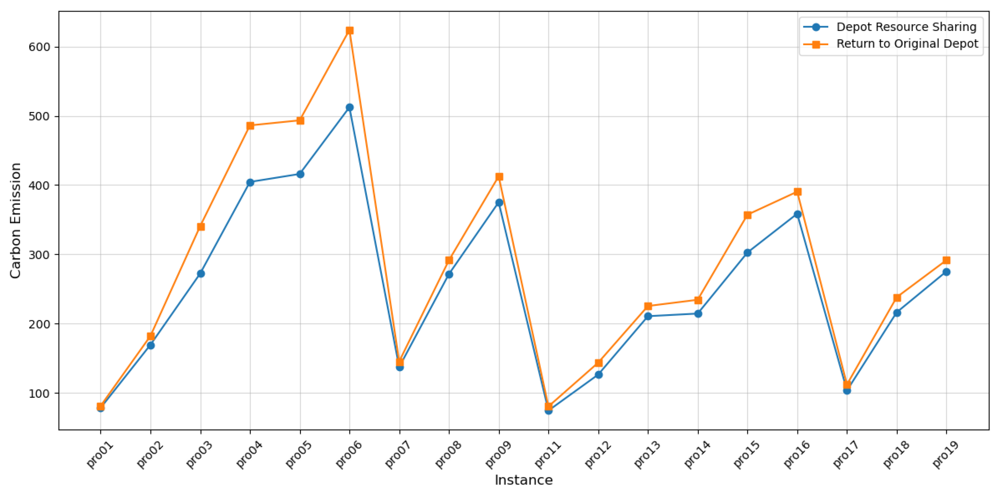
• The GVRPDS is presented in this manuscript, in which vehicles choose a nearby depot for return, thereby shortening the distance traveled by vehicles returning to depots and reducing carbon emissions.
• A carbon emission model of vehicle, which is positively correlated with fuel consumption based on vehicle load and distance, is established for calculating emissions during logistics distribution.
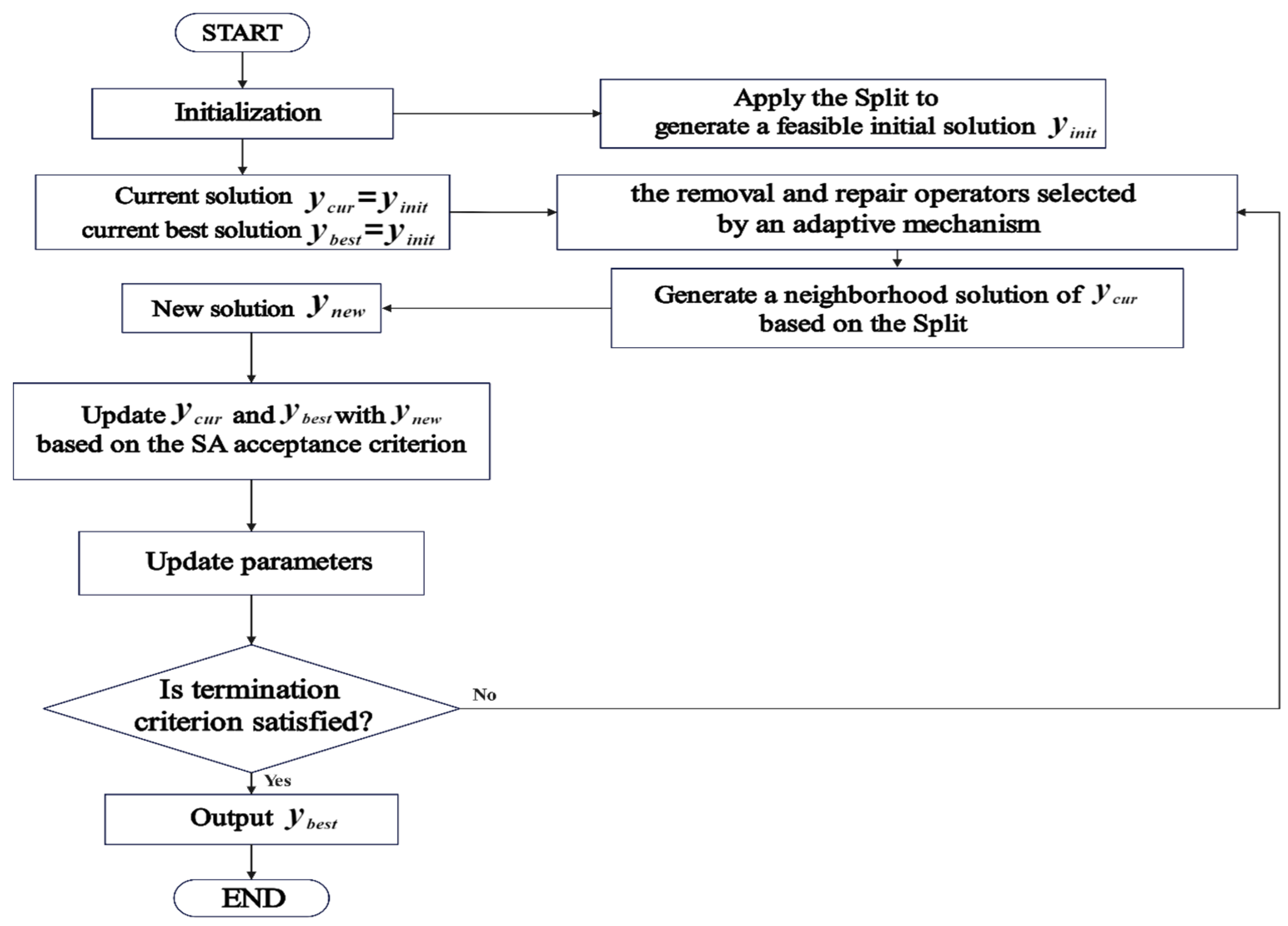
• An improved adaptive large neighborhood search algorithm is proposed to solve this GVRPDS, in which the Split strategy and two new operators are proposed to accelerate the convergence and to jump out of the local optimal solution.

The rest of the paper is structured as follows: In Section 2, the related literature is introduced and summarized. In Section 3, the description and formulation of GVRPDS are introduced. In Section 4, the improved ALNS algorithm is introduced. In Section 5, instances are used to validate the proposed method, and the corresponding results are analyzed in detail. Finally, we present our conclusions and outline some suggestions for future work in Section 6.

2. Literature Review

The GVRP has attracted significant research interest due to growing environmental awareness. According to the literature survey by Lin et al. [12], the GVRP can be categorized into three main types: the pollution routing problem (PRP), the green vehicle routing problem (G-VRP), and the energy minimization vehicle routing problem (EMVRP). PRP was proposed by Bektaş and Laporte [13], and it focuses on minimizing the environmental impact of greenhouse gases (GHG), especially carbon emissions in transport routes. Many researchers have highlighted vehicle distance and weight as important factors impacting carbon emissions [14]. In order to solve this problem, Rezaei et al. [15] proposed a hybrid integer linear programming model that considers vehicle type, load, and distance in fuel consumption, with a solution approach based on genetic algorithms and simulated annealing. Schneider et al. [16] studied the utilization of electric vehicle fleets in a green vehicle environment and introduced the electric VRP with time windows (EVRPTW). Amiri et al. [17] proposed a bi-objective programming model to solve the GVRP, which aims to minimize the total transportation cost and greenhouse gas emissions by optimizing the routing of electric and conventional trucks. In order to minimize carbon emissions, the GVRP with time window (GVRPTW) based on branch-cut and price (BCP) algorithm was solved exactly [18]. In addition, Ghannadpour [19] introduced a novel EMVRP model incorporating time windows and customer priority, aiming to minimize not only total driving distance but also energy consumption. Notably, the PRP is a specific instance of the GVRP, featuring a more comprehensive objective function that accounts for GHG emissions, driving time, costs, and driving distance. In addition to traditional and green vehicle routing problem models, recent research has explored the application of crowdsourcing in vehicle routing problems, particularly in urban logistics. For instance, Lu et al. [20] proposed a crowdsourcing delivery optimization model to address uncertainties in delivery distance, income, and task volume, helping logistics companies reduce delivery costs while maintaining a high coverage rate. Similarly, Yang et al. [21] developed a novel decomposition heuristic to address large-scale urban crowdsourced shared-trip delivery problems, demonstrating significant cost reductions through the integration of shared personal vehicles into delivery networks. While these studies focus on crowdsourced delivery models, our research centers on depot sharing among established logistics providers. Nonetheless, the emphasis on resource sharing in both approaches underscores the importance of collaborative strategies in enhancing urban delivery efficiency and reducing environmental impact. The above studies for GVRP consider only one depot.

Since the larger solution space of the MDVRP is compared to the single-depot problem, the routes planned from each depot need to be calculated and compared; as the optimization of route combinations originating from different depots becomes more complex, the search space for algorithms expands, leading to a further decrease in execution efficiency. The MDVRP was first proposed by Cassidy and Bennett [22] and has become a key problem in the field of combinatorial optimization. Multi-depot logistics distribution is widely used in practice. The study by Montoya-Torres et al. shows that most researchers prefer to adopt heuristic or metaheuristic approaches to solve MDVRP. Yu et al. [23] transformed MDVRP into the problem of single library VRP (SVRP) by introducing a virtual library in the first step and then applying a modified ant colony optimization (ACO) to solve SVRP. Özger [24] proposed the multi-yard routing problem with time window, and considered heterogeneous fleets, using a variable neighborhood genetic algorithm to solve it. Considering the timeliness requirements of fresh food distribution, Fan et al. [25] introduced the MDOVRP tailored for fresh food logistics using a joint distribution model. They formulated an optimization model to minimize total distribution costs and proposed an enhanced ant colony optimization (ACO) algorithm to solve it. Schmidt et al. [26] address the time-varying fleet size and mixed multi-parking vehicle routing problem by proposing mathematical models and effective inequalities to improve urban logistics and service design and develop effective traffic and congestion policies. Soriano et al. [27] proposed the multi-yard vehicle distribution problem with profit fairness (MDVRP-PF) by adding a fairness objective function to the classical cost minimization function and using the ALNS to solve the problem. Salehi Sarbijan and Behnamian [28] formulated the risk-constrained multi-vehicle segment routing problem (RCMDVRP) using real-time traffic data, and studied and developed a bi-objective model and a goal programming model, and proposed two improved genetic algorithms to solve the problem. These studies primarily overlook carbon emissions, whereas the MDGVRP, a variant of the MDVRP, emphasizes minimizing total carbon emissions from vehicle operations to tackle increasing environmental concerns.

The MDGVRP was proposed by Jabir et al. [29]. They integrated both the traditional economic route costs and carbon emission costs. Their model aimed to achieve a balanced reduction in both economic expenses and environmental impacts. By combining the ant colony algorithm with variable domain search, they successfully solved the problem of large-scale instances. Shen et al. [30] proposed a low-carbon multi-station open vehicle routing problem, and combined the time window and low-carbon trading policy, and designed a two-stage algorithm to solve the model. Qin et al. [31] proposed a low-carbon simultaneous pickup and delivery vehicle routing problem model, aiming to minimize the total cost and consider the cost of carbon emissions. They also developed an optimization model for the cold chain transport vehicle routing problem, taking into account transport costs, customer satisfaction, and carbon emissions.

It is crucial to choose a metaheuristic suitable for the optimization task, and ALNS is very effective in solving VRP. ALNS applies multiple competing removal and repair operators with frequencies that match historical performance and excel at solving large-scale instances [32]. This approach is built on the large neighborhood search (LNS) algorithm introduced by Ropke and Pisinger [33] to solve the pickup and delivery problem (PDP). Because of its excellent performance, ALNS is widely applied to various variants of VRP. Chen et al. [34] used ALNS to solve dynamic VRP and demonstrated the advantages of ALNS over general VNS and improved LNS algorithms. R. Liu et al. [35] proposed an efficient ALNS for VRPTW with synchronous access, showing that ALNS is also satisfactory compared to the simulated annealing algorithm. Azi et al. [36] proposed an adaptive large neighborhood search method using the destruction reproduction principle for solving the vehicle routing problem with multiple routes. Gu et al. [37] proposed a heuristic method based on adaptive large neighborhood search for solving the commodity constrained Split delivery vehicle routing problem (C-SDVRP). Sacramento et al. [38] proposed an ALNS for solving VRP with up to 375 customers.

3. Description and Formulation of GVRPDS

3.1. Problem Description

GVRPDS is classified as an NP-hard problem. It aims to minimize carbon emissions by determining optimal routes for multiple vehicles from various depots to a set of delivery points, while ensuring that vehicles return to the depot. The solution must also respect the capacity limits of each vehicle and adhere to time window constraints for each customer. $V=\{1,2,\dots ,n+m\}$ represents the vertex set, which consists of both customer nodes and depot nodes. Specifically, $C=\{1,2,\dots ,n\}$ represents the set of customers. $D=\{n,n+1,\dots ,n+m\}$ represents the set of depots. The locations of the depots, the capacities of the vehicles, and the customer information are all known. Usually, the vehicle needs to return to the original depot after serving the last customer. But the last customer is sometimes far away from the depot, and apparently returning to the original depot will increase the total driving distance and lead to more carbon emissions and pollution. And the vehicle is better to choose to return to the nearest depot. To clarify the application scope of this study, the following assumptions are made: (1) Vehicles must depart from the depot and return to the depot after completing their tasks. The speed is fixed. (2) The demand of each customer is less than the vehicle capacity. (3) The weight of the goods carried by each vehicle does not exceed its capacity. (4) Each customer is served only once by a single vehicle, and each customer requires a service time. (5) The number of vehicles returning to a depot cannot exceed the available parking spaces at the depot.

3.2. Mathematical Model

This section describes the definitions of some sets, parameters, and variables used in the mathematical model, as shown in

Table 1. Nomenclature of sets node, vehicle parameters, and variables.

Notation	Meaning
Sets $D$ $C$ $V$ $K$ Nodes parameters $q_i$ $e_i$ $l_i$ $t_i$ $P_d$ $K_d$ $Q_k$ $d_{ij}$ $q_{ij}$ Vehicle parameters $\omega$ $E_f$ $O$ $V$ $C_r$ $C_d$ $g$ $\theta$ $A$ $\rho$ ${\eta }_{tf}$ $\eta$ $\tau$ $\xi$ $\psi$ $\kappa$ Variables $x_{kij}$ $s_{ki}$ $t_{ij}$	The depot set The customer set The vertex set The vehicle set $\mathrm{Demand} \mathrm{of} \mathrm{customer} i$ $\mathrm{Customer} i$ earliest service time $\mathrm{Customer} i$ latest service time $\mathrm{Delivery} \mathrm{time} \mathrm{of} \mathrm{customer} i$ Depot D parking space capacity Number of vehicles in depot D The capacity of the vehicle k $\mathrm{Distance} \mathrm{from} \mathrm{customer} i$$\mathrm{to} \mathrm{customer} j$ $\mathrm{Load} \mathrm{of} \mathrm{vehicle} \mathrm{from} \mathrm{customer} i$$\mathrm{to} \mathrm{customer} j$ $\mathrm{The} \mathrm{vehicle} \mathrm{curb} \mathrm{weight} (\mathrm{Unit}\text{:} \mathrm{kg}$) $\mathrm{The} \mathrm{engine} \mathrm{friction} \mathrm{factor} (\mathrm{Unit}\text{:} \mathrm{rev}/\mathrm{L}$) $\mathrm{The} \mathrm{engine} \mathrm{speed} (\mathrm{Unit}\text{:} \mathrm{rev}/\mathrm{s}$) $\mathrm{The} \mathrm{engine} \mathrm{displacement} (\mathrm{Unit}\text{:} \mathrm{L}$) The rolling resistance coefficient The aerodynamic drag coefficient $\mathrm{The} \mathrm{gravitational} \mathrm{constant} (\mathrm{Unit}\text{:} \mathrm{m}/{\mathrm{s}}^2$) Road angle $\mathrm{The} \mathrm{vehicle} \mathrm{frontal} \mathrm{surface} \mathrm{area} (\mathrm{Unit}\text{:}{ \mathrm{m}}^2$) $\mathrm{The} \mathrm{air} \mathrm{density} (\mathrm{Unit}\text{:} \mathrm{kg}/{\mathrm{m}}^3$) The efficiency of the vehicle drive train The efficiency for diesel engines $\mathrm{The} \mathrm{instantaneous} \mathrm{acceleration} (\mathrm{Unit}\text{:} \mathrm{m}/{\mathrm{s}}^2$) The fuel-to-air mass ratio $\mathrm{The} \mathrm{conversion} \mathrm{factor} \mathrm{of} \mathrm{fuel} \mathrm{from} g/s$$\mathrm{to} l/s$ $\mathrm{The} \mathrm{heating} \mathrm{value} \mathrm{of} \mathrm{a} \mathrm{diesel} \mathrm{fuel} (\mathrm{Unit}\text{:} \mathrm{kj}/\mathrm{g}$) $\mathrm{Binary} \mathrm{variable} \mathrm{equal} \mathrm{to} 1 \mathrm{if} \mathrm{vehicle} \mathrm{k} \mathrm{is} \mathrm{used} \mathrm{to} \mathrm{connect} \mathrm{nodes} \mathrm{on} \mathrm{arc}\left(i,j\right)$, 0 otherwise $\mathrm{Time} \mathrm{when} \mathrm{vehicle} \mathrm{k} \mathrm{arrives} \mathrm{at} \mathrm{node} i$ $\mathrm{Travel} \mathrm{time} \mathrm{of} \mathrm{vehicle} \mathrm{k} \mathrm{from} \mathrm{node} i$$\mathrm{to} j$	Values 5000 0.2 36.67 6.9 0.01 0.7 9.81 0 8.0 1.20 0.45 0.45 0 1:14.7 737 4.4

. The vehicle parameter values were sourced from Koç et al. [39].

3.2.1. Carbon Emission Evaluation

Generally, the calculation of carbon dioxide emissions is based on fuel consumption and the corresponding emission coefficient. Here, the comprehensive modal emissions model (CMEM) is used to estimate fuel consumption, which was proposed by Scora and Barth [40]. It has been widely adopted to estimate fuel consumption and emissions for fuel-powered vehicles in the GVRP [41,42].

According to CMEM, the fuel consumption of a vehicle traveling at speed $v$ for a distance $d$ is given by

$$F=\lambda d\left\{{\displaystyle \frac{E_{f}OV}{v}}+\alpha \left[\beta M+\phi v^2\right]\right\}$$

(1)

where $\lambda =\xi /\left(\kappa \psi \right)$ represents the engine efficiency-related factor, $\alpha =1/\left(1000{\eta }_{tf}\eta \right)$ represents the fuel consumption coefficient, $\beta =\tau +g\sin \theta +g{C}_r\cos \theta$ represents the vehicle dynamics factor and $\phi =0.5C_{d}A\rho$ represents the air resistance-related factor, $M=\omega +q$ denotes the sum of the vehicles curb weight and the load weight. Table 1 is a list of parameters and their typical values.

According to the research, the amount of carbon dioxide emitted by cars is directly proportional to the fuel consumption. The calculation formula of carbon dioxide emission is as follows: $E=e\ast F$, where $e$ is the carbon dioxide emission during driving, $F$ is the fuel consumption during driving, and $E$ is the conversion factor of fuel carbon emission. According to the European carbon emission standard: $e=2.62kg/l$. In this way, the expression of the carbon emission of the vehicle within the driving arc $(i,j)$ is

$$E_{ij}=e\lambda d_{ij}\left\{{\displaystyle \frac{E_{f}OV}{v_{ij}}}+\alpha \left[\beta \left(\omega +q_{ij}\right)+\phi {\left(v_{ij}\right)}^2\right]\right\}$$

(2)

3.2.2. Optimization Model Formulation

We establish the GVRPDS as a mixed integer programming model and take the carbon emission as the objective function in this paper. The formula of GVRPDS is as follows:

$$\min Z={\displaystyle \sum _{(i,j)\in V}{\displaystyle \sum _{k\in K}{E}_{ij}{x}_{kij}}}$$

(3)

subject to

$${\displaystyle {\sum }_{j\in C}{\displaystyle {\sum }_{k\in K}{x}_{kdj}}}\le K_d,\forall d\in D$$

(4)

$${\displaystyle {\sum }_{(i,j)\in V}{\displaystyle {\sum }_{k\in K}{x}_{kij}}}={\displaystyle {\sum }_{(i,j)\in V}{\displaystyle {\sum }_{k\in K}{x}_{kji}}}=1$$

(5)

$${\displaystyle {\sum }_{d\in D}{\displaystyle {\sum }_{j\in C}{x}_{kdj}}}={\displaystyle {\sum }_{d\in D}{\displaystyle {\sum }_{i\in C}{x}_{kid}}}\le 1,\forall k\in K$$

(6)

$${\displaystyle {\sum }_{i\in D}{\displaystyle {\sum }_{j\in D}{x}_{kij}}}=0,\forall k\in K$$

(7)

$$N\le {\displaystyle {\sum }_{j\in C}{\displaystyle {\sum }_{k\in K}{x}_{kjd}}}\le P_d,\forall d\in D$$

(8)

$${\displaystyle {\sum }_{j\in C}{\displaystyle {\sum }_{i\in V}{x}_{kij}{q}_i}}\le Q_k,\forall k\in K$$

(9)

$$s_{ki}+t_{ij}-M(1-x_{kij})\le s_{jk},\forall (i,j)\in C,\forall k\in K$$

(10)

$$e_i\le s_{ki}\le l_i,i\in C,\forall k\in K$$

(11)

$$x_{kij}\in \left\{0,1\right\},\forall \left(i,j\right)\in V,\forall k\in K$$

(12)

In the mathematical formulation, Equation (3) represents the objective function, which aims to minimize the total carbon emission. Constraint (4) requires that the number of vehicles departing from each depot is not greater than the number of available vehicles. This is achieved by limiting the total number of departing vehicles at each depot to ensure reasonable allocation and use of resources. Constraint (5) ensures that each customer must be visited once by exactly one vehicle. By ensuring that the total number of visits of each customer is equal to 1, the comprehensiveness and efficiency of the service are ensured. Constraint (6) means that each vehicle starts at one depot and ends at one depot. Constraint (7) states that vehicles go directly from one depot to another. Constraint (8) requires that the number of vehicles returned to each depot is no more than the number of available parking Spaces and no less than $N$, ensuring that each depot has available cars. Constraint (9) ensures that the total demand of customers served by vehicle k is less than the maximum load of vehicle. Constraint (10) ensures the connectivity of the solution by introducing a large constant $M$ and decision variable $x_{ij}$, preventing the formation of subloop. Constraint (11) is guaranteed to be in the customer’s time window. Constraint (12) is the decision variable.

4. The Improved ALNS for the GVRPDS

ALNS is an extension of LNS, which solves the limitation of the LNS algorithm in a local search by introducing an adaptive mechanism. LNS relies on fixed removal and repair operators, which can easily lead the algorithm to fall into local optima in complex problems, and it is difficult to explore the whole solution space effectively. In contrast, ALNS enhances the flexibility and diversity of the search by introducing multiple removal and repair operators, allowing the algorithm to dynamically adjust the strategies used during the search process according to the effects of different operators. In the ALNS algorithm, the generation of the initial solution has a great influence on the quality of the final solution, and if the initial solution is not of high quality, more iterations may be needed to find a better solution. Due to the random destruction and repair operators of ALNS, the algorithm may fall into a local optimum and it is difficult to jump out of the local region. Prins et al. [11] proposed the path Split strategy. The ALNS algorithm combines the Split strategy, where the quality of the initial solution can be greatly improved. Such high-quality initial solutions can help the ALNS algorithm to find more potential solutions in the early stage and reduce the number of iterations. ALNS searches in the neighborhood through the removal–repair mechanism, although it can jump out of the local optimal solution, but sometimes the process of removal and repair may cause the search space to be limited to a certain area, affecting the diversity of solutions. After combining the Split, ALNS does not need to consider the constraint problem too much in the neighborhood search, focusing on the diversity and quality of solutions, and leaving the remaining constraints to the Split. In this way, more solutions with different structures can be introduced, which increases the diversity of the search space. Figure 1 shows the flowchart of the ALNS with the Split (SALNS).

The flowchart starts from the initialization phase and generates a feasible initial solution $y_{init}$ by applying the Split operation. Subsequently, the algorithm initializes the current solution $y_{cur}$ and the best solution $y_{best}$ to $y_{best}$. In the iterative process, the algorithm uses an adaptive mechanism to select removal and repair operations to generate a neighborhood solution $y_{new}$ based on the current solution $y_{cur}$. The new solution $y_{new}$ will be compared with the current solution according to the acceptance criterion of simulated annealing to decide whether to update the current solution and the best solution. In addition, the algorithm updates the relevant parameters after each iteration to adapt to the search process. The iterations continue until a termination criterion is met, such as a maximum number of iterations is reached or the quality of the solution is no longer significantly improved. Eventually, the algorithm outputs the best solution found so far, $y_{best}$ as the solution to the problem.

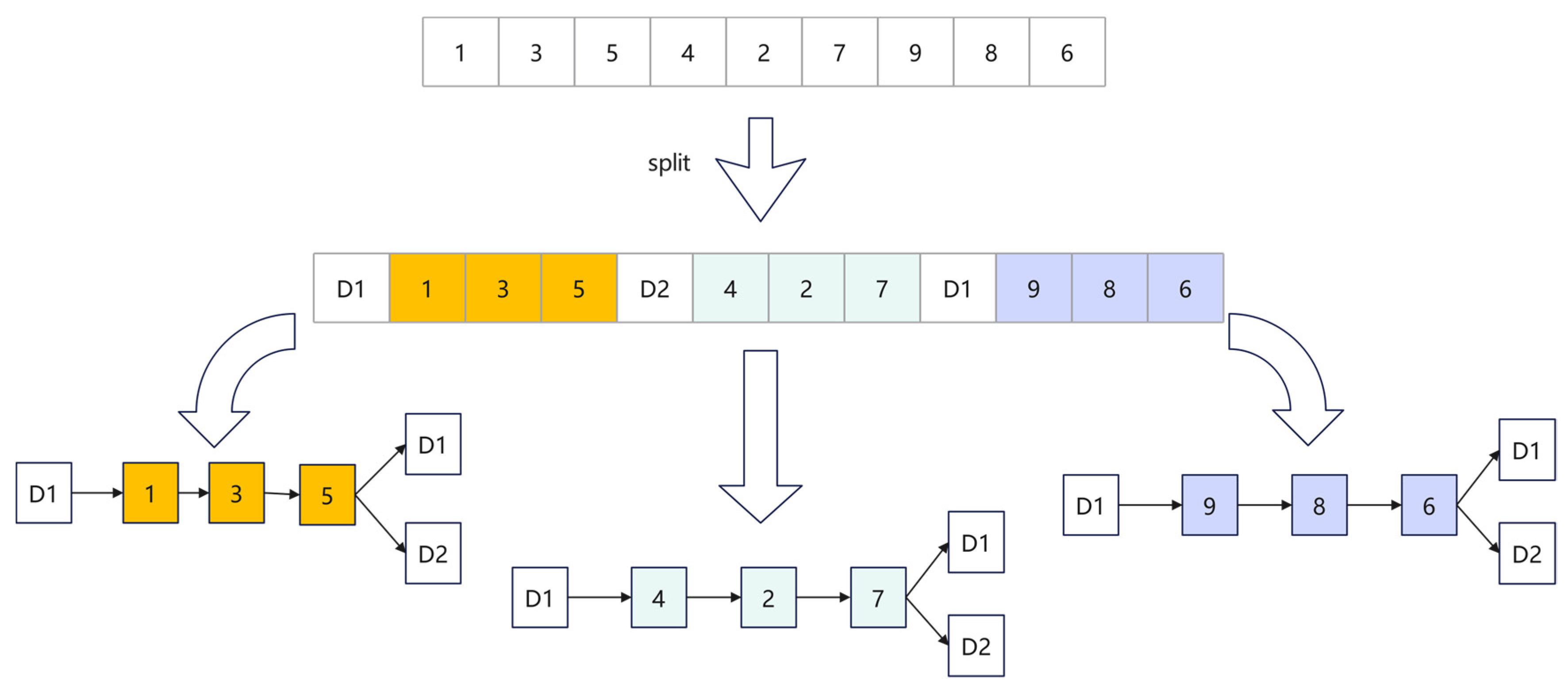
4.1. The Split for the GVRPDS

In the basic Split [11], the label $V_j$ on node $j$ of the auxiliary graph $H$ is the minimum cost of connecting the path from virtual node 0 to node $j$. For GVRPDS, we have to choose a yard for each arc in $H$, so that the resource consumption of $r_1,r_2,\dots ,$ the $r_n$ of each path (the number of vehicles used by each parking lot) does not exceed $p_1,p_2,\dots ,p_n$ (number of parking spaces per car park). In this case, finding the lowest carbon emission path becomes a resource-constrained shortest path problem (RCSPP). In this paper, by using the multi-label extension of the Bellman algorithm [43], the RCSPP of GVRPDS can be solved quickly enough in practice. Each node is labeled (Q|$r_1,r_2,\dots$), Q is the total carbon emission of the node, $r_1,r_2,\dots$ is the vehicle to be used when selecting different depots. In practice, for each node, different carbon emissions will be generated for each vehicle location and a different number of vehicles will be used, which will generate many labels; at this time, these labels can be removed using the dominance rule, and only the good labels can be retained.

Figure 2 above depicts a small example with three customers (a, b, c) and two depots (D1, D2). The top left circle in Figure 2 represents two alternative depots, D1 and D2, and the numerical value in parentheses next to each depot represents the carbon emissions generated from that depot to the customer point. For example, the carbon emission from D1 to customer a is 5, and the carbon emission from D2 to customer a is 6. The requirements of a, b, and c are 5, 4, and 4, respectively. The given order T = (a, b, c) materialized on the left as a giant trip to show the carbon emissions generated between customers and between customers and various car yards, assuming vehicle capacity Q = 10. A list of labels is generated by each node, as shown in the lower part of the figure. Because the dominance rule reserves only one label, the label of the final node c is (21|1, 1). Therefore, the three customers of abc are optimally divided into ab assigned to D1 depot and c assigned to D2 depot as shown in the upper right part of the figure.

4.2. Encoding and Decoding

Considering the coexistence of multiple parking yards and customers’ time requirements, it is difficult to solve. In this paper, an indirect coding method is constructed, that is, the sequence contains no parking yard information and only consists of customer nodes, and the constraints such as capacity, time, and mileage are handed over to the Split for processing. In this way, there is no need to check or repair infeasible solutions repeatedly in algorithm iteration, which facilitates the search process of the algorithm.

The process of decoding is illustrated in Figure 3. In this example, nine customers and two depots are considered. First, a random sequence of customers is divided into the optimal path using the Split algorithm. Once the vehicle reaches the last customer on the designated route, it assesses the distance to each depot and the available parking spaces at each location, then selects the most suitable depot for its return.

4.3. The Initial Solution

The initial solution is generated based on the Split Insertion method, which mainly contains three steps.

Step 1: Build a secondary graph with all customer nodes and virtual starting points to initialize labels for each node, including the minimum cost of the connection path. Each node’s label will be used to store the carbon emission of the path from the virtual starting point to that node and other relevant information.

Step 2: Randomly select a customer as the starting customer and set it as the first customer on the current path. The customer’s label will be updated to reflect the carbon emissions of connecting from the virtual node to the customer. Consider the other customers in turn from the current customer, and calculate the insertion carbon emission for each customer at each insertion location in the current path. Insert the customer into the current path by traversing the insertion locations and selecting the lowest carbon emission insertion point. Update the path’s label information to ensure that newly inserted customers do not affect the path’s constraints, and if the current path does not meet all constraints, end the path and re-select other customers to build the new path.

Step 3: Repeat the above steps until all customers have been successfully inserted into the appropriate path. Each time a new customer is inserted, the carbon emission of the path is reassessed and the label information is updated. Finally, an initial feasible solution satisfying all constraints is generated.

4.4. Search Mechanism

On the basis of generating the initial feasible solution, the current solution sequence is reconstructed by applying removal and insertion operators in ALNS to expand the neighborhood and improve the search space. For instance, consider a problem with six customers, where the initial solution consists of two paths, as depicted in Figure 4A. The removal and insertion operators are selected based on the roulette wheel mechanism. In Figure 4B, the removal operator eliminates customer 2, resulting in a corrupted solution and a removal set. Then, the insertion operator reintroduces customer 2, creating a new neighborhood solution, as shown in Figure 4C. When reinserting a customer, it is essential to update the time variables for each route in the model, as the objective value of the new solution could change considerably.

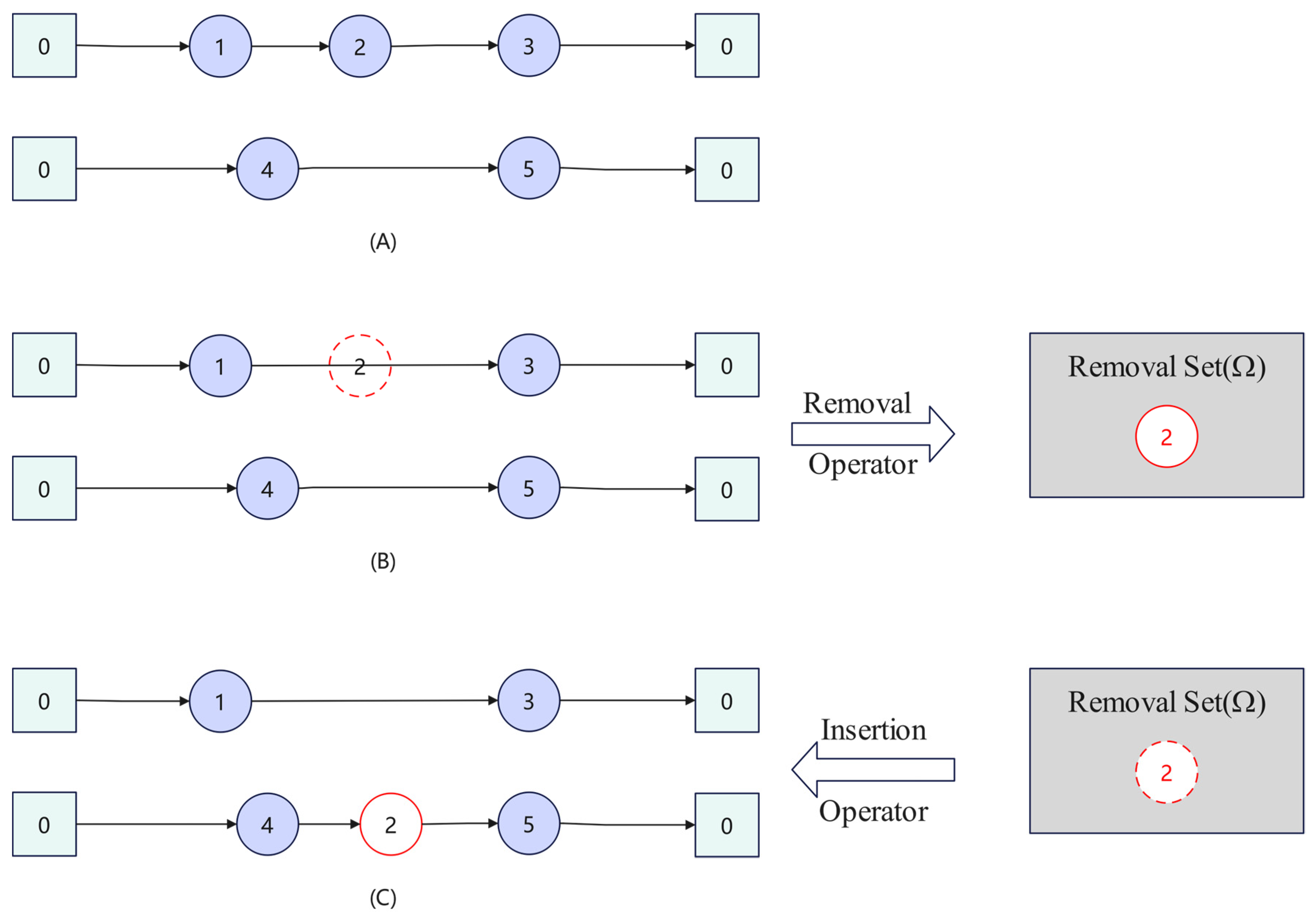
4.4.1. Removal Operators

The removal operator aims to enhance search diversity by eliminating specific customers from the solution while maintaining its overall structure. The probability of selecting each destructive heuristic is dynamically updated based on its performance over iterations. Five removal operators are employed to remove customers from the current solution $S$, with a total of n customers removed from each route $L$ in $S$ and added to the removal list $\Gamma$ during the process.

Existing removal operators Three removal operators currently in use are summarized briefly as follows:

1. Random removal: This operator refers to randomly selecting a certain percentage of customers in the solution.

2. Worst removal: The purpose of this operator is to remove the p customers that contribute the most significant change in total carbon emission.

3. Worst route removal: The goal of the worst route removal operator is to eliminate the entire route with the highest carbon emission.

Innovative removal operators The relocation operators mentioned earlier do not consider the quality of the selected customers, as they are chosen randomly. However, given the specific nature of the problem at hand, we assess whether a chosen customer can be effectively integrated into a route by evaluating the potential cost savings. Based on this evaluation, we have developed two new removal operations that focus on minimizing carbon emissions to the greatest extent possible.

1. Carbon emission-optimization removal: This operator identifies customers that can be removed from a route and inserted in a position that results in a lower carbon emission. $v$ represents the removed customer, $i_1$ and $j_1$ denote the front and back nodes of $v$, and $\left(i_1,j_1\right)$ represents the arc where $v$ can be inserted. Therefore, a carbon emission-optimization evaluation criterion is proposed:

$$C_{i_{1}v}+C_{v{j}_1}+C_{i_2{j}_2}>C_{i_1{j}_1}+C_{i_{2}v}+C_{v{j}_2}$$

(13)

$C_{ij}$ represents the carbon emission incurred from $i$ to $j$. The specific procedure for this operator is outlined in Algorithm 1.

Algorithm 1	Carbon emission-optimization removal
Input:	$\mathrm{A} \mathrm{feasible} \mathrm{solution} S$, $\mathrm{removal} \mathrm{list} \Gamma$, $\mathrm{total} \mathrm{number} \mathrm{of} \mathrm{iterations} I$
Output:	$\mathrm{Solution}$, $\mathrm{removal} \mathrm{list} \Gamma$;
1.	$\mathrm{Current} \mathrm{iteration} \mathrm{count} \leftarrow$ 0;
2.	while$(\mathrm{Current} \mathrm{iteration} \mathrm{count}<I$) do
3.	$\mathrm{Current} \mathrm{iteration} \mathrm{count} \leftarrow$ Current iteration count + 1;
4.	$\mathrm{Random} \mathrm{select} \mathrm{a} \mathrm{route} L$$\mathrm{from}S$;
5.	$\mathbf{foreach} (\mathrm{customer} v$$\mathrm{in} L$) do
6.	$\mathrm{Let} \mathrm{node} i_1$, $j_1$$\mathrm{denote} \mathrm{the} \mathrm{previous} \mathrm{and} \mathrm{next} \mathrm{nodes} \mathrm{of} v$ $\mathrm{in} L$;
7.	foreach$(\mathrm{route} L$$\mathrm{in} S$) do
8.	foreach$(\mathrm{arc} \left(i_2,j_2\right)$$\mathrm{in} L$) do
9.	if$(\mathrm{customer} v$$\mathrm{can} \mathrm{be} \mathrm{inserted} \mathrm{between} \mathrm{the} \mathrm{arc} \left(i_2,j_2\right)$) then
10.	if$(C_{i_{1}v}+C_{v{j}_1}+C_{i_2{j}_2}>C_{i_1{j}_1}+C_{i_{2}v}+C_{v{j}_2}$) then
11.	$\mathrm{Remove} \mathrm{customer} v$$\mathrm{from} L$$, \Gamma \leftarrow \Gamma \cup \left\{v\right\}$;
12.	Return to step 2;

2. Exchange-optimization removal: The exchange-optimization removal operator selects pairs of customers, enabling the simultaneous replacement of one customer with another. Suppose $v_1$ and $v_2$ represent two customers in pairs. The nodes in front of $v_1$ and $v_2$ are $i_1$ and $i_2$, and the nodes in the back are $j_1$ and $j_2$. This removal must satisfy the following condition:

$$C_{i_1{v}_1}+C_{v_1{j}_1}+C_{i_2{v}_2}+C_{v_2{j}_2}>C_{i_1{v}_2}+C_{v_2{j}_1}+C_{i_2{v}_1}+C_{v_1{j}_2}$$

(14)

4.4.2. Repair Operators

The main function of the repair operator is to repair the corrupted solution and generate a new feasible solution based on the Split. These operators are responsible for rationally redistributing the demand nodes removed during the destruction process to the paths in order to satisfy the constraints of the problem and ensure the connectivity of the path while minimizing the total carbon emission. There are three repair operators that will be used, namely, random repair operator, greedy repair operator, and regret repair operator.

1. Random repair operator: The random repair operator is implemented by selecting a customer from the request library and randomly inserting it into the path until all customers in the request library have been inserted.

2. Greedy repair operator: The greedy repair operator tries to insert demand nodes into each possible position of the assigned node sequence one by one based on the removed demand nodes and the assigned node sequence, and calculates the incremental size of the objective function after insertion.

$$F_i=\arg {\min }_{p\in P,i\in IP}f(S_p,i)$$

(15)

Here, $P$ is the set of unassigned demand nodes, $IP$ is the set of possible insertion locations, and $f(S_p,i)$ is the objective function value when the demand node $P$ is inserted into the ith position in $S$.

3. Regret repair operator: The regret repair operator minimizes the total carbon emission of the overall solution by prioritizing the insertion of those nodes that are likely to increase the most carbon emission in the future. The operator first separates the unallocated demand nodes from the allocated demand nodes, and then calculates for each unallocated demand node the difference between the objective function value of the optimal location and the objective function value of the optimal location when inserting at n suboptimal locations, and selects the demand node with the largest sum of differences and its optimal location.

$$D=\arg {\max }_{p\in P}\left\{{\displaystyle {\sum }_{i=2}^n\left(f(s_i(p))-f(s_1(p))\right)}\right\}$$

(16)

Here, $P$ is the set of unassigned demand nodes, and $f(s_i(p))-f(s_1(p))$ is the objective function difference when the demand node $P$ is inserted into the optimal position and the ith suboptimal position in $S$.

4.5. Adaptive Weighting Mechanism

There are two strategies for updating operator weights. One is to update the weights once every time destruction and repair are executed, and the other is to update the weights once every $Pu$ times destruction and repair are executed. The former can ensure that the weight is updated in time, but it needs more calculation time; the latter, by reasonably setting $Pu$ parameter, $Pu$ parameter refers to a parameter used to control the weight update frequency in the ALNS algorithm. Specifically, it affects when to update operator weights, saving computing time, while not being too late to update weights. This paper adopts the latter update strategy.

$$w{(h)}_{j+1}=\left\{\begin{array}{cc}(1-\rho )w{(h)}_j+\rho {\displaystyle \frac{s(h)}{u(h)}},& u(h)>0\\ (1-\rho )w{(h)}_j,& u(h)=0\end{array}\right.$$

(17)

$w{(h)}_j$ represents the operator weight in segment $j$, $\rho$ is the attenuation coefficient, $s(h)$ is the total reward score of the operator, and $u(h)$ is the number of times the operator is selected. The initial value of $s(h)$ is set to zero, the rules of adding points for operators are listed as follows:

(1)

If $y_{new}<y_{best}$, the corresponding operators get ${\delta }_1$ points.

(2)

If $y_{new}\le y_{cur}$ the corresponding operators get ${\delta }_2$ points.

(3)

If $y_{new}>y_{cur}$, but $y_{new}$ is still accepted as $y_{cur}$, the corresponding operators get ${\delta }_3$ points.

For the third case mentioned above, it is proposed for the diversity of solutions searched by the algorithm. Although the solutions searched are worse than the existing solutions, they will be accepted by the acceptance criterion. $\rho$ is the decay coefficient, which controls the influence of the most recently successfully applied operator on its weight. When $\rho =0$, the weight of the operator always remains unchanged. When $\rho =1$, the weight of the previous iteration cycle is independent of the update of the current weight, which is only related to the successful operation of the operator in the current iteration cycle. In order to better highlight the characteristics of adaptive learning, the general setting $0<\rho <1$.

4.6. Acceptance and Stopping Criteria

To prevent the algorithm from getting trapped in a local optimum, we accept not only better solutions but occasionally worse solutions as well. To achieve this, we adopt the acceptance criterion from simulated annealing: the probability $P=e^{-\left[f\left(s^t\right)-f\left(s\right)\right]/T}$ that the new solution is accepted, where $f\left(s^t\right)$ represents the objective function value of the new solution $s^t$ and $f\left(s\right)$ represents the objective function value of the current solution $S$; $T$ is the current temperature value of the simulated annealing algorithm. The initial value of $T$ is set as $\omega f\left(s_0\right)$, the algorithm iterates continuously, and the temperature $T$ is multiplied by a constant annealing rate $phi,$ $phi\in$(0,1) with iterations, then the temperature is gradually decreased with $T=phi\ast T$. As the algorithm iterates later, the possibility of accepting inferior solutions is gradually reduced, and almost no inferior solutions are accepted at last, which ensures the convergence of the solution. The algorithm terminates when the number of iterations is reached.

5. Experiments and Analyses

5.1. Instances Generation

In the experiment, no benchmark instance set is available since the GVRPDS model is a new variant of the multi-depot green vehicle routing problem with time windows. But the main difference is that for starting the vehicle and parking space constraints, similar to that of other basic data, Cordeau (2001) and others benchmark examples. There are 18 examples, among which the customer time window from pr01 to pr09 is narrow, and the number of vehicles used for service in the yard is large. The customer time window from pr11 to pr19 is wider, and the number of vehicles used for service in the depot is less. These examples can be divided into the following three types according to the number of customers: small scale cases with 1–100 customers (pro01, pro02, pro07, pro11, pro12, and pro17), medium scale cases with 101–200 customers (pro03, pro04, pro08, pro13, pro14, and pro18) and customers with 201–300 large-scale cases (pro05, pro06, pro09, pro15, pro16, and pro19). Based on this example, the number of parking spaces $P_d$ and the starting available vehicles $K_d$ of the parking lot are added. The following

Table 2. Example data information.

Instances	Number	${\mathit{P}}_{\mathit{d}}$	${\mathit{K}}_{\mathit{d}}$	Depot	Vehicle	Capacity
pro01	48	4	3	4	8	200
pro02	96	6	4	4	12	195
pro03	144	8	6	4	16	150
pro04	192	10	8	4	20	185
pro05	240	12	10	4	24	180
pro06	288	14	12	4	28	175
pro07	72	5	4	6	12	200
pro08	144	8	6	6	18	190
pro09	216	11	10	6	24	180
pro11	48	4	3	4	8	200
pro12	96	6	4	4	12	195
pro13	144	8	6	4	16	150
pro14	192	10	8	4	20	185
pro15	240	12	10	4	24	180
pro16	288	14	12	4	28	175
pro17	72	5	4	6	12	200
pro18	144	8	6	6	18	190
pro19	216	11	10	6	24	180

describes the number of customers, the number of depots, the number of vehicles per depot, the maximum capacity of the vehicles as well as the number of parking spaces and the starting number of available vehicles for the example. All tests were performed on an Intel Core (TM) i7-1200p processor at 2.10 ghz with 16.00 GB of RAM for Windows 11. The introduction of the case can be obtained from the website http://www.iescm.com/vrp/instances.asp, accessed on 15 October 2024.

5.2. Parameter Setting

The parameter setting of ALNS proposed by Ropke and Pisinger [33] is adopted, in which the reward scores of operator ${\delta }_1$, ${\delta }_2$ and ${\delta }_3$ are set as ${\delta }_1$ = 30, ${\delta }_2$ = 20 and ${\delta }_3$ = 10 in this paper. Other relevant parameter settings are shown in the following

Table 3. The parameters of the SALNS algorithms.

Notation	Description	Value
$worst\_d$	Worst-case number of corrupts	[5, 10]
$regret\_n$	Regret value the number of corruptions	5
$rho$	Weight decay ratio	0.1
$phi$	Rate of annealing	0.9
$pu$	Weight adjustment step size	5

.

5.3. SALNS Performance Evaluation

5.3.1. Comparisons SALNS with ALNS

This section aims to verify the performance improvement of the SALNS compared with the classical ALNS [44] through experiments. Each experiment is run 10 times in the experiment, and the best value of the 10 experiments is recorded. Time indicates the CPU time (unit: minutes). To evaluate the difference in solution quality between the SALNS and classical ALNS algorithms, the following formula is used:

$$Ga{p}_1{\displaystyle \frac{O{V}_{classicalALNS}-{OV}_{SALNS}}{{OV}_{classicalALNS}}}\ast 100\%$$

(18)

OV means the objective value.

Table 4. Comparisons SALNS with ALNS on instances.

Instances	SALNS		ALNS		$\mathit{G}\mathit{a}{\mathit{p}}_1$
	Carbon Emission	Time	Carbon Emission	Time
pro01	78.5	1.1	78.5	1.3	0.00%
pro02	169.4	5.7	182.6	6.7	7.23%
pro03	272.3	15.9	300.5	16.4	9.38%
pro04	404.5	24.2	465.6	28.5	13.12%
pro05	416.0	43.4	470.2	48.0	11.49%
pro06	512.3	62.3	603.7	65.6	15.14%
pro07	137.3	4.9	137.3	5.2	0.00%
pro08	271.5	17.0	292.3	21.6	7.12%
pro09	375.2	27.8	400.9	30.3	6.41%
pro11	74.5	0.8	74.5	1.0	0.00%
pro12	126.4	5.9	144.3	6.0	12.40%
pro13	210.7	14.4	230.7	15.2	8.67%
pro14	214.5	25.5	243.6	29.7	11.95%
pro15	302.6	46.3	321.8	52.3	5.97%
pro16	358.6	65.4	415.4	75.4	13.67%
pro17	103.5	4.3	115.9	4.7	10.70%
pro18	216.3	16.0	242.7	17.1	10.88%
pro19	275.4	66.7	302.3	70.5	8.90%

presents the comparison between SALNS and the classic ALNS in terms of total carbon emission across different instances. The results indicate that SALNS outperforms ALNS in most instances. In the pro02 instance, SALNS achieves a 7.23% reduction in carbon emissions compared to ALNS, while also reducing the computation time by 14.93%. Similarly, in pro04, SALNS results in a 13.12% reduction in carbon emissions and also shows a faster runtime by 15.08%. The best improvement in carbon emissions is observed in the pro06 instance, with a reduction of 15.14%. There are instances like pro01, pro07, and pro11 where both SALNS and ALNS yield identical results for carbon emissions (0.00% improvement), suggesting that the algorithms perform similarly in small instances. The speed of finding solutions in all instances in SALNS is better than ALNS, as evidenced by the generally shorter computation times. This demonstrates that SALNS provides a significant improvement over ALNS, both in terms of carbon emissions reduction and computational efficiency.

To assess the performance of the innovative removal operators, we use instances (pr01–pr09) to demonstrate their superiority. The ALNS, which incorporates only the three current removal operators, is presented in the table labeled “General”. The ALNS with General and Carbon emission optimization removal is represented in the table under the “COR” heading. The ALNS with General and Exchange optimization Removal is represented in the table under the “EOR” heading.

Table 5. Comparison of the results of different removal operators for ALNS.

Instances	General		COR		EOR
	Carbon Emission	Time	Carbon Emission	Time	Carbon Emission	Time
pro01	78.5	1.3	78.5	1.1	78.5	1.2
pro02	176.7	6.2	172.6	6.3	173.4	6.2
pro03	294.3	16.4	284.5	16.2	287.3	16.3
pro04	409.5	28.5	405.6	25.5	407.6	26.5
pro05	430.2	48.0	420.2	47.0	421.2	46.1
pro06	528.5	65.6	523.7	65.3	518.7	64.6
pro07	137.3	5.2	137.3	5.0	137.3	5.0
pro08	290.3	21.6	284.3	20.6	286.6	19.6
pro09	402.9	30.3	394.9	28.3	395.3	29.3

compares these three categories of ALNS algorithms and two removal operators (COR and EOR) improve the average accuracy by 1.55%, and 1.32%. This shows the good performance of the innovative removal operators.

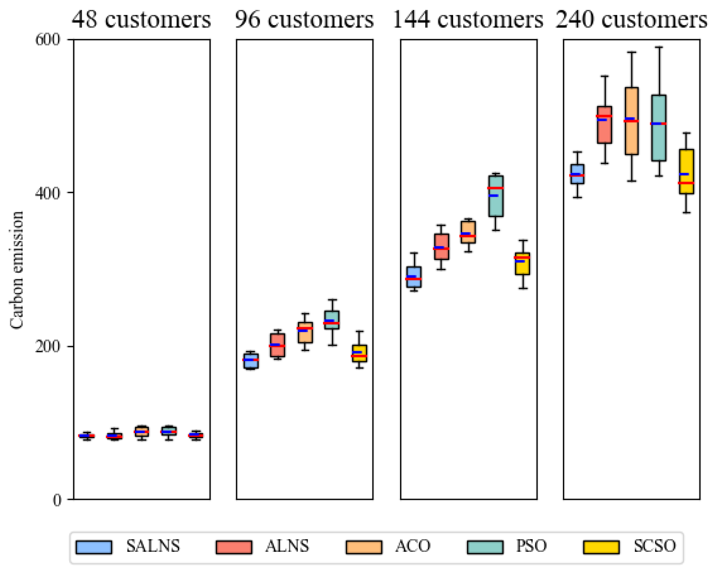
5.3.2. Comparisons with Meta-Heuristic Algorithms

In order to further assess the effectiveness of the SALNS, the test results of SALNS are compared with several representative algorithms (ant colony algorithm (ACO) [45], particle swarm optimization algorithm (PSO) [46] and sand cat swarm optimization algorithm (SCSO) [47]) used to solve the MDVRP problem.

To ensure a fair comparison and strengthen the reliability of the analysis, the parameters for ACO, PSO, and SCSO algorithms were carefully set based on their respective foundational literature and recent studies. For ACO, the parameters include a pheromone importance factor α of 2.0, a heuristic importance factor β of 2.0, a pheromone evaporation rate ρ of 0.8, and an ant population size m of 30. For PSO, the settings include a swarm size n of 30, an inertia weight ω of 0.7, cognitive and social learning factors $c_1$ of 1.5 and $c_2$ of 4, and a velocity range of [−2, 2]. For SCSO, the parameters involve a population size n of 30, a sensitivity range $r_G$ of [0, 2], and a phase control range R of $[-2r_G,2r_G]$. The number of iterations is 500. These settings ensure the use of the best-performing versions of the algorithms and align with their application in solving the GVRPDS, as confirmed by experimental validation.

The experimental results in

Table 6. Comparisons SALNS with meta-heuristic algorithms on instances.

Instances	SALNS		ACO		PSO		SCSO
	Carbon Emission	Time	Carbon Emission	Time	Carbon Emission	Time	Carbon Emission	Time
pro01	78.5	1.1	78.5	1.3	78.5	1.2	78.5	1.1
pro02	169.4	5.7	194.2	6.6	201.2	7.2	172.3	5.8
pro03	272.3	15.9	323.5	18.7	350.3	17.0	275.4	19.3
pro04	404.5	24.2	433.1	27.0	436.2	31.2	402.1	34.7
pro05	416.0	43.4	446.2	50.2	452.6	48.1	412.3	45.6
pro06	512.3	62.3	570.8	65.4	563.6	63.2	524.2	65.2
pro07	137.3	4.9	145.1	5.1	227.3	5.4	134.2	5.6
pro08	271.5	17.0	323.6	24.3	342.5	23.1	300.4	18.4
pro09	375.2	27.8	412.2	33.4	420.5	30.3	430.2	35.6
pro11	74.5	0.8	74.5	1.1	74.5	0.9	74.5	0.7
pro12	126.4	5.9	137.4	6.4	144.3	7.9	127.4	5.6
pro13	210.7	14.4	218.3	15.8	224.3	16.8	208.4	17.3
pro14	214.5	25.5	232.2	26.9	253.6	26.7	223.5	27.4
pro15	302.6	46.3	371.6	50.9	360.6	53.2	345.2	56.3
pro16	358.6	65.4	403.7	70.7	433.9	73.2	385.2	72.8
pro17	103.5	4.3	121.3	5.2	125.6	5.1	105.3	4.4
pro18	216.3	16.0	256.5	19.2	260.3	18.8	224.9	16.6
pro19	275.4	66.7	301.6	70.3	315.6	73.4	295.4	75.3

show that the SALNS is significantly effective in solving instances compared to the other two kinds of algorithms. The average improvement rates of SALNS over PSO, ACO, and SCSO on instances are 9.48%, 13.79%, and 3.27%. In addition, as shown in Table 6, in terms of computational efficiency, compared with other algorithms, the calculation time of SALNS is significantly shorter, and the solution obtained in shorter time is also better than other algorithms, which reflects the excellent search efficiency and excellent performance of SALNS. From the experimental results, although SALNS shows strong performance in most instances, there are special cases, which need further analysis. In instances such as pro01 and pro11, the performance of the algorithms tends to be consistent, possibly reflecting the simplicity of these instances and the smaller optimization space of the algorithms. For these instances, complex optimization strategies may not be necessary and the differences between different algorithms are small.

To assess the robustness of the SALNS, we utilized box plots to display the median, variability, and outliers from several iterations. These plots illustrate the performance of the SALNS, ALNS, ACO, PSO, and SCSO algorithms for each instance. Take pro01 (48 customers), pro02 (96 customers), pro03 (144 customers), and pro05 (240 customers) as an example.

In Figure 5, the red line represents the median and the blue line represents the mean. The experimental results showed that SALNS demonstrated the lowest median carbon footprint and smaller quartile spread when dealing with a problem size of 48 to 240 customers, demonstrating not only its effectiveness in reducing carbon emissions, but also the high stability of its results. As the number of customers increased, although the carbon emissions of all algorithms rose, SALNS showed relatively small increases and were less sensitive to outliers, showing strong robustness.

5.4. Evaluation of Question Features

The strategy of the depot sharing is proposed to reduce the additional distance of the vehicle returning to the depot after serving the last customer, so as to maximize the reduction of carbon emissions. In order to verify the effectiveness of this strategy, this section will compare the total carbon emission of returning to the original depot and the depot resource sharing, and the optimization rate of the carbon emission, and the results are shown in the Figure 6. To measure the difference in carbon emission between depot sharing and returning to the original depot, the following equation is used:

$$Ga{p}_2={\displaystyle \frac{C_{ROD}-C_{DS}}{C_{ROD}}}$$

(19)

$C_{ROD}$ represents the carbon emission of returning to the original depot, $C_{DS}$ represents the carbon emission of the depot sharing.

As shown in Figure 6, the depot sharing has a certain improvement in the total carbon emission compared to returning to the original depot. The optimization rates of carbon emission for small-scale examples pro01, pro02, pro07, pro11, pro12, and pro17 are 3.4%, 7.0%, 5.5%, 7.3%, 12.0%, and 7.7%. For the medium-scale examples pro03, pro04, pro08, pro13, pro14, and pro18, the optimization rates of carbon emission are 20.1%, 16.8%, 6.8%, 6.5%, 8.5%, and 9.2%. For large-scale examples pro05, pro06, pro09, pro15, pro16, and pro19, the optimization rates of carbon emission are 15.7%, 17.9%, 9.1%, 15.3%, 8.1%, and 5.6%. It can be seen that the strategy of the depot sharing can reduce carbon emissions when solving GVRPDS.

5.5. The Sensitivity Analysis of Model Parameters

To further investigate the proposed model and its practical implications, a sensitivity analysis was conducted. This analysis focuses on evaluating the effects of vehicle speed and driving distance on carbon emissions. A set of sensitivity analysis experiments is designed in this section. Five instances (pro01–pro05) were selected to conduct experiments at three different speeds (30 km/h, 40 km/h, and 50 km/h), and the changes in carbon emissions were compared.

As shown in

Table 7. Carbon emissions under different speeds.

Instances	30 km/h		40 km/h		50 km/h
	Carbon Emission	Distance	Carbon Emission	Distance	Carbon Emission	Distance
pro01	83.4	645.2	78.5	610.4	71.4	594.4
pro02	183.6	1369.3	169.4	1274.3	153.6	1185.0
pro03	300.5	1944.4	272.3	1775.7	258.1	1347.2
pro04	432.1	2597.2	404.5	2383.7	384.6	2234.9
pro05	440.2	2674.1	416.0	2400.5	396.7	2356.5

, the speed increased from 30 km/h to 50 km/h, carbon emissions showed an overall downward trend, and the average reduction of carbon emissions in each case was between 10% and 15%. This suggests that increasing speed significantly reduces fuel consumption at idle and low speeds, thereby reducing carbon emissions. At the same time, when the speed is the same, the influence of driving distance on carbon emission increases linearly, and carbon emission increases correspondingly with the increase in driving distance. In the green vehicle routing problem, rational optimization of route planning can reduce the driving distance and thus reduce carbon emissions.

6. Conclusions

The green vehicle routing problem with depot sharing is presented in this paper. Considering the constraints of vehicle load, driving distance, time window, starting vehicle number of each depot, and parking number of each depot, a model with the objective of minimizing the total carbon emission was established. For the complex vehicle routing problem, an improved adaptive large neighborhood search algorithm is proposed. The Split performs the best route splitting for a given sequence, and ALNS performs the local and global solution search. In addition, two innovative removal operators enhance the diversification capability of ALNS. After the analysis of examples, the proposed solution is proven to be superior to the classical ALNS, PSO, and ACO. Finally, an example is given to prove that the strategy of the depot resource sharing not only increases the flexibility of transportation operation, but also effectively reduces carbon emissions.

The findings of this study have to be seen in light of some limitations. Firstly, all vehicles in the model run at a uniform speed, which is different from the actual situation. In reality, the speed of a vehicle is usually affected by many factors, such as traffic conditions, road slope, and driver operation. Therefore, the variable speed characteristics of the vehicle are not fully considered in the model. Future research can further consider the carbon emissions generated by the variable speed case of the vehicle under different conditions. Secondly, the current model assumes that the fleet is composed of homogeneous vehicles, while in reality, the vehicle types are usually diverse, including traditional fuel vehicles, electric vehicles, and hybrid electric vehicles. The differences in energy efficiency, emission characteristics, charging, and refueling infrastructure of different types of vehicles are not considered.

Therefore, it is possible to consider introducing heterogeneous fleets into the model in the future, including traditional fuel vehicles, electric vehicles, and hybrid electric vehicles, while taking into account the differences in energy consumption, emission characteristics, charging, and refueling infrastructure of different types of vehicles. According to the energy efficiency and emission characteristics of each vehicle, the energy consumption and emission calculation are introduced to optimize the route and reduce energy waste and carbon emissions. In addition, considering the infrastructure requirements of different vehicles, the model can take the availability of charging stations and gas stations as constraints to ensure energy replantation in actual operation. Through these optimizations, the model can not only reduce carbon emissions in green transportation, but also better integrate with the actual logistics system to promote the sustainable development of green logistics.

References

1. Choi, D.; Gao, Z.; Jiang, W. Attention to Global Warming. Rev. Financ. Stud. 2020, 33, 1112–1145. [Google Scholar] [CrossRef]
2. Zhang, W.; Gajpal, Y.; Appadoo, S.S.; Wei, Q. Multi-Depot Green Vehicle Routing Problem to Minimize Carbon Emissions. Sustainability 2020, 12, 3500. [Google Scholar] [CrossRef]
3. Duan, H.; Zhou, S.; Jiang, K.; Bertram, C.; Harmsen, M.; Kriegler, E.; Van Vuuren, D.P.; Wang, S.; Fujimori, S.; Tavoni, M.; et al. Assessing China’s Efforts to Pursue the 1.5 °C Warming Limit. Science 2021, 372, 378–385. [Google Scholar] [CrossRef] [PubMed]
4. Erdoğan, S.; Miller-Hooks, E. A Green Vehicle Routing Problem. Transp. Res. Part E Logist. Transp. Rev. 2012, 48, 100–114. [Google Scholar] [CrossRef]
5. Moghdani, R.; Salimifard, K.; Demir, E.; Benyettou, A. The Green Vehicle Routing Problem: A Systematic Literature Review. J. Clean. Prod. 2021, 279, 123691. [Google Scholar] [CrossRef]
6. Nura, A.; Abdullahi, S. A Systematic Review of Multi-Depot Vehicle Routing Problems. Syst. Lit. Rev. Meta-Anal. J. 2022, 3, 51–60. [Google Scholar] [CrossRef]
7. Eglese, R.; Bektas, T. Chapter 15: Green Vehicle Routing. In Vehicle Routing: Problems, Methods, and Applications, 2nd ed.; Toth, P., Vigo, D., Eds.; MOS-SIAM Series on Optimization; Society for Industrial and Applied Mathematics: Philadelphia, PA, USA, 2014; pp. 437–458. [Google Scholar] [CrossRef]
8. Lahyani, R.; Gouguenheim, A.-L.; Coelho, L.C. A Hybrid Adaptive Large Neighbourhood Search for Multi-Depot Open Vehicle Routing Problems. Int. J. Prod. Res. 2019, 57, 6963–6976. [Google Scholar] [CrossRef]
9. Alinaghian, M.; Shokouhi, N. Multi-Depot Multi-Compartment Vehicle Routing Problem, Solved by a Hybrid Adaptive Large Neighborhood Search. Omega 2018, 76, 85–99. [Google Scholar] [CrossRef]
10. Mühlbauer, F.; Fontaine, P. A Parallelised Large Neighbourhood Search Heuristic for the Asymmetric Two-Echelon Vehicle Routing Problem with Swap Containers for Cargo-Bicycles. Eur. J. Oper. Res. 2021, 289, 742–757. [Google Scholar] [CrossRef]
11. Prins, C.; Lacomme, P.; Prodhon, C. Order-First Split-Second Methods for Vehicle Routing Problems: A Review. Transp. Res. Part C Emerg. Technol. 2014, 40, 179–200. [Google Scholar] [CrossRef]
12. Lin, C.; Choy, K.L.; Ho, G.T.; Chung, S.H.; Lam, H.Y. Survey of Green Vehicle Routing Problem: Past and Future Trends. Expert Syst. Appl. 2014, 41, 1118–1138. [Google Scholar] [CrossRef]
13. Bektaş, T.; Laporte, G. The Pollution-Routing Problem. Transp. Res. Part B Methodol. 2011, 45, 1232–1250. [Google Scholar] [CrossRef]
14. Park, Y.; Chae, J. A Review of the Solution Approaches Used in Recent G-VRP (Green Vehicle Routing Problem). Int. J. Adv. Logist. 2014, 3, 27–37. [Google Scholar] [CrossRef]
15. Rezaei, N.; Ebrahimnejad, S.; Moosavi, A.; Nikfarjam, A. A Green Vehicle Routing Problem with Time Windows Considering the Heterogeneous Fleet of Vehicles: Two Metaheuristic Algorithms. Eur. J. Ind. Eng. 2019, 13, 507–535. [Google Scholar]
16. Schneider, M.; Stenger, A.; Goeke, D. The Electric Vehicle-Routing Problem with Time Windows and Recharging Stations. Transp. Sci. 2014, 48, 500–520. [Google Scholar] [CrossRef]
17. Amiri, A.; Amin, S.H.; Zolfagharinia, H. A Bi-Objective Green Vehicle Routing Problem with a Mixed Fleet of Conventional and Electric Trucks: Considering Charging Power and Density of Stations. Expert Syst. Appl. 2023, 213, 119228. [Google Scholar] [CrossRef]
18. Liu, Y.; Yu, Y.; Zhang, Y.; Baldacci, R.; Tang, J.; Luo, X.; Sun, W. Branch-Cut-and-Price for the Time-Dependent Green Vehicle Routing Problem with Time Windows. INFORMS J. Comput. 2023, 35, 14–30. [Google Scholar] [CrossRef]
19. Ghannadpour, S.F. Evolutionary Approach for Energy Minimizing Vehicle Routing Problem with Time Windows and Customers’ Priority. Int. J. Transp. Eng. 2019, 6, 237–264. [Google Scholar]
20. Lu, F.; Du, Z.; Wang, Z.; Wang, L.; Wang, S. Towards Enhancing the Crowdsourcing Door-to-Door Delivery: An Effective Model in Beijing. JIMO 2025, 21, 2371–2395. [Google Scholar] [CrossRef]
21. Yang, D.; Hyland, M.F.; Jayakrishnan, R. Tackling the Crowdsourced Shared-Trip Delivery Problem at Scale with a Novel Decomposition Heuristic. Transp. Res. Part E Logist. Transp. Rev. 2024, 188, 103633. [Google Scholar] [CrossRef]
22. Cassidy, P.J.; Bennett, H.S. TRAMP—A Multi-Depot Vehicle Scheduling System. J. Oper. Res. Soc. 1972, 23, 151–163. [Google Scholar] [CrossRef]
23. Yu, B.; Yang, Z.-Z.; Xie, J.-X. A Parallel Improved Ant Colony Optimization for Multi-Depot Vehicle Routing Problem. J. Oper. Res. Soc. 2011, 62, 183–188. [Google Scholar] [CrossRef]
24. Özger, A. Multi-Depot Heterogeneous Fleet Vehicle Routing Problem with Time Windows: Airline and Roadway Integrated Routing. Int. J. Ind. Eng. Comput. 2022, 13, 435–456. [Google Scholar]
25. Fan, H.; Yang, X.; Li, D.; Li, Y.; Liu, P.; Wu, J.X. Half-Open Multi-Depot Vehicle Routing Problem Based on Joint Distribution Mode of Fresh Food. Comput. Integ. Manufact. Syst 2019, 25, 256–266. [Google Scholar]
26. Schmidt, C.E.; Silva, A.C.; Darvish, M.; Coelho, L.C. Time-Dependent Fleet Size and Mix Multi-Depot Vehicle Routing Problem. Int. J. Prod. Econ. 2023, 255, 108653. [Google Scholar] [CrossRef]
27. Soriano, A.; Gansterer, M.; Hartl, R.F. The Multi-Depot Vehicle Routing Problem with Profit Fairness. Int. J. Prod. Econ. 2023, 255, 108669. [Google Scholar] [CrossRef]
28. Salehi Sarbijan, M.; Behnamian, J. Feeder Vehicle Routing Problem in a Collaborative Environment Using Hybrid Particle Swarm Optimization and Adaptive Learning Strategy. Environ. Dev. Sustain. 2023, 1–41. [Google Scholar] [CrossRef]
29. Jabir, E.; Panicker, V.V.; Sridharan, R. Design and Development of a Hybrid Ant Colony-Variable Neighbourhood Search Algorithm for a Multi-Depot Green Vehicle Routing Problem. Transp. Res. Part D Transp. Environ. 2017, 57, 422–457. [Google Scholar] [CrossRef]
30. Shen, L.; Tao, F.; Wang, S. Multi-Depot Open Vehicle Routing Problem with Time Windows Based on Carbon Trading. Int. J. Environ. Res. Public Health 2018, 15, 2025. [Google Scholar] [CrossRef]
31. Qin, G.; Tao, F.; Li, L. A Vehicle Routing Optimization Problem for Cold Chain Logistics Considering Customer Satisfaction and Carbon Emissions. Int. J. Environ. Res. Public Health 2019, 16, 576. [Google Scholar] [CrossRef]
32. Wen, M.; Sun, W.; Yu, Y.; Tang, J.; Ikou, K. An Adaptive Large Neighborhood Search for the Larger-Scale Multi Depot Green Vehicle Routing Problem with Time Windows. J. Clean. Prod. 2022, 374, 133916. [Google Scholar] [CrossRef]
33. Ropke, S.; Pisinger, D. An Adaptive Large Neighborhood Search Heuristic for the Pickup and Delivery Problem with Time Windows. Transp. Sci. 2006, 40, 455–472. [Google Scholar] [CrossRef]
34. Chen, S.; Chen, R.; Wang, G.-G.; Gao, J.; Sangaiah, A.K. An Adaptive Large Neighborhood Search Heuristic for Dynamic Vehicle Routing Problems. Comput. Electr. Eng. 2018, 67, 596–607. [Google Scholar] [CrossRef]
35. Liu, R.; Tao, Y.; Xie, X. An Adaptive Large Neighborhood Search Heuristic for the Vehicle Routing Problem with Time Windows and Synchronized Visits. Comput. Oper. Res. 2019, 101, 250–262. [Google Scholar] [CrossRef]
36. Azi, N.; Gendreau, M.; Potvin, J.-Y. An Adaptive Large Neighborhood Search for a Vehicle Routing Problem with Multiple Routes. Comput. Oper. Res. 2014, 41, 167–173. [Google Scholar] [CrossRef]
37. Gu, W.; Cattaruzza, D.; Ogier, M.; Semet, F. Adaptive Large Neighborhood Search for the Commodity Constrained Split Delivery VRP. Comput. Oper. Res. 2019, 112, 104761. [Google Scholar] [CrossRef]
38. Sacramento, D.; Pisinger, D.; Ropke, S. An Adaptive Large Neighborhood Search Metaheuristic for the Vehicle Routing Problem with Drones. Transp. Res. Part C Emerg. Technol. 2019, 102, 289–315. [Google Scholar] [CrossRef]
39. Koç, Ç.; Bektaş, T.; Jabali, O.; Laporte, G. The Impact of Depot Location, Fleet Composition and Routing on Emissions in City Logistics. Transp. Res. Part B Methodol. 2016, 84, 81–102. [Google Scholar] [CrossRef]
40. Scora, G.; Barth, M. Comprehensive Modal Emissions Model (Cmem), Version 3.01. User Guide; Centre for Environmental Research and Technology, University of California,: Riverside, CA, USA, 2006; Volume 1070, p. 1580. [Google Scholar]
41. Demir, E.; Bektaş, T.; Laporte, G. An Adaptive Large Neighborhood Search Heuristic for the Pollution-Routing Problem. Eur. J. Oper. Res. 2012, 223, 346–359. [Google Scholar] [CrossRef]
42. Niu, Y.; Yang, Z.; Chen, P.; Xiao, J. Optimizing the Green Open Vehicle Routing Problem with Time Windows by Minimizing Comprehensive Routing Cost. J. Clean. Prod. 2018, 171, 962–971. [Google Scholar] [CrossRef]
43. Desrochers, M. An algorithm for the shortest path problem with resource constraints. In Proceedings of the IEEE Conference on Computer Vision and Pattern Recognition (CVPR), Ann Arbor, MI, USA, 5–9 June 1988; pp. 3454–3461. [Google Scholar]
44. Mancini, S. A Real-Life Multi Depot Multi Period Vehicle Routing Problem with a Heterogeneous Fleet: Formulation and Adaptive Large Neighborhood Search Based Matheuristic. Transp. Res. Part C Emerg. Technol. 2016, 70, 100–112. [Google Scholar] [CrossRef]
45. Ky Phuc, P.N.; Phuong Thao, N.L. Ant Colony Optimization for Multiple Pickup and Multiple Delivery Vehicle Routing Problem with Time Window and Heterogeneous Fleets. Logistics 2021, 5, 28. [Google Scholar] [CrossRef]
46. Ramadhani, B.N.I.F.; Garside, A.K. Particle Swarm Optimization Algorithm to Solve Vehicle Routing Problem with Fuel Consumption Minimization. J. Optimasi Sist. Ind. 2021, 20, 1–10. [Google Scholar] [CrossRef]
47. Seyyedabbasi, A.; Kiani, F. Sand Cat Swarm Optimization: A Nature-Inspired Algorithm to Solve Global Optimization Problems. Eng. Comput. 2023, 39, 2627–2651. [Google Scholar] [CrossRef]
Figure 1. The flowchart of SALNS designed for GVRPDS.
Mathematics 13 00214 g001
Figure 2. Example of the Split.
Mathematics 13 00214 g002
Figure 3. The process of decoding.
Mathematics 13 00214 g003
Figure 4. An example for GVRPDS.
Mathematics 13 00214 g004
Figure 5. Boxplots of the carbon emission for five algorithms at different scale instances.
Mathematics 13 00214 g005
Figure 6. Return to the comparison between the original depot and the depot sharing.
Mathematics 13 00214 g006