Digital Twin-Empowered Robotic Arm Control: An Integrated PPO and Fuzzy PID Approach

Abstract

With rapid advancements in digital twin technology within the Industrial Internet of Things, integrating digital twins with industrial robotic arms presents a promising direction. This integration promotes the remote operation and intelligence of industrial control processes. However, the control and error management of robotic arms in digital twin systems pose challenges. In this paper, we present a digital twin-empowered robotic arm system and propose a control policy using deep reinforcement learning, specifically the proximal policy optimization approach. The construction and functionality of each subsystem within the digital twin-empowered robotic arm control system are detailed. To address errors caused by mechanical structure and virtual–real mapping in the digital twin, an integrated proximal policy optimization and fuzzy PID approach is proposed. Experimental results demonstrate that proximal policy optimization is adaptable to virtual–real mapping errors, while the fuzzy PID method corrects physical errors quickly and accurately. The robotic arm can reach the target point using this integrated approach. Overall, error management problems in digital systems have been well addressed, and our scheme can provide an accurate and adaptive control strategy for the robotic arm.

1. Introduction

Robotic arms have become widely used in various industrial production aspects [1]. They are highly flexible and precise, making them significant tools for improving production efficiency and quality [2]. The robotic arms consist of multiple joints and end-loading actuators. The position and posture of the robotic arm can be altered by controlling the joint motor to carry out different tasks. However, the task and trajectory planning of robotic arms has always been a significant challenge worth exploring. Currently, teaching and manual command control are mainstream planning methods used for robotic arms [3]. Nonetheless, these approaches are time-consuming and fail to adapt to changing tasks. If the working environment of the manipulator is changed, it will take a long time to design and debug the program, which greatly affects the efficiency. Therefore, the manufacturing industry has put forward higher requirements for the performance of industrial robotic arms, hoping that these arms can automate decision-making in changing work environments. It is also necessary to equip the robotic arms with a more digital platform for management and maintenance.

Digital twin (DT) technology involves real-time mapping of a physical entity or system in a virtual space. There have been extensive discussions on the deployment of the DT system and the optimization of resource allocation to ensure that the DT system can achieve real-time communication, which provides a basis for practical applications [4].

Real-time monitoring, fault analysis, and full life cycle maintenance of objects constructed in virtual space can be achieved through the utilization of sensors, low-latency Industrial Internet of Things (IIoT), and system modeling technologies [5,6,7,8]. The cloud-based digital twin (CDT) system is a DT system that deploys the parameters of an object in the cloud computing center, which is suitable for the IIoT framework. Within the CDT framework, communication, control, and computing capabilities can be integrated, enabling the utilization of cloud computing resources for additional tasks such as remote collaboration, data mining, machine learning, or the deployment of reinforcement learning (RL) algorithms for control policies [9,10]. Therefore, industrial devices, such as DT objects, can rely on the CDT framework to expand computing tasks. Obviously, industrial robotic arms can also utilize the CDT framework to facilitate remote operation, while allowing for the deployment of additional computing or control tasks to enhance decision-making and automation [11]. The development of DT has broadened the application of artificial intelligence algorithms in robotic arm control.

For instance, RL, as an online optimization method, is suitable for robotic arm control. RL is a subfield of machine learning that focuses on utilizing historical data to improve the future control of dynamic systems [12,13]. Deep reinforcement learning (DRL), in combination with deep neural networks, has demonstrated remarkable performance in addressing high-dimensional and complex control problems, making it an effective solution for the intricate control challenges encountered by robotic arms. Within a DT-empowered robotic arm control system, DRL algorithms can be applied to train the virtual twin of the robotic arm in the cloud computing center [14,15,16]. By utilizing the computing power of the cloud, the DT can perform motion planning and autonomous decision-making based on the trained model. The policy of the trained model can then be fed back to the physical entity.

Building a robotic arm control system based on DT technology, combined with DRL methods, is a promising approach. However, several challenges persist within this system: (i) Although advanced algorithms have been successfully integrated within DT frameworks, ensuring their computational efficiency and adaptability in IIoT environments remains a significant challenge. The framework of the system should be designed in detail to adopt this challenge, and the function of each subsystem should be demarcated. (ii) Due to transmission distortion, system errors, and other issues, there will be mapping errors (MEs) in the virtual–real mapping of the DT, so the agent might receive incorrect samples. It is necessary to develop a control policy for the robotic arm based on a DRL algorithm with strong fault-tolerant capabilities to prevent the policy from making mistakes. (iii) When the trained policy is executed, motion errors may occur due to MEs and physical execution errors. These physical errors should be eliminated by the controller from the physical side of the DT system [17,18].

Proximal policy optimization (PPO) is an off-policy DRL algorithm [19]. It is based on an actor–critic structure and adopts a set trust region to update policies based on the policy gradient. And the PPO-Clip limits the updating range of the policy. The clip can better adapt to the error sample data than the DRL algorithm using value learning. This algorithm follows the strategy learning mode, and there is a game between the strategy and the environment, which brings a higher fault tolerance rate. Miao et al. verified the adaptability of PPO to virtual–real MEs in offloading optimization in DT-aided UAV networks [20]. Therefore, in the DT-empowered robotic arm system, using PPO can achieve the control objectives and better adapt to data with errors, thereby mitigating MEs. However, this approach still cannot eliminate errors arising from the mechanical structure of the physical entity.

The proportion–integration–differentiation (PID) controller has been widely used in industrial control and automatic systems and demonstrates good performance [21]. It can also decrease the errors caused by the mechanical structure. The PID controller adjusts the output of the control system according to the magnitude of the current error, the historical accumulated error, and the rate of error change to stabilize the system at the setpoint. But choosing the parameter is difficult. So the control effect is not ideal in the nonlinear time-varying and hysteresis systems [22,23]. Combined with the fuzzy method, the parameters of the PID controller can be tuned more easily. The fuzzy PID controller can also eliminate the robotic arm’s physical execution error.

Therefore, based on these algorithms, facing the above challenges, we propose an integrated PPO and fuzzy PID approach for a DT-empowered robotic arm control system. It not only completes the task of motion planning in the DT-enhanced robotic arm control system but also corrects or avoids errors. In summary, our contributions are as follows:

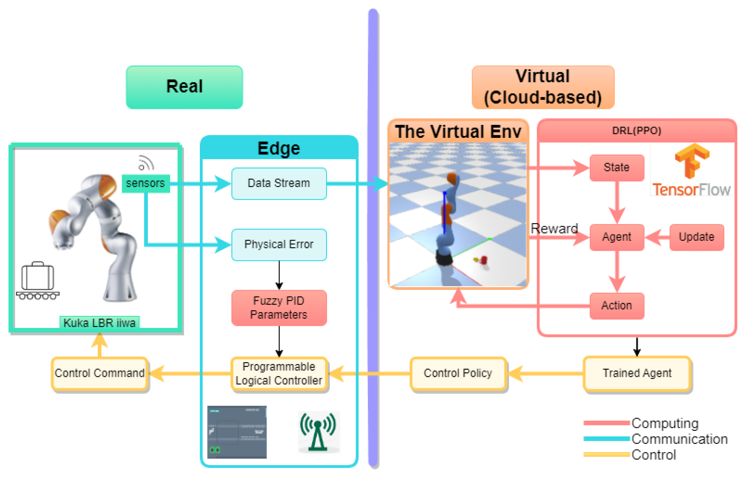
• Based on the IIoT environment, we propose a DT-empowered robotic arm control system. This system systematically elaborates the connections between the physical system and the control, communication, and computing subsystems. We also propose deploying computing tasks in the cloud to achieve decision-making and real-time control of the robotic arm, ensuring both safety and efficiency.
• We performed the kinematic analysis of the 6-degree-of-freedom robotic arm. We propose an integrated approach to achieve low-error control for the robotic arm. Specifically, for collision avoidance and trajectory planning, we developed a PPO-based adaptive control strategy. The PPO algorithm, deployed on the cloud computing center, serves as the primary decision-making mechanism. To further reduce errors following the algorithm’s decisions, we introduced a fuzzy PID controller at the device level. This controller was meticulously designed as an error compensation mechanism, forming a two-stage control framework that enhances the overall system’s precision and reliability.
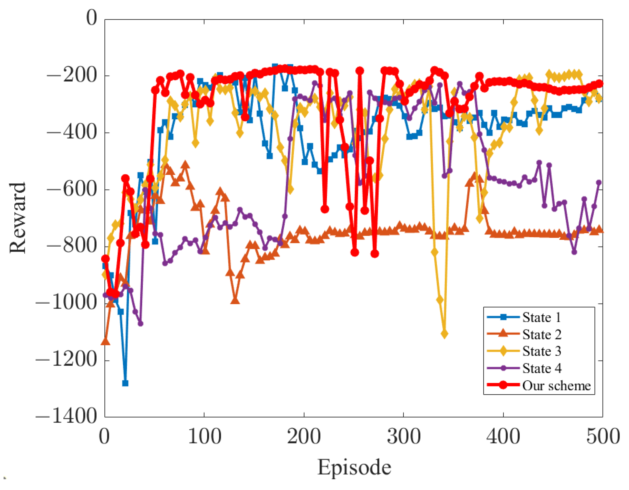
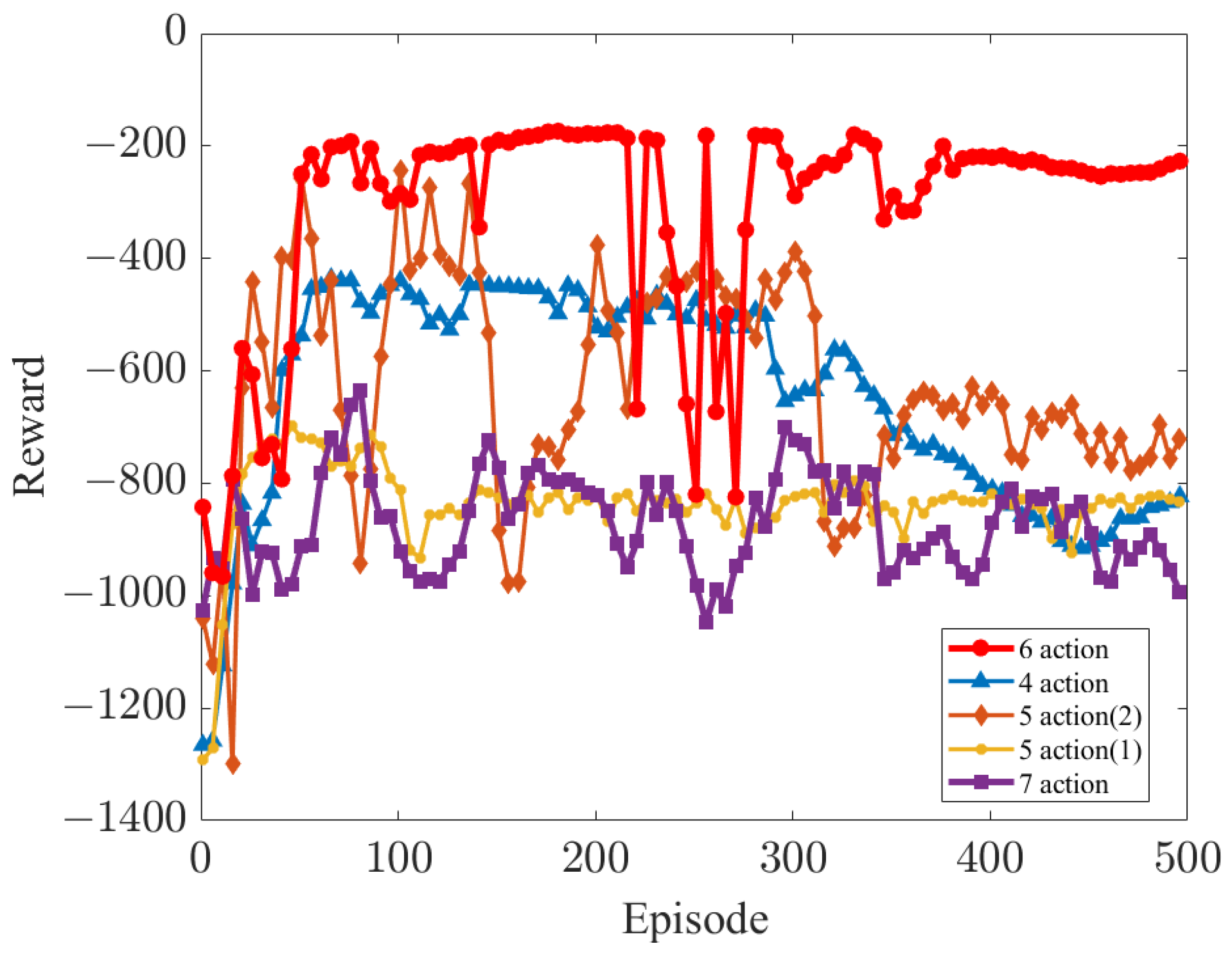
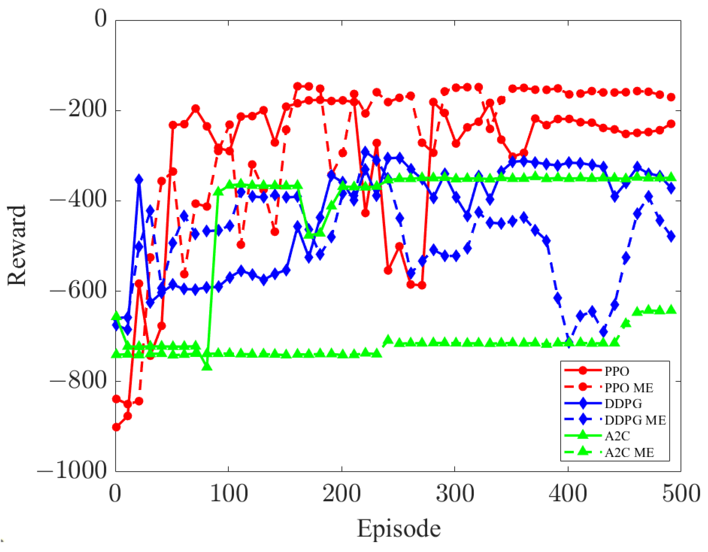
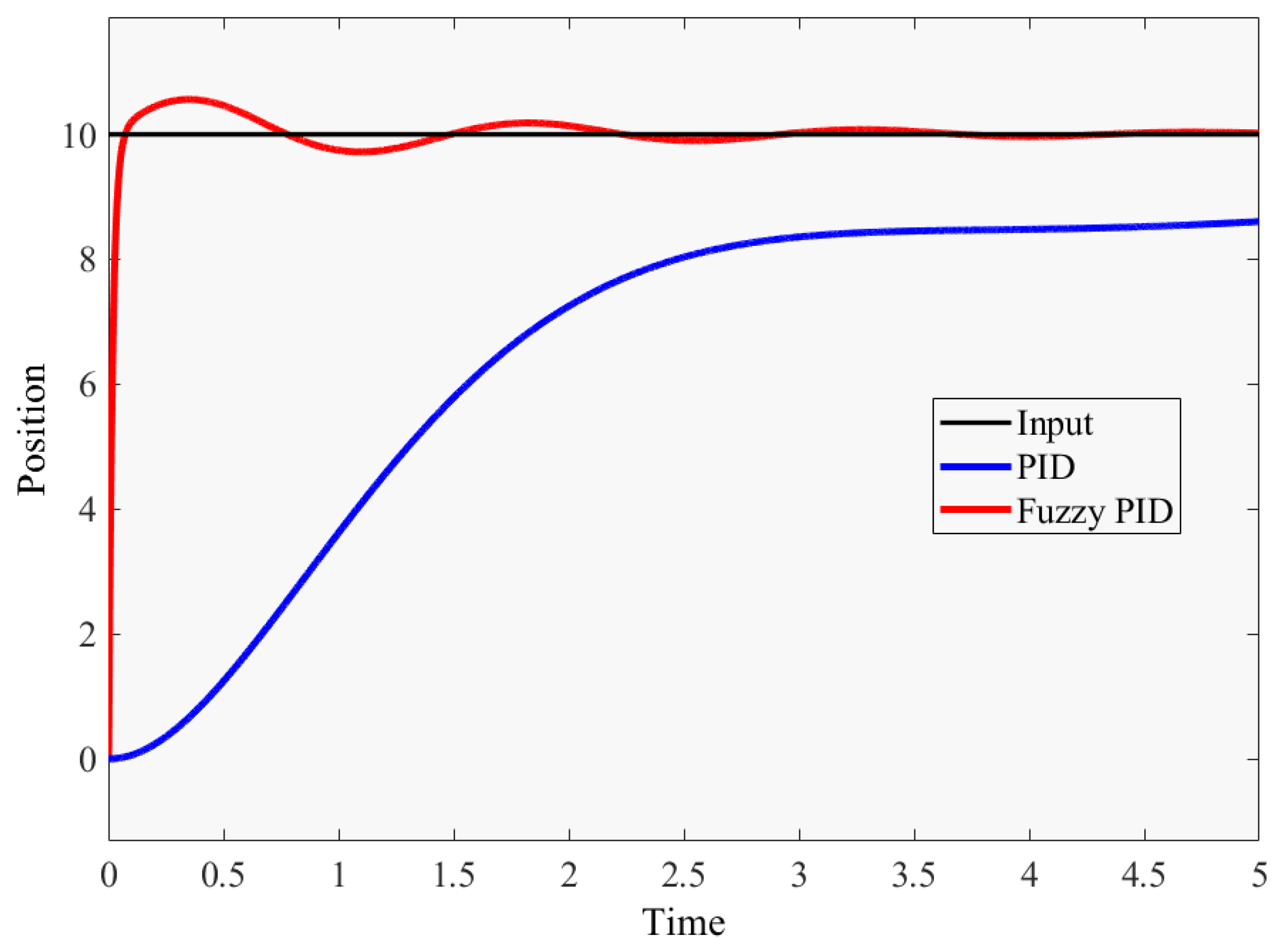
• In the simulation environment, we conducted experimental simulations to validate the effectiveness of the robotic arm control algorithms employed in the proposed DT system. The advantages of PPO as a decision algorithm are verified by comparing different schemes and baselines. At the same time, the advantages of fuzzy PID controllers are verified by comparing the performance with general PID controllers. The results show the performance and robustness of the integrated approach and also show its performance in mapping and execution error elimination.

The remainder of this article is organized as follows. In Section 2, we review the literature relevant to our problem. In Section 3, we provide the DT-empowered robotic arm control system and problem space and formalization. In Section 4, we present our approach, an integrated PPO and fuzzy PID approach, and the system implementation. In Section 5, we present the experimental simulations and performance evaluation. Finally, we present our conclusion and future work in Section 6.

2. Literature Review

This section reviews the related works in the construction and operations of the robotic arm control based on the DT framework. We review the control strategy of the robotic arms, including artificial intelligence methods and the classical control algorithms.

Recently, the application of DT in industrial process control and robotic arm systems has attracted attention due to its advantages such as real-time operation, data visualization, and remote collaboration. Bratchikov et al. [8] proposed the basic principles of DT design for robotic arms, describing the motion trajectories analytically or through motion quaternionic analysis. Ye et al. [24] developed a three-dimensional, real-time visualization monitoring and feedback system for the customized automatic transverse robot. This system, based on a data-driven DT system, realizes the failure prediction function. Yang et al. [25] constructed the kinematic analysis and actuator control models and realized the virtual–physical mapping and the remote motion interaction based on the DT framework. Park et al. [26] proposed a novel method to enhance the control performance of a degraded robotic arm by leveraging DT and the PPO algorithm. In general, the DT framework can be applied to robotic arms for monitoring and fault detection, and can also derive real-time and adaptive control strategies from the data-driven framework and additional computing power. However, the construction and operational design of DT systems based on the IIoT framework are still limited, and most research on DT systems for robotic arms remains conceptual, lacking practical industrial applications. The deployment and application of advanced algorithms within the DT framework are worth discussing.

There are also related studies on solving robot control strategies based on RL or DRL methods, whether they are based on simulation or reality environments. To reduce the difference between the simulation environment and the real environment, Joshi et al. [27] proposed a visual servoing mechanism that observes the scene and uses a double deep Q-learning framework, along with a novel grasp Q-Network, to output grasp probabilities. These probabilities are used to learn grasps that maximize pick success. Culter et al. [28] proposed a framework to search for the optimal control policy with fewer expensive real-world samples. Li et al. [29] developed a goal-conditioned self-imitation reinforcement learning method for robotic arm control in flexible flat cable assembly tasks. Their approach integrates hindsight and self-imitation learning modules to enable the robotic arm to optimize behavior planning and enhance exploration efficiency. Bing et al. [30] addressed challenges in robotic arm manipulation tasks with dynamic obstacles by proposing a bounding-box-based hindsight goal-generation method. This approach leverages image observations to dynamically generate intermediate goals, overcoming the limitations of graph-based methods in dynamic environments and improving exploration efficiency and task success rates. With DT technology, it is more effective to solve a control policy for the robotic arm in the simulation environment and deploy the policy to the physical robotic arm. Marius et al. [31] constructed a DT system for robotic arms, wherein the policies obtained through PPO training effectively controlled the arm’s motion. Similarly, Tian et al. [32] employed DRL algorithms to achieve path planning for a fruit-picking robot within a DT framework. Ren et al. [33] proposed a continuous learning strategy for the robotic arm grasp pose detection within the DT framework and a synthetic grasp detection dataset composed of industrial parts in the DT system. Most related works only focused on the DT system construction for the robotic arms and the control algorithms deployments and applications in the virtual. However, a critical challenge in DT applications is managing discrepancies between the virtual model and real-world operations. These modeling errors are often overlooked, leading to suboptimal control performance and reduced reliability in real-world scenarios. How to apply a suitable algorithm to search for the control strategy and avoid the ME is worth discussing.

A PID controller is widely used in robotic arm applications, and a fuzzy PID controller has demonstrated better performance. Huang and Yasonubu proposed a general practical design for a fuzzy PID and proved its performance to be better than conventional PID control [34]. Zhang et al. [35] detected and analyzed uncertain conditions, parameter delay, and interference in humanoid robotic arm control, to carry out fuzzy reasoning and perform online self-tuning of PID parameters. El-katib et al. [36] tested a 2-DOF PID controller and a fuzzy logic controller on a 4-DOF robotic arm, showing that the fuzzy logic controller had a faster response and better rise time, thus indicating superior performance. This means that the fuzzy PID controller is effective at controlling complex objects with imprecise models. Compared with PID, it also has greater flexibility and improves the fault tolerance of the system. However, there is a lack of research on the source analysis and elimination of errors at the physical end of DT. Discussions on the deployment of control systems within DT frameworks are also lacking. For the control problem of industrial equipment, it is necessary to use the fuzzy PID method in the DT system to correct physical errors in real-time.

3. Digital Twin-Empowered Robotic Arm Control System

3.1. System Architecture

Based on the KUKA LBR iiwa 6-degree-of-freedom (DOF) robotic arm, we constructed a DT-empowered robotic arm control system. Figure 1 describes this robotic arm control system and the interaction between each subsystem. The real component is the physical object that the system maps and controls, including the robotic arm, the actuator that drives the robotic arm, and its working environment. The virtual component involves accurate and real-time mapping of the robotic arm through modeling and simulation. In the information layer, the sensor collects and processes data from the physical robotic arm in real-time, transmitting the data to the edge server and cloud-based on IIoT to ensure real-time mapping in the virtual environment.

The work in this system, including each subsystem, focuses on the control of the robotic arm. The data stream obtained through the sensor was first uploaded to the cloud through the edge server of the IIoT, and the virtual robot arm of the DT system was constructed in real-time in the cloud. The cloud of the IIoT had a large amount of computing power. Therefore, the control policy for the robotic arm was developed using DRL deployed by the virtual system, where it was also debugged. The control command of the physical robotic arm was obtained by the control policy, sent from the cloud to the edge server, and then transmitted to the actuator to drive each joint motor and move the robot arm. After the strategy was executed, the sensor measured the motion error of the robot arm and fed back the existing physical error to the fuzzy PID control subsystem deployed in real-time for the real-time PID parameter adjustment. The dynamic PID parameters were fed back to the actuator for quick error correction. Next, we will discuss the mathematical form of the control problem of the robotic arms.

3.2. Robotic Arm Control Problem Formalization

3.2.1. Forward Kinematics Analysis of the Robotic Arm

Motion planning requires the robot arm to independently plan trajectories and track and reach the target point in the environment. At the same time, during the movement process, the trajectory of the robot arm’s end-effector must not collide with obstacles, and the output trajectory should be guaranteed to have a certain precision, with any deviations being corrected independently.

Excluding the end component, the KUKA LBR iiwa has 6 DOF, and the condition for successful capture is that the end position of the robot arm coincides with the position of the target point.

Referring to references [37,38,39,40,41,42,43], we present the kinematic model of the robotic arm. Figure 2 shows the structure of the robotic arm. It has six rotational joints. We define the set of joints as $\mathcal{J}=\{1,2,3,\dots ,6\}$, with the index of the joints denoted by i, $i\in \mathcal{J}$. Therefore, ${\theta }_i$ denotes the joint angles, ${\alpha }_i$ denotes the angles between the rotational axes of the joints and the rotational axes of the previous joints, $L_i$ denotes the lengths of the connecting rods, $d_i$ denotes the offset of the connecting rod.

According to ${\theta }_i$ and ${\alpha }_i$, the position and attitude of the robotic arm can be calculated, which can be donated by a homogeneous transformation matrix T. Assuming that the rotation transformation matrix of the i joint is $T_i$, the forward kinematics model of the robotic arm is as follows:

$$T_i^{i-1}=\left[\begin{array}{cccc}cos\left({\theta }_{\mathrm{i}}\right)& -sin\left({\theta }_{\mathrm{i}}\right)cos\left({\alpha }_{\mathrm{i}}\right)& sin\left({\alpha }_{\mathrm{i}}\right)sin\left({\theta }_{\mathrm{i}}\right)& L_{i}cos\left({\theta }_{\mathrm{i}}\right)\\ sin\left({\theta }_{\mathrm{i}}\right)& cos\left({\theta }_{\mathrm{i}}\right)cos\left({\alpha }_{\mathrm{i}}\right)& -cos\left({\theta }_{\mathrm{i}}\right)sin\left({\alpha }_{\mathrm{i}}\right)& L_{i}sin\left({\theta }_{\mathrm{i}}\right)\\ 0& sin\left({\alpha }_{\mathrm{i}}\right)& cos\left({\alpha }_{\mathrm{i}}\right)& d_i\\ 0& 0& 0& 1\end{array}\right]$$

(1)

$$T_6^0=T_1^0{T}_2^1{T}_3^2{T}_4^3{T}_5^4{T}_6^5$$

(2)

$$T_i^{i-1}=Ro{t}^Z\left({\theta }_i\right)\times Tran{s}^Z\left(d_i\right)\times Tran{s}^X\left(L_i\right)\times Ro{t}^X\left({\alpha }_i\right)$$

(3)

$${\mathrm{Rot}}^{\mathrm{Z}}\left({\theta }_i\right)=\left[\begin{array}{cccc}cos\left({\theta }_i\right)& -sin\left({\theta }_i\right)& 0& 0\\ sin\left({\theta }_i\right)& cos\left({\theta }_i\right)& 0& 0\\ 0& 0& 1& 0\\ 0& 0& 0& 1\end{array}\right]$$

(4)

$${\mathrm{Trans}}^{\mathrm{Z}}\left(d_i\right)=\left[\begin{array}{cccc}1& 0& 0& 0\\ 0& 1& 0& 0\\ 0& 0& 1& d_i\\ 0& 0& 0& 1\end{array}\right]$$

(5)

$${\mathrm{Trans}}^{\mathrm{X}}\left(L_i\right)=\left[\begin{array}{cccc}1& 0& 0& L_i\\ 0& 1& 0& 0\\ 0& 0& 1& 0\\ 0& 0& 0& 1\end{array}\right]$$

(6)

$${\mathrm{Rot}}^{\mathrm{X}}\left({\alpha }_i\right)=\left[\begin{array}{cccc}1& 0& 0& 0\\ 0& cos\left({\alpha }_i\right)& -sin\left({\alpha }_i\right)& 0\\ 0& sin\left({\alpha }_i\right)& cos\left({\alpha }_i\right)& 0\\ 0& 0& 0& 1\end{array}\right]$$

(7)

where ${\mathrm{Rot}}^{\mathrm{Z}}\left({\theta }_i\right)$ denotes the rotation matrix for a rotation angle ${\theta }_i$ around the Z-axis, ${\mathrm{Rot}}^{\mathrm{X}}\left({\alpha }_i\right)$ denotes the rotation matrix for a rotation angle ${\alpha }_i$ around the X-axis, ${\mathrm{Trans}}^{\mathrm{Z}}\left(d_i\right)$ denotes the translation matrix for a translation distance d along the Z-axis, and ${\mathrm{Trans}}^{\mathrm{X}}\left(L_i\right)$ denotes the translation matrix for a translation distance $L_i$ along the X-axis. Therefore, the control of the position of the end of the robotic arm can be converted to the control of the rotation angle of the joints of the robotic arm.

Based on Equations (1)–(7), $T_6^0$ can be represented as follows:

$$T_6^0=\left[\begin{array}{cccc}{n}_x& o_x& a_x& p_x\\ n_y& o_y& a_y& p_y\\ n_z& o_z& a_z& p_z\\ 0& 0& 0& 1\end{array}\right]=\left[\begin{array}{cccc}{n}_x& o_x& a_x& x_6\\ n_y& o_y& a_y& y_6\\ n_z& o_z& a_z& z_6\\ 0& 0& 0& 1\end{array}\right]$$

(8)

where the n, o, and a coordinate axes constitute the coordinate system of the end of the robotic arm, and the first three elements of the first, second, and third rows represent the rotation parts of the end of the robotic arm along the x, y, and z directions, respectively. p describes the translation portion of the rotation matrix along the x, y, and z directions. Therefore, $p_x,p_y,p_z$ denote the corresponding values of the end of the robotic arm.

The control policy based on DRL involves forward kinematic planning, which enables the agent’s output actions to control the rotation angle of each joint of the robotic arm, that is, ${\theta }_i$, so the end of the robotic arm can reach the target point in the environment.

When the position of the end of the arm $(x_6,y_6,z_6)$ coincides with the position of the target point $(x_{tar},y_{tar},z_{tar})$, the task is finished. The distance between them is as follows:

$$\mathrm{dist}1=\sqrt{{\left(x_6-x_{tar}\right)}^2+{\left(y_6-y_{tar}\right)}^2+{(z_6-z_{tar})}^2}$$

(9)

Similarly, in motion, it is necessary to ensure that the end of the robotic arm will not collide with the obstacle. We define the coordinates of the obstacle as $(x_{obs},y_{obs},z_{obs})$, and the distance between the end of the robotic arm and the obstacle is as follows:

$$\mathrm{dist}2=\sqrt{{\left(x_6-x_{obs}\right)}^2+{\left(y_6-y_{obs}\right)}^2+{(z_6-z_{obs})}^2}$$

(10)

Therefore, in the control policy of the robotic arm, the motion trajectory constraint of the policy is as follows:

$$\underset{{\theta }_i}{min}dist1$$

(11)

subject to

$$dist1\le a$$

(12)

$$dist2\ge b$$

(13)

$$0\le {\theta }_i\le {\theta }_i^{max},i\in \mathcal{J}$$

(14)

where a and b are the ranges of the target and the obstacle. ${\theta }_i^{max}$ is the maximum angle that can be reached by rotation.

3.2.2. Inverse Kinematics Analysis of Robotic Arm

After the implementation of the control policy, there are still unavoidable errors. In the virtual component, the control policy feeds commands back to the real component so that the actuator drives the motor, and each joint of the robotic arm reaches $(x_i,y_i,z_i),i\in \mathcal{J}$. Where the goal positions are $(x_g,y_g,z_g),g\in \mathcal{J}$.

Based on the current position and the goal positions, we aim to solve for the angle differences, which can be denoted as $\Delta \theta =[\Delta {\theta }_1,\Delta {\theta }_2,\Delta {\theta }_3,\Delta {\theta }_4,\Delta {\theta }_5,and\Delta {\theta }_6]$. By converting positional errors into angular errors, these can be corrected using control methods. According to the forward kinematics calculations of the robot arm mentioned above, $T_i^0$ can be represented as follows:

$$T_i^0=\left[\begin{array}{cccc}{n}_x& o_x& a_x& x_i\\ n_y& o_y& a_y& y_i\\ n_z& o_z& a_z& z_i\\ 0& 0& 0& 1\end{array}\right]$$

(15)

Then, the Jacobi matrix is established to find the inverse. The joints of the KUKA LBR iiwa robotic arm all rotate; thus, we have the following:

$$J{a}_i=\left[\begin{array}{ccc}{z}_{i-1}& \times (P_i& P_{i-1})\\ & z_{i-1}\end{array}\right]$$

(16)

$$Ja=\left[\begin{array}{cccccc}J{a}_1& J{a}_2& J{a}_3& J{a}_4& J{a}_5& J{a}_6\end{array}\right]$$

(17)

where $z_{i-1}$ represents the first three elements of the third row of the forward kinematics transformation matrix $T_{i-1}^0$; $P_i$ and $P_{i-1}$ represent the first three elements of the fourth columns of $T_i^0$ and $T_{i-1}^0$, respectively.

Thus, we establish the correspondence between the joint angular velocity in the joint space and the end-effector velocity in the robotic arm workspace.

Then, each joint of the robotic arm position $(x_i,y_i,z_i)$ can be present by $p_i$. It can be calculated by integrating velocity over time. Based on Euler’s integration method, given an integral interval $\Delta t$, the joint positions at time $t_k$ are known, and given the velocity of the end $v=[{\dot{x}}_i,{\dot{y}}_i,{\dot{z}}_i]$, the joint positions at time $t_{k+1}=t_k+\Delta t$ can be achieved by the following:

$$p_i\left(t_{k+1}\right)=p_i\left(t_k\right)+v\left(t_k\right)\Delta t.$$

(18)

Based on differential kinematics, the motion of the end of the robotic arm in the base coordinate can be approximately equal to the superposition of the motions of the joints. It is assumed that the robot moves step by step from the initial position p to the target position $p^{\prime }$, and the step length of each step can be viewed as the derivative of the rotation angle $\Delta \theta$, denoted as $\dot{\theta }$. Moreover, $\dot{\theta }$ can be expressed as follows:

$$\dot{\theta }=J{a}^{-1}v,$$

(19)

$$\dot{\theta }=[\dot{{\theta }_1},\dot{{\theta }_2},\dot{{\theta }_3},\dot{{\theta }_4},\dot{{\theta }_5},\dot{{\theta }_6}].$$

(20)

In this way, we can calculate the desired velocity of the joints at the current moment, denoted as $\dot{\theta }$, to achieve precise control and positioning of the robotic arm, and complete the control task of moving the end of the robotic arm to the target position.

4. An Integrated PPO and Fuzzy PID Approach

In this section, we mainly discuss the integrated PPO and fuzzy PID approach, including the detailed algorithm principle of PPO and fuzzy PID and the specific design for robotic arm control. Then, we discuss the specific workflow and pseudocode of the integrated approach. Finally, the computational complexity analysis of this integrated approach is given.

4.1. PPO Algorithm Design

PPO is a DRL algorithm based on the actor–critic framework. The robotic arm moves in three-dimensional space and actually faces a continuous control problem. The PPO algorithm can satisfy the need for continuous control, and it has good performance and stability for this control problem, so we use PPO as the training algorithm for the robotic arm control.

4.1.1. PPO Algorithm Principle

When using the PPO algorithm to address the continuous control problem within the actor–critic framework, the actor outputs an action, $a_t$, when the agent is at time step t while the state is $s_t$. The $a_t$ is sampled from the policy, which aims to satisfy the reward in state $s_t$. Define the mapping $\pi :S_t\to A_t$, where $\pi$ represents the policy, and $\pi \left(a\right|s)=P[A_t=a|S_t=s]$, with P denoting the probability of selecting action a given state s. The critic network evaluates the expected return and, upon inputting $s_t$, outputs the corresponding value $v_t$. This enables the agent to improve the action selection over iterations, leading to better rewards.

Based on importance sampling, PPO samples the old policy and updates the current policy on this basis. While at t, the policy is denoted as $\pi \left(a_t\right|s_t)$, and the past policy is denoted as ${\pi }_{old}\left(a_t\right|s_t)$. During iterations, the ratio between the two policies is as follows:

$$w_t\left(\phi \right)={\displaystyle \frac{\pi \left(a_t\right|s_t)}{{\pi }_{old}\left(a_t\right|s_t)}}.$$

(21)

However, the difference between the two policies may be significant, which can lead to a large deviation in the evaluation. Therefore, the distribution of the new and old policies should be constrained to make them more similar, ensuring a more accurate evaluation. In this paper, we adopt the PPO-Clip approach, where the loss function $Los{s}^{CLIP}\left(\phi \right)$ is as follows:

$$Los{s}^{CLIP}\left(\phi \right)=min(w_t\left(\phi \right)\widehat{A_t},clip(w_t\left(\phi \right),1-ϵ,1+ϵ))\widehat{A_t}$$

(22)

$$\widehat{A_t}=-V\left(s_t\right)+r_t+\gamma r_{(t+1)}+\dots +{\gamma }^{(T-t)}V\left(s_T\right)$$

(23)

where t is the time index in the trajectory segment $[0,T]$. $ϵ$ is the clip factor, in our approach, $ϵ=0.2$, and $\widehat{A_t}$ is the advantage function, which is used as the value evaluation of the current policy. $r_t$ represents the reward feedback to the agent at time step t. $V\left(s_t\right)$ is the output of the critic network, and $\gamma$ denotes the discount factor, which means that newer decisions are more important in memory. Meanwhile, in the implementation of importance sampling, two actor networks need to be built: one is used to output and iteratively update policies, while another, known as the old actor network, serves to store and record the old policy after an iteration and performs the $w_t\left(\phi \right)$ calculation. The Adam algorithm is used to update the actor and critic networks via stochastic gradient descent.

4.1.2. State and Action Spaces Definitions

In this paper, the problem to be solved involves controlling the output action of each joint to make the end of the robotic arm reach the target. Therefore, the action space is defined as the angular velocity of the six joints of the robotic arm, as follows:

$$action={\dot{\theta }}_i,\forall i\in \mathcal{J}$$

(24)

Similarly, the design of the observation space and the selection of state vectors in DRL significantly influence the rationality of the policy and the convergence speed of the algorithm. Therefore, we select vectors that are relevant to the task, such as the real-time parameters of the robotic arm, the positions of obstacles and targets, and the parameters of the observation space, as shown in

Table 1. Observation space $S_t$.

Parameters	Descriptions
$(x_i,y_i,z_i),i\in \{3\dots 6\}$	The position of each joint
$x_i-x_{tar},i\in \{3\dots 6\}$	The distance between the target and each joint in the X-axis direction
$y_i-y_{tar},i\in \{3\dots 6\}$	The distance between the target and each joint in the Y-axis direction
$z_i-z_{tar},i\in \{3\dots 6\}$	The distance between the target and each joint in the Z-axis direction
${\dot{\theta }}_i,i\in \mathcal{J}$	The velocity of each joint
$dist1$	The distance between the end and the target
$dist2$	The distance between the end and the obstacle
$\mathrm{indicator}$	Boolean algebra, indicating whether the target has been reached
$(x_{obs},y_{obs},z_{obs})$	The position of the obstacle
$(x_{tar},y_{tar},z_{tar})$	The position of the target
$x_6-x_{obs},y_6-y_{obs},z_6-z_{obs}$	The distances between the obstacle and the end in the X,Y and Z-axis direction

.

To prevent gradient disappearance and explosion during the neural network calculation process, and to eliminate anomalous data while complying with the calculation methods of neural networks, Z-score normalization processing of input variables is also performed.

4.1.3. Collision Detection and Reward Function

In this task, the objective is for the end of the robotic arm to reach the target area. Moreover, the robotic arm must not collide with the obstacle during its movement.

When the end of the robotic arm is in the range of the obstacle, the reward at time t is defined as follows:

$$r_{t1}=-\tau ,\tau >0, \mathrm{if}dist2\le b$$

(25)

where $\tau$ is a constant, and a large value is chosen in order to give a large penalty in the event of a collision between the robotic arm and an obstacle.

To guide the agent to control the end of the robotic arm toward the target, the reward $r_{t2}$ is as follows:

$$r_{t2}=-dist1.$$

(26)

And when the end of the arm is in the range of the target, positive feedback is given so that the end stays there. Thus, the reward $r_{t3}$ is expressed as follows:

$$r_{t3}=\delta ,\delta >0, \mathrm{if}dist1<a$$

(27)

where $\delta$ is also a constant. Therefore, the reward at time t can be defined as follows:

$$r_t=r_{t1}+r_{t2}+r_{t3}$$

(28)

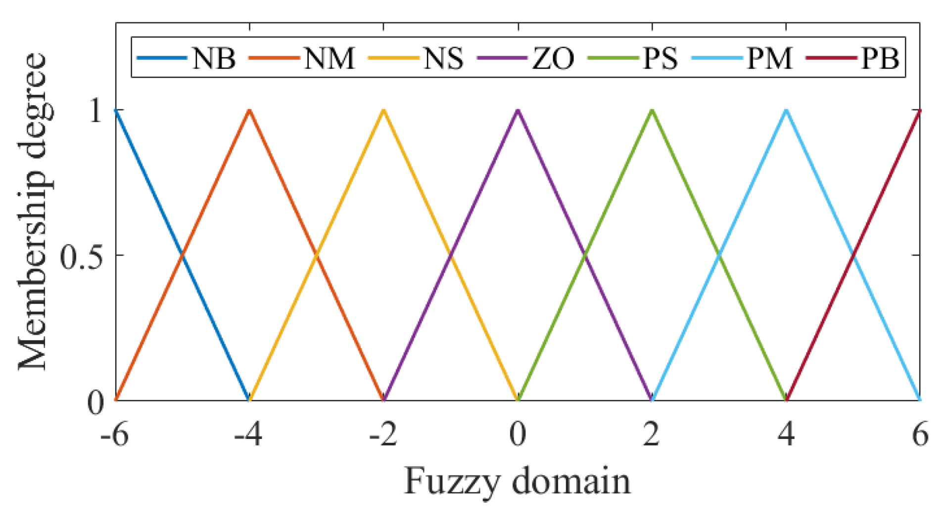
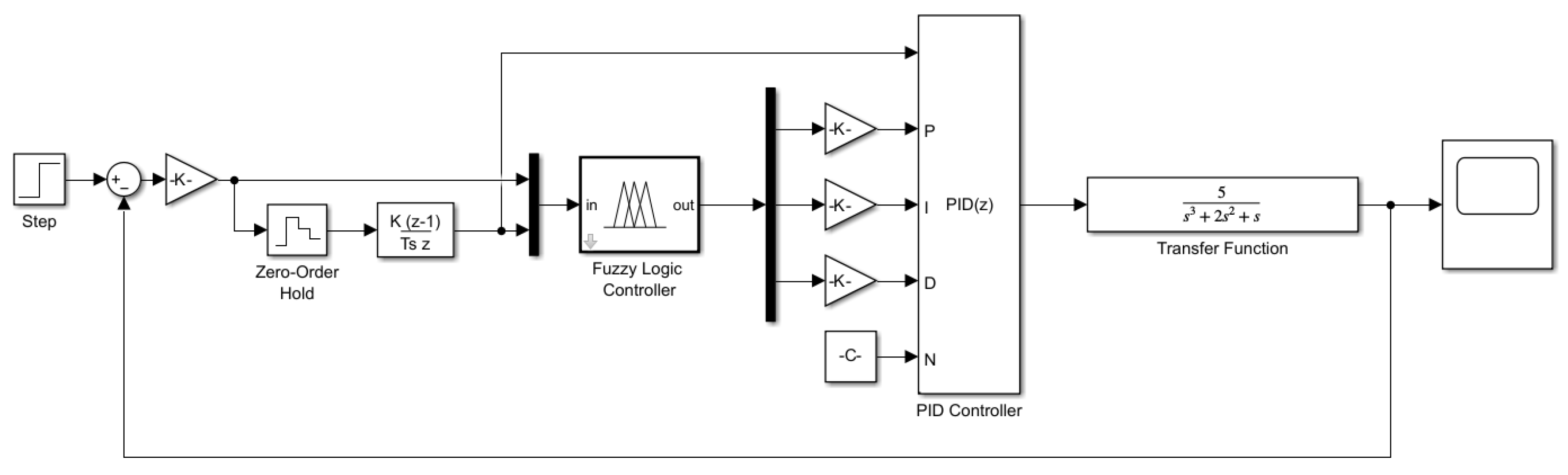
4.2. Fuzzy PID Control Design

Considering the errors in the physical system, PID control is often used to correct them. Compared to conventional PID control, we use fuzzy PID control, which offers improved performance. The key difference is that fuzzy PID can adjust the parameters in real-time, making them more suitable for the proportional–integral–derivative process.

In a continuous control system, given the input value $h\left(t\right)$, the form of the general PID is as follows:

$$u\left(t\right)=K_{p}e\left(t\right)+K_i{\int }_0^{t}e\left(t\right)dt+K_d{\displaystyle \frac{de\left(t\right)}{dt}}$$

(29)

$$e\left(t\right)=h\left(t\right)-u\left(t\right)$$

(30)

where $u\left(t\right)$ is the output of the PID controller, $e\left(t\right)$ is the error between the given value and the measured value, and ${\displaystyle \frac{de\left(t\right)}{dt}}$ can be denoted as $\dot{e}\left(t\right)$, which represents the error variation of $e\left(t\right)$. And $K_p$, $K_i$, $K_d$ are the PID controller parameters.

The fuzzy PID controller includes the fuzzy controller and PID controller, where the fuzzy controller takes the error $e\left(t\right)$ and error variation $\dot{e}\left(t\right)$ as input, and the PID parameters $K_p$, $K_i$, $K_d$ as output.

$$u\left(t\right)=K_{p}e\left(t\right)+K_i\sum _0^{t}e\left(t\right)+K_d(e\left(t\right)-e(t-1))=K_{p}e\left(t\right)+K_i\sum _0^{t}e\left(t\right)+K_d\dot{e}\left(t\right)$$

(31)

The first deals with fuzzification, where e is the angle error of each joint of the robotic arm, and the error variation in angle is denoted as $\dot{e}$. Moreover, e and $\dot{e}$ are the input linguistic variables, $K_p,K_i,K_d$ are the output linguistic variables, and their corresponding ranges of the fuzzy domains are as follows:

$$e,\dot{e},K_p,K_i,K_d=\{-6,-5,-4,-3,-2,-1,0,1,2,3,4,5,6\}.$$

(32)

For any measured physical signals, there exists a range for e and $\dot{e}$, denoted as $[V_{min},V_{max}]$. The task of fuzzification is to convert the continuous quantity between $[V_{min},V_{max}]$ and $[-6,6]$. By employing linear quantization, the function can be expressed as follows:

$$F\left(e\right)={\displaystyle \frac{12}{V_{max}-V_{min}}}(e-{\displaystyle \frac{V_{min}+V_{max}}{2}})$$

(33)

$$F\left(\dot{e}\right)={\displaystyle \frac{12}{V_{max}-V_{min}}}(\dot{e}-{\displaystyle \frac{V_{min}+V_{max}}{2}}).$$

(34)

The fuzzy membership functions are defined as follows:

$$e=\{NB,NM,NS,ZO,PS,PM,PB\}$$

(35)

$$\dot{e}=\{NB,NM,NS,ZO,PS,PM,PB\}$$

(36)

where the terms represent “negative big”, “negative middle”, “negative small”, “zero”, “positive small”, “positive middle”, and “positive big”, respectively. Their corresponding values are approximately $-6,-4,-2,0,2,4,6$. The fuzzy membership functions are the triangular membership functions, as shown in Figure 3.

Next, fuzzy rules for the proportional, integral, and derivative actions are established based on the PID control process. To illustrate, consider the time-domain analysis of a second-order system. The stages are defined as follows: the initial stage refers to the time before the rise time, the middle stage covers the period from the rise time to the setting time, and the later stage corresponds to the period after the setting time. In the initial stage of system regulation, a large $K_p$ value is necessary to achieve a fast response. As the regulation progresses to the middle stage, a smaller $K_p$ value is desired to minimize overshoot and maintain system stability. In the later stage of the adjustment process, increasing the $K_p$ value can help reduce static error and improve control accuracy. The integral gain $K_i$ should be adjusted to increase over time to continuously enhance the role of integration. This approach eliminates any steady-state error and improves control accuracy as time progresses. The $K_d$ is related to the inertia of the system. In the early stage of regulation, enhancing the function of differentiation improves the system’s initial response speed. In the middle stage, it is important to ensure the stability of the $K_d$ value to avoid introducing unnecessary oscillations or instability. Finally, in the later stage, reducing the function of differentiation helps accelerate convergence and achieve smoother final adjustments. Referring to [44],

Table 2. Fuzzy rules of $K_p$, $K_i$, $K_d$.

	e	NB	NM	NS	ZO	PS	PM	PB
$\dot{\mathit{e}}$
NB		PB ZO PS	PB ZO PS	PB ZO PS	PB ZO PS	PB ZO PS	PB ZO PS	PB ZO PS
NM		PB PS PS	PB PS PS	PM ZO PM	PM ZO PM	PM ZO PM	PM PS PS	PM PS PS
NS		PM PB PM	PM PB PM	PM ZO PM	PM ZO PM	PM ZO PM	PM PB PM	PM PB PM
ZO		PS PB PB	PS PB PB	ZO PB PB	ZO PB PB	ZO PB PB	PS PB PB	PS PB PB
PS		PM PB PM	PM PB PM	PS PM PB	PS PM PB	PS PM PB	PM PB PM	PM PB PM
PM		PB PS PS	PB PS PS	PM ZO PM	PM ZO PM	PM ZO PM	PB PS PS	PB PS PS
PB		PB ZO PS	PB ZO PS	PB ZO PS	PB ZO PS	PB ZO PS	PB ZO PS	PB ZO PS

Notes: Each cell contains three control rules, representing $K_p$, $K_i$, and $K_d$.

shows the fuzzy rules of $K_p$, $K_i$, $K_d$.

Performing fuzzy inference involves matching the input fuzzy quantity with the fuzzy rule base to obtain a set of fuzzy logic outputs, corresponding to each gain.

Finally, we have the work of defuzzification. This converts logical values to exact values. Based on the centroid method, the output can be calculated as follows:

$$K={\displaystyle \frac{{\sum }_i^n{M}_i{F}_i}{{\sum }_i^n{M}_i}}$$

(37)

where K is the exact value of the fuzzy controller output, $F_i$ is the fuzzy quantization value (for example, the value size corresponding to PB and ZO), and $M_i$ is the membership degree corresponding to $F_i$.

$K_p$, $K_i$, and $K_d$ values are constantly calculated, and these three parameter values are input into the PID controller to realize the automatic update of the $K_p$, $K_i$, and $K_d$ values, to realize the precise control of the robotic arm based on the fuzzy PID control.

4.3. The Integrated Approach Design

In summary, we propose the integrated PPO and fuzzy PID approach for robotic arm motion planning and execution. It includes two steps. First, based on the historical data and the virtual environment of the DT system, the PPO-Clip algorithm is used to train the agent. This computing task is deployed at the virtual end of the cloud computing center. The strategy is adaptive and can make reasonable decisions in changing environments and tasks. Then, the strategy is deployed to the real physical robotic arm and outputs actions to finish the task. After the motion execution, the robotic arm’s built-in functionality can detect errors in motion execution and target positioning, based on kinematic analysis or sensors. Finally, the fuzzy PID controller in real-time performs corrective actions, and the robotic arm reaches the target. The main algorithmic procedure is presented in Algorithm 1.

The error problem in the system is solved by applying the two-stage optimization algorithm of the virtual and real sides. At the same time, the system effectively uses the computing resources at the end and in the cloud.

Algorithm 1 An integrated PPO and fuzzy PID approach.

Require: Epoch $t_{ep}$, max time steps $t_{max}$, discount factor $\gamma$, actor network parameters ${\phi }^{Actor}$, critic network parameters ${\phi }^{Critic}$, actor learning rate $\alpha$, critic learning rate $\beta$;     for $i=1:t_{ep}$ do         for $j=1:t_{max}$ do             Get DT system state $s_t$;             Input $s_t$ to actor ${\phi }^{Actor}$ and get output $\mu$, $\sigma$;             Get the Gaussian distribution from $\mu$ and $\sigma$ as the policy $\pi \left(a_t\right|s_t)$;             Select action $a_t$ from the policy $\pi \left(a_t\right|s_t)$;             Store $\{s_t,a_t,r_t,s_{t+1}\}$ in the buffer;             if j % m == 0 then                 Select 10 random samples;                 Compute $Los{s}^{CLIP}\left(\phi \right)$ and update ${\phi }^{Actor}$ by (21)–(23);                 Compute loss function based on the critic output $v\left(s_t\right)$ and discounted reward;                 Update ${\phi }^{Critic}$ based on the loss function;             end if         end for     end for Ensure: The trained agent parameter ${\phi }^{Actor}$;     Send control commands based on the trained agent to the Real;     Execute control commands on the robotic arm;     Measure the physical error of the robotic arm by the sensor; Require: Error $e_i$, error variation ${\dot{e}}_i$;     for $i=1:6$ do         Fuzzing e and $\dot{e}$;         Compute $K_p$, $K_i$, $K_d$ based on (32)–(37);         Send parameters to the controller;         Perform fuzzy PID control at the i joint motor;     end for Ensure: The robotic arm reaches the target.

4.4. Algorithm Complexity Analysis

The PPO-Clip method contains the actor and critic networks. The layers that define the network of actors and critics are ${\zeta }^{Actor}$ and ${\zeta }^{Critic}$. The number of neurons at layer i of the actor network is denoted as ${\eta }_i$, and the number of neurons at layer j of the critic network is denoted as ${\eta }_j$. Thus, the total complexities of the actor and critic are as follows:

$${Cp}^{Actor}=O(\sum _{i=2}^{{\zeta }^{Actor}-1}({\eta }_{i-1}{\eta }_i+{\eta }_i{\eta }_{i+1})),$$

(38)

$${Cp}^{Critic}=O(\sum _{j=2}^{{\zeta }^{Critic}-1}({\eta }_{j-1}{\eta }_j+{\eta }_j{\eta }_{j+1})).$$

(39)

The training epoch is $t_{ep}$, and there are $t_{max}$ time steps in each epoch. When the m batch size is accumulated, it is updated once. Each time, 10 samples are selected to update $\kappa$ times. Thus, the total complexity of the PPO-Clip is as follows:

$${Cp}^{PPO}={\displaystyle \frac{10\kappa t_{ep}{t}_{max}}{m}}({Cp}^{Actor}+{Cp}^{Critic}).$$

(40)

In the process of fuzzy PID control, the computational tasks to be completed are fuzzification, fuzzy inference, and defuzzification. The fuzzification step involves transforming continuous input signals into fuzzy sets and has a complexity of $O\left(n\right)$, where n is the number of fuzzy sets used for error and change of error. The fuzzy inference step evaluates a rule base that contains $n^2$ rules. This results in a time complexity of $O\left(n^2\right)$ for the inference process. Finally, the defuzzification process, which uses the centroid method, requires a summation over the fuzzy output set. The complexity of this operation is $O\left(M\right)$, where M is the number of discrete points used in the calculation of the centroid. Thus, the computational complexity of each output of fuzzy PID is $O\left(n^2\right)$.

Assume that the control time of the fuzzy PID controller is $t_c$, and the sampling period is $t_{sam}$. In each sampling period, the controller outputs three parameters, $K_p$, $K_i$, and $K_d$. Therefore, the total computational complexity of the fuzzy PID controller is as follows:

$$C{p}^{Fuzzy}={\displaystyle \frac{3t_c}{t_{sam}}}O\left(n^2\right).$$

(41)

Therefore, the total computational complexity of the integrated approach is as follows:

$$C{p}^{total}={Cp}^{PPO}+C{p}^{Fuzzy}$$

(42)

5. Simulation and Performance Evaluation

In this section, we discuss the simulation experiments and performance analysis of the integrated approach for the robotic arm control. First, we build a robotic arm training environment to evaluate the performance of the PPO-Clip method. Based on different baselines and comparison schemes, we demonstrate the effectiveness of the PPO-Clip method for robotic arm control and its performance advantages in the ME environment. Then, we build the fuzzy PID controller simulation model and verify its performance on normal control objects.

5.1. Experiments Setting

We evaluate the realizability and performance of our proposed integrated PPO and fuzzy PID approach. The proposed control scheme is compared with other general schemes by first verifying the performance of the PPO algorithm in controlling the manipulator. Figure 4 shows the training environment of the robotic arm controlled by DRL algorithms. This verification is conducted within a robot simulation environment built using PyBullet. Within this environment, a red object serves as the target, while a yellow object is an obstacle. The goal is for the robotic arm to both reach the target and navigate around the obstacle. Both the positions of the obstacle and target are fixed, and the obstacle presents interference with the target object. We will also discuss and conduct simulation experiments from three aspects—state input selection, action control, and algorithm selection—to verify the advantages and rationality of our designed PPO control algorithm.

Table 3. State input schemes comparison.

Schemes	Descriptions
“state 1”	Without the positions of joints 3–5
“state 2”	Without all distance calculation information
“state 3”	Without the distances between joints 3 and 6 and the target
“state 4”	Without Z-score normalization

shows the contrasting state input schemes. “state 1”, “state 2”, and “state 3” lack information from some joints or adequate data processing. And the “state 4” scheme lacks Z-score normalization.

Table 4. Action control scheme comparison.

Schemes	Enable Moving Joints
“6 action”	Joints 1–6
“5 action (1)”	Joints 1–4, Joint 6
“5 action (2)”	Joint 1, Joint 2, Joints 4–6
“4 action”	Joint 1, Joint 2, Joint 4, Joint 6
“7 action”	All joints

lists different action control schemes, all of which can reach the target.

To verify the effect of ME on agent training. We choose the mainstream DRL algorithms for training within an environment that incorporates these errors. The objective is to observe and evaluate the adaptability of each algorithm to such errors. Therefore, random Gaussian noise is introduced to the state input vector, and the standard deviation of this noise is set at 5% of the absolute value of the state input. Furthermore, a comparative experiment is conducted involving the deep deterministic policy gradients (DDPGs), advantage actor–critic (A2C), and PPO.

Table 5. Parameter defaults of PPO.

Parameter	Value
Actor network structure	[512, 512, 256]
Critic network structure	[512, 512, 256]
Actor learning rate $\alpha$	$5\times {10}^{-5}$
Critic learning rate $\beta$	$1.5\times {10}^{-4}$
PPO clip value $ϵ$	0.2
Batch size	32
Time steps t	1000
Epoch $ep$	500
Target reaching detection a	0.2
Collision detection b	0.1
Discount factor $\gamma$	0.93

shows the relevant parameters of the PPO approach.

After executing the control commands issued by the agent, the physical errors in the system need to be corrected. Based on Matlab/Simulink, we built a fuzzy PID control model. Figure 5 shows the system simulation model. Firstly, the input values of fuzzy logic controllers e and $\dot{e}$ are obtained via the discretization of the system input and the introduction of a zero-order holder. Then, the fuzzy logic controller outputs the parameters $K_p,K_i,K_d$, after the gain input to the PID controller, and finally, the PID controller completes the control task. Depending on the structure and parameters of the robotic arm, the transfer function of the joint motor is a second-order or third-order system. Therefore, we select a second-order system and a third-order system, representing the system transfer function of a joint motor, to verify the performance of the fuzzy PID control, and compare it with the PID control of the given parameters.

Table 6. Parameter defaults for the fuzzy PID controller.

Parameter	Value	Descriptions
$K_i^2$, $K_p^2$, $K_d^2$	3.629, 3.533, 0.893	Given PID parameters in the second-order system
$K_i^3$, $K_p^3$, $K_d^3$	0.169, 0.003, 2.090	Given PID parameters in the third-order system
$h^2\left(t\right)$	1	System input in the second-order system
$h^3\left(t\right)$	10	System input in the third-order system

shows the parameter settings of the PID control simulations.

The second-order transfer function is as follows:

$$\begin{array}{c}\hfill G\left(s\right)={\displaystyle \frac{1}{s^2+2s+1}}\end{array}$$

And the third-order transfer function is as follows:

$$\begin{array}{c}\hfill G\left(s\right)={\displaystyle \frac{5}{s^3+2s^2+s}}\end{array}$$

5.2. Performance Evaluation

The experimental results confirm that the PPO algorithm effectively addresses the challenges of robotic arm motion planning and obstacle avoidance. The output optimal policy is relatively simple and direct, and it can converge quickly in calculations. The large amount of data and computational resources provided by the DT platform can be used to quickly realize the control of industrial robotic arms with virtual–real interactions.

Figure 6 shows that among the various state input vector selection schemes, the scheme we designed can reach convergence the fastest, and the output reward is the smoothest after convergence. The cumulative reward increased rapidly in the early training period, fluctuated in the middle of the training period as the agent continued to explore environmental interactions, attempted to touch obstacles, and then stabilized at a high level in the late training period. The cumulative reward of reaching around −200 for each epoch is represented by the ability to reach the target point in the least number of time steps at the time of action output (without negotiating with the obstacle(. Regarding the performance of other schemes—“state 1” lacks the information input of other joints of the robotic arm; although it can fulfill the task requirements, the output reward fluctuates a lot and is lower compared to the state input we selected ($S_t$). Moreover, “state 2” only inputs the basic target distance and obstacle distance, which cannot converge at all; “state 3” lacks the distance calculation of each joint coordinate of the robotic arm and the target coordinate, so the output reward fluctuates greatly and the result is not smooth. And “state 4” suffers from the largest reward fluctuations due to the lack of normalization processing, making the calculation of the neural network difficult.

Figure 7 shows that the optimal control policy is achieved when six joints are controlled, resulting in the agent receiving a larger reward compared to other control schemes, and allowing for stable convergence. Moreover, “5 action (1)” and “7 action” are not able to accomplish the target task and receive less reward throughout the training period, making convergence difficult. The control schemes based on “4 action” and “5 action (2)” instead become worse in the later stages of training, fluctuate more, and fail to accomplish the target task. In summary, our control scheme can obtain an optimal policy in robotic arm motion planning and control tasks using the PPO algorithm.

Figure 8 shows the comparison of the performance of DRL algorithms with the virtual–real ME. The curriculum reward of the PPO with ME is not much different from the original PPO. This means that PPO has good adaptability to noise, its performance is almost the same as that in the noiseless environment, and the policy output in the noisy environment can also complete the task. A2C cannot complete the training task in an environment with noise, and its performance is much worse in an environment without ME. The performance of DDPG is also worse than that of PPO, and its policy lacks stability in the environment with ME. In general, PPO outperforms the other baselines in the normal environment. Meanwhile, in the ME environment, PPO shows the smallest drop in performance. Therefore, in the DT system with the virtual–real ME, deploying PPO is an ideal choice, PPO can effectively use the data with errors and obtain the required policies.

In the second-order and third-order systems, fuzzy PID control has better performance than the normal PID control, the response time of fuzzy PID is shorter, the overshoot is lower than the PID control with given parameters, and the adjustment time is faster. For the same second-order and third-order systems, fuzzy PID control is more stable than ordinary PID control, and can adjust errors faster and more accurately to meet the performance required for the precise control of the robot arm. Figure 9 and Figure 10 show the results.

6. Conclusions

In this paper, we propose an integrated industrial robotic arm control system that combines DT technologies, DRL algorithms, fuzzy mathematics methods, and a PID controller. This system integrates communication, control, and computing within the framework of IIoT and its reliability and effectiveness have been verified. To eliminate the errors in the DT system, this paper presents an integrated PPO and fuzzy PID control approach to mitigate these errors. By using the data provided by the DT system, PPO is applied to training, combined with fuzzy PID control to eliminate errors. This remote collaboration and control method significantly improves efficiency compared to traditional teaching methods. And the integrated approach performs well in error management. It not only eliminates the errors in the DT system but also handles them with relatively high efficiency.

References

1. Alshamaa, D.; Cherubini, A.; Passama, R.; Pla, S.; Damm, L.; Ramdani, S. RobCap: A Mobile Motion Capture System Mounted on a Robotic Arm. IEEE Sens. J. 2022, 22, 917–925. [Google Scholar] [CrossRef]
2. Hirzinger, G.; Bals, J.; Otter, M.; Stelter, J. The DLR-KUKA Success Story: Robotics Research Improves Industrial Robots. IEEE Robot. Autom. Mag. 2005, 12, 16–23. [Google Scholar] [CrossRef]
3. Liu, S.; Liu, P. A Review of Motion Planning Algorithms for Robotic Arm Systems. In Proceedings of the 8th International Conference on Robot Intelligence Technology and Applications (RiTA); Springer: Singapore, 2021; pp. 56–66. [Google Scholar]
4. Zheng, K.; Luo, R.; Liu, X.; Qiu, J.; Liu, J. Distributed DDPG-Based Resource Allocation for Age of Information Minimization in Mobile Wireless-Powered Internet of Things. IEEE Internet Things J. 2024, 11, 29102–29115. [Google Scholar] [CrossRef]
5. Yang, L.-Y.; Chen, S.-Y.; Wang, X.; Zhang, J.; Wang, C.-H. Digital Twins and Parallel Systems: State of the Art, Comparisons, and Prospect. Acta Autom. Sin. 2019, 45, 2001–2031. [Google Scholar]
6. Haag, S.; Anderl, R. Digital Twin-Proof of Concept. Manuf. Lett. 2018, 15, 64–66. [Google Scholar] [CrossRef]
7. Minerva, R.; Lee, G.M.; Crespi, N. Digital Twin in the IoT Context: A Survey on Technical Features, Scenarios, and Architectural Models. Proc. IEEE 2020, 108, 1785–1824. [Google Scholar] [CrossRef]
8. Bratchikov, S.; Abdullin, A.; Demidova, G.L.; Lukichev, D.V. Development of digital twin for robotic arm. In Proceedings of the IEEE 19th International Power Electronics and Motion Control Conference (PEMC), Gliwice, Poland, 25–29 April 2021; pp. 717–723. [Google Scholar]
9. Zeb, S.; Mahmood, A.; Hassan, S.A.; Piran, J.; Gidlund, M.; Guizani, M. Industrial digital twins at the nexus of nextG wireless networks and computational intelligence: A survey. J. Netw. Comput. Appl. 2022, 200, 103309. [Google Scholar] [CrossRef]
10. Cronrath, C.; Aderiani, A.R.; Lennartson, B. Enhancing digital twins through reinforcement learning. In Proceedings of the 2019 IEEE 15th International Conference on Automation Science and Engineering (CASE), Vancouver, BC, Canada, 22–26 August 2019; pp. 293–298. [Google Scholar]
11. Xia, K.; Sacco, C.; Kirkpatrick, M.; Saidy, C.; Nguyen, L.; Kircaliali, A.; Harik, R. A digital twin to train deep reinforcement learning agent for smart manufacturing plants: Environment, interfaces and intelligence. J. Manuf. Syst. 2021, 58, 210–230. [Google Scholar] [CrossRef]
12. Recht, B. A tour of reinforcement learning: The view from continuous control. Annu. Rev. Control Robot. Auton. Syst. 2019, 2, 253–279. [Google Scholar] [CrossRef]
13. Buşoniu, L.; de Bruin, T.; Tolić, D.; Kober, J.; Palunko, I. Reinforcement learning for control: Performance, stability, and deep approximators. Annu. Rev. Control 2018, 46, 8–28. [Google Scholar] [CrossRef]
14. Saravanan, M.; Kumar, P.S.; Sharma, A. IoT enabled indoor autonomous mobile robot using CNN and Q-learning. In Proceedings of the 2019 IEEE International Conference on Industry 4.0, Artificial Intelligence, and Communications Technology (IAICT), Bali, Indonesia, 1–3 July 2019; pp. 7–13. [Google Scholar]
15. Saroj, A.; Trant, T.V.; Guin, A.; Hunter, M.; Sartipi, M. Optimizing Traffic Controllers along the MLK Smart Corridor Using Reinforcement Learning and Digital Twin. In Proceedings of the 2022 IEEE 2nd International Conference on Digital Twins and Parallel Intelligence (DTPI), Boston, MA, USA, 24–28 October 2022; pp. 1–2. [Google Scholar]
16. Zhang, X.; Lyu, X.; Wang, T.; Huang, B. Research on decision control system of tunneling robot driven by digital twin. Coal Sci. Technol. 2022, 50, 36–49. [Google Scholar]
17. Wu, Z.; Yao, Y.; Liang, J.; Jiang, F.; Chen, S.; Zhang, S.; Yan, X. Digital twin-driven 3D position information mutuality and positioning error compensation for robotic arm. IEEE Sens. J. 2023, 99, 1. [Google Scholar] [CrossRef]
18. Jiang, F.; Ding, K.; He, G.; Sun, Y.; Wang, L. Vibration fault features of planetary gear train with cracks under time-varying flexible transfer functions. Mech. Mach. Theory 2021, 158, 104237. [Google Scholar] [CrossRef]
19. Schulman, J.; Wolski, F.; Dhariwal, P.; Radford, A.; Klimov, O. Proximal policy optimization algorithms. arXiv 2017, arXiv:1707.06347. [Google Scholar]
20. Miao, J.; Zheng, H.; Xie, Z.; Lai, J.; Jiang, L. Offloading Optimization in Digital Twin-Aided UAV Networks. J. Beijing Univ. Posts Commun. 2022, 45, 133–139. [Google Scholar]
21. Borase, R.P.; Maghade, D.K.; Sondkar, S.Y.; Pawar, S.N. A review of PID control, tuning methods and applications. Int. J. Dyn. Control 2021, 9, 818–827. [Google Scholar] [CrossRef]
22. Shah, P.; Agashe, S. Review of fractional PID controller. Mechatronics 2016, 38, 29–41. [Google Scholar] [CrossRef]
23. Kumar, V.; Nakra, B.C.; Mittal, A.P. A review on classical and fuzzy PID controllers. Int. J. Intell. Control Syst. 2011, 16, 170–181. [Google Scholar]
24. Ye, W.; Liu, X.; Zhao, X.; Fu, H.; Cai, Y.; Li, H. A Data-Driven Digital Twin Architecture for Failure Prediction of Customized Automatic Transverse Robot. IEEE Access 2024, 12, 59222–59235. [Google Scholar] [CrossRef]
25. Yang, H.; Cheng, F.; Li, H.; Zuo, Z. Design and Control of Digital Twin Systems Based on a Unit Level Wheeled Mobile Robot. IEEE Trans. Veh. Technol. 2024, 73, 323–332. [Google Scholar] [CrossRef]
26. Park, S.-Y.; Lee, C.; Kim, H.; Ahn, S.-H. Enhancement of Control Performance for Degraded Robot Manipulators Using Digital Twin and Proximal Policy Optimization. IEEE Access 2024, 12, 19569–19583. [Google Scholar] [CrossRef]
27. Joshi, S.; Kumra, S.; Sahin, F. Robotic Grasping using Deep Reinforcement Learning. In Proceedings of the 2020 IEEE 16th International Conference on Automation Science and Engineering (CASE), Hong Kong, China, 20–21 August 2020; pp. 1461–1466. [Google Scholar]
28. Cutler, M.; Walsh, T.J.; How, J.P. Real-World Reinforcement Learning via Multifidelity Simulators. IEEE Trans. Robot. 2015, 31, 655–671. [Google Scholar] [CrossRef]
29. Li, J.; Shi, H.; Hwang, K.-S. Using Goal-Conditioned Reinforcement Learning with Deep Imitation to Control Robot Arm in Flexible Flat Cable Assembly Task. IEEE Trans. Autom. Sci. Eng. 2024, 21, 6217–6228. [Google Scholar] [CrossRef]
30. Bing, Z.; Álvarez, E.; Cheng, L.; Morin, F.O.; Li, R.; Su, X. Robotic Manipulation in Dynamic Scenarios via Bounding-Box-Based Hindsight Goal Generation. IEEE Trans. Neural Netw. Learn. Syst. 2023, 34, 5037–5050. [Google Scholar] [CrossRef] [PubMed]
31. Matulis, M.; Harvey, C. A robot arm digital twin utilising reinforcement learning. Comput. Graph. 2021, 95, 106–114. [Google Scholar] [CrossRef]
32. Tian, X.; Pan, B.; Bai, L.; Wang, G.; Mo, D. Fruit Picking Robot Arm Training Solution Based on Reinforcement Learning in Digital Twin. J. ICT Stand. 2023, 11, 261–282. [Google Scholar] [CrossRef]
33. Ren, L.; Dong, J.; Huang, D.; Lü, J. Digital Twin Robotic System with Continuous Learning for Grasp Detection in Variable Scenes. IEEE Trans. Ind. Electron. 2024, 71, 7650–7660. [Google Scholar] [CrossRef]
34. Huang, Y.; Yasunobu, S. A general practical design method for fuzzy PID control from conventional PID control. In Proceedings of the Ninth IEEE International Conference on Fuzzy Systems. FUZZ-IEEE 2000 (Cat. No. 00CH37063), San Antonio, TX, USA, 7–10 May 2000; Volume 2, pp. 969–972. [Google Scholar]
35. Zhang, Y.; Sun, L.; Zhang, Y. Research on Algorithm of Humanoid Robot Arm Control System Based on Fuzzy PID Control. In Proceedings of the 2022 International Conference on Artificial Intelligence and Autonomous Robot Systems (AIARS), Bristol, UK, 29–31 July 2022; pp. 337–341. [Google Scholar]
36. El-Khatib, M.F.; Maged, S.A. Low level position control for 4-DOF arm robot using fuzzy logic controller and 2-DOF PID controller. In Proceedings of the 2021 International Mobile, Intelligent, and Ubiquitous Computing Conference (MIUCC), Cairo, Egypt, 26–27 May 2021; pp. 258–262. [Google Scholar]
37. Chen, S. Research on the Technology of Zero Moment Control and Collision Detection of Collaborative Robot. Ph.D. Dissertation, University of Science and Technology of China, Hefei, China, 2018. [Google Scholar]
38. Zhao, T.-J.; Yuan, J.; Zhao, M.-Y.; Tan, D.-L. Research on the Kinematics and Dynamics of a 7-DOF Arm of Humanoid Robot. In Proceedings of the 2006 IEEE International Conference on Robotics and Biomimetics, Kunming, China, 17–20 December 2006; pp. 1553–1558. [Google Scholar]
39. Nugroho, G.; Riyadi, A.F. Design and Repeatability Test of a 6 Degree of Freedom Robotic Arm. In Proceedings of the 2021 International Conference on Advanced Mechatronics, Intelligent Manufacture and Industrial Automation (ICAMIMIA), Surabaya, Indonesia, 8–9 December 2021; pp. 218–222. [Google Scholar]
40. Kofinas, N.; Orfanoudakis, E.; Lagoudakis, M.G. Complete analytical forward and inverse kinematics for the NAO humanoid robot. J. Intell. Robot. Syst. 2015, 77, 251–264. [Google Scholar] [CrossRef]
41. Singh, T.P.; Suresh, P.; Chandan, S. Forward and inverse kinematic analysis of robotic manipulators. Int. Res. J. Eng. Technol. (IRJET) 2017, 4, 1459–1468. [Google Scholar]
42. Mohammed, A.A.; Sunar, M. Kinematics modeling of a 4-DOF robotic arm. In Proceedings of the 2015 International Conference on Control, Automation and Robotics, Singapore, 20–22 May 2015; pp. 87–91. [Google Scholar]
43. Denavit, J.; Hartenberg, R.S. A Kinematic Notation for Lower-Pair Mechanisms Based on Matrices. J. Appl. Mech. 1955, 22, 215–221. [Google Scholar] [CrossRef]
44. Yang, Y.; Cui, D.; Zhou, A. Fuzzy adaptive PID controller and Simulink simulation. Ship Electron. Eng. 2010, 4, 127–130. [Google Scholar]
Figure 1. Digital twin-empowered robotic arm control system architecture.
Mathematics 13 00216 g001
Figure 2. The robotic arm simplified model.
Mathematics 13 00216 g002
Figure 3. Fuzzy membership functions.
Mathematics 13 00216 g003
Figure 4. DRL training environment by PyBullet.
Mathematics 13 00216 g004
Figure 5. System Simulation model by Matlab/Simulink.
Mathematics 13 00216 g005
Figure 6. Performance comparison of each state input scheme.
Mathematics 13 00216 g006
Figure 7. Performance comparison of each action control scheme.
Mathematics 13 00216 g007
Figure 8. Performance of mainstream DRL algorithms with mapping errors.
Mathematics 13 00216 g008
Figure 9. Fuzzy PID and PID controller response curve in the second-order system.
Mathematics 13 00216 g009
Figure 10. Fuzzy PID and PID controller response curve in the third-order system.
Mathematics 13 00216 g010