Abstract
This paper presents a Neural Network-Based Symbolic Computation Algorithm (NNSCA) for solving the (2+1)-dimensional Yu-Toda-Sasa-Fukuyama (YTSF) equation. By combining neural networks with symbolic computation, NNSCA bypasses traditional method limitations, deriving and visualizing exact solutions. It designs neural network architectures, converts the PDE into algebraic constraints via Maple, and forms a closed-loop solution process. NNSCA provides a general paradigm for high-dimensional nonlinear PDEs, showing great application potential.
Keywords:
neural network-based symbolic computation; (2+1)-dimensional YTSF equation; exact solutions; nonlinear partial differential equations MSC:
35A25; 68T07; 35Q51
1. Introduction
Nonlinear partial differential equations (NLPDEs) are fundamental to numerous fields in science and engineering due to their capacity to accurately characterize complex nonlinear phenomena inherent in both natural and artificial systems. These equations occupy a central position at the forefront of scientific and technological research, with widespread applications extending across fluid dynamics [1], quantum physics [2], ecology [3], optics [4], economics [5], and various other domains of mathematical physics. Determining exact solutions for such nonlinear equations represents a significant research direction within mathematical physics. Prominent examples include the Navier–Stokes equations in fluid dynamics [6], the Schrödinger equation in quantum mechanics [7], and the Korteweg–de Vries equation [8], all of which are inherently nonlinear. Deriving their exact solutions provides critical insights into intrinsic dynamical behaviors, stability conditions, and underlying complex patterns, such as soliton phenomena [9]. Furthermore, exact solutions are indispensable for understanding how system behavior depends on parameter variations. For instance, in power system modeling, the analysis of exact solutions to nonlinear synchronization equations elucidates the conditions under which self-organized synchronization occurs—an essential consideration in modern grids with increasing penetration of distributed energy resources [10]. Similarly, in crystal physics, exact solutions for anharmonic crystals enhance our understanding of heat transfer mechanisms and the relaxation dynamics of correlation functions [11].
In recent years, a growing number of methods have been developed for solving NLPDEs. Notable techniques include the Hirota bilinear method [12], the inverse scattering transform [13], the generalized exponential rational function method (GERF) [14], Lie symmetry analysis [15], and Darboux and Bäcklund transformations [16], among others. Each of these methods possesses distinct advantages and is suited to solving specific types of nonlinear partial differential equations.
The Yu-Toda-Sasa-Fukuyama (YTSF) equation is an important model in nonlinear science, describing wave propagation phenomena in various physical systems. These include interfacial waves in two-layer fluids and quasi-planar elastic waves in lattices [17]. Originally derived from the principle of strong symmetry, the YTSF equation plays a significant role in capturing essential features of nonlinear physical dynamics. In fluid dynamics, the YTSF equation models wave behavior at the interface between two fluid layers, with valuable applications in marine science and engineering—such as predicting wave propagation in shallow seas [18]. In plasma physics, it aids in understanding nonlinear wave dynamics, offering insights critical to nuclear fusion research and space physics. Additionally, the equation is closely linked to nonlinear optics and wave evolution in weakly dispersive media, thereby supporting advances in optical signal processing and fiber optic communications [19].
Significant research efforts have been dedicated to devising mathematical methods for constructing exact solutions to the YTSF equation and its variants, as these solutions are crucial for elucidating the equation’s rich dynamical properties. The Hirota bilinear method is a powerful tool for solving exact solutions of NLPDEs and is particularly suitable for the construction of soliton solutions. Foroutan et al. successfully applied this method to obtain a lump solution and five interaction solutions for (3+1) dimensional potential YTSF equations [20]. It simplifies the solution process by transforming the nonlinear equations into a bilinear form. Zhao et al. used Hirota’s bilinear method and the long-wave limit method to obtain a rich mixture of solutions for the (2+1)-dimensional YTSF equations, including the K-order lump, the L-breather, and the M-soliton solutions [21]. Huang et al. also established the M-soliton solution, the block solution, and the three types of interaction solutions for the (3+1)-dimensional YTSF-like equations by the Hirota bilinear method with the aid of Maple software [22]. Manafian et al. investigated the periodic wave solutions for the (3+1)-dimensional YTSF equations by this method [23]. Wang et al. systematically derived the multisoliton solutions of the (3+1)-dimensional Kadomtsev-Petviashvili-Yu-Toda-Sasa-Fukuyama (KP-YTSF) equation using Hirota’s bilinear method [24]. There are also other methods to solve the YTSF equations, such as Gandhi et al. obtained the exact solution of the YTSF equations with time-varying coefficients, including traveling wave solutions in the form of hyperbolic, rational, and trigonometric functions, using the generalized (G′/G) expansion method and the modified simplex method of equations (NMSEM) [25], which consists in converting the nonlinear partial The exact solutions are obtained by converting the nonlinear partial differential equations to ordinary differential equations by assuming that the solutions are functions that depend on the solutions of the auxiliary equations. Kumar et al. combined Lie symmetry analysis and the generalized Kudryashov (GK) method to obtain a wide range of exact soliton solutions and different dynamical waveforms for the (3+1)-dimensional YTSF equations [26]. But for different solutions, different methods are suitable for different types of nonlinear equations or different forms of the same equation. For example, some methods may be better at finding traveling wave solutions, while others are more suitable for finding non-traveling wave solutions or solutions containing arbitrary functions [27], some methods have strong assumption dependence and the solution space will be limited, for example, when solving the YTSF equation, the block solution (Lump solution) cannot be obtained by using the extended hyperbolic function method [28], and when using Hirota’s bilinear method, the reliance on the exponential superposition form can generate hybrid solutions, but the parameters need to be manually adjusted, which may miss the solution for complex nonlinear systems [29]. In addition, traditional methods for finding exact solutions to nonlinear partial differential equations are difficult to solve in high-dimensional or nonaccumulatable systems [30,31], so it is necessary to develop more general and efficient exact solution search methods.
In the last few years, the rapid development of Neural Network Method (NNM) has brought a new paradigm for solving nonlinear partial differential equations.The Universal Approximation Theorem proposed by Cybenko in 1989 [32] lays a theoretical foundation for neural networks to approximate any continuous function, which enables neural networks to effectively learn and represent complex nonlinear relationships. Raissi’s Physically Informed Neural Networks (PINNs) [33], which use the laws of physics as regularization terms for neural network training, are able to solve differential equations even with sparse or no data. However, the traditional PINN also has some challenges, such as difficulty in training complex multi-frequency patterns or steep gradient problems, and poor performance in three-dimensional problems and problems with discontinuous solutions [34], subsequent researchers have carried out a number of refinements and optimizations, such as Lu et al. developed the DeepXDE framework [35], which dynamically optimizes the training process through adaptive refinement strategies, thus improving computational efficiency and optimizing the training process. Wei et al. designed a multi-scale neural network (MscaleDNN) [36] to adapt multi-scale input features and enhance the ability of solving complex nonlinear partial differential equations, and Zhang innovatively fused the bilinear approach with neural networks and proposed a Bilinear Neural Network Method (BNNM) to solve complex nonlinear partial differential equations [37]. BNNM uses a bilinear structure adapted with a generalized approximation theorem, which enables it to efficiently generate nonlinear wave solutions such as solitons and respirators, which are of great importance in the fields of optics and fluid mechanics.
Compared to the existing PINN and BNNM, the novelty and effectiveness of Neural Network Based Symbolic Algorithm (NNSCA) are fully reflected. While PINN has strong function approximation capabilities, it requires reliance on automatic differentiation methods for calculations, which is very time-consuming for higher-order derivatives. This results in a lack of timeliness for PINN. Another issue is that PINN currently lacks effective optimization algorithms to train the network to reach optimal solutions. The limitation of BNNM lies in its high constraints on the equations being solved. It requires the equations to be integrable. Furthermore, the original equations must undergo a bilinear transformation before proceeding to the next step, but in reality, many equations cannot be subjected to bilinear transformation, which significantly detracts from the applicability of BNNM.
In terms of method architecture, NNSCA utilizes the structural a priori of symbolic derivation and the approximation advantage of neural networks, while integrating the complementary logics of symbolic computation and neural networks, which not only abandons the strong dependence of traditional symbolic methods such as Hirota on bilinear transformations, but also breaks through the black-box nature and the lack of physical meaning of the purely data-driven methods, and constructs a neural network exploring the solution space with a complex functional form, and a neural network exploring the solution space and symbolic computation constraints on the physical rigor of the closed loop, breaking the double barriers of the traditional framework and realizing a new paradigm for solving nonlinear partial differential equations with accurate solutions. Compared to traditional symbolic methods, NNSCA dramatically accelerates the derivation process for solving (2+1)-dimensional equations by automating the handling of parameter-constrained equations. Its iterative optimization approach requires minimal manual parameter tuning, significantly reducing the computational cost of complex solutions. This method lowers the entry barrier for users and establishes a novel paradigm for addressing high-dimensional fractional nonlinear PDEs. The new path is provided for the accurate solution of high-dimensional fractional-order nonlinear PDEs. Wang et al. [17]. derived the wave solution of the (2+1)-dimensional YTSF equation via symbolic computation; Zhao et al. investigated its Weierstrass elliptic function solution employing the traveling wave transformation [22]. Using the NNSCA, the (2+1)-dimensional YTSF equation was successfully solved for the first time, yielding a series of novel solutions. The obtained analytical solutions were visualized by means of three-dimensional surface plots, heat maps, and contour maps.
The (2+1) dimensional YTSF equation is shown in (1).
where is the potential function, which physically corresponds to the amplitude of the wave or the fluid velocity potential.
In this equation, three types of core terms are included that determine the complex dynamics of the wave. In the (2+1)-dimensional YTSF equation, is the nonlinear term, whose wave amplitude modulates nonlinearly on its own gradient, resulting in a steepening of the waveform. is the dispersion term, with fourth-order spatial derivatives describing the diffusion of the high-frequency components, which balances with the nonlinear term to maintain soliton stability. is the two-dimensional coupling term, the second-order derivative in the y-direction introduces transverse constraints that allow for localized Lump solutions and the existence of obliquely propagating solitons.
The rest of the paper is structured as follows: in Section 2, the principle of this neural network-based symbolic computation method and its overall process and steps for solving nonlinear partial differential equations will be introduced, and in Section 3, the analytical solution of the (2+1)-dimensional YTSF equation using the neural network-based symbolic computation method will be demonstrated using the two single hidden-layer neural network models designed as an example and its analytic solution will be visualized. In Section 4, the model complexity will be increased by taking the three double hidden layer neural network models designed as an example to solve the analytical solution of the (2+1) dimensional YTSF equation using the neural network based symbolic computation method and visualize its analytical solution. In Section 5, the conclusions of the study will be presented.
2. Principles of NNSCA
The development of the NNSCA method, as depicted in Figure 1, is inspired by both symbolic computation and the Bilinear Neural Network Method (BNNM). BNNM has proven effective in solving a range of nonlinear partial differential equations, including the (3+1)-dimensional Boiti–Leon–Manna–Pempinelli equation [38], the (3+1)-dimensional shallow water wave equation [39], the (2+1)-dimensional Konopelchenko–Dubrovsky–Kaup– Kupershmidt equation [40], the Hirota–Satsuma–Ito equation [41], the gBS-like equation [42], and the (3+1)-dimensional Jimbo–Miwa equation [43]. Unlike BNNM, the NNSCA method eliminates the need for bilinear transformation, significantly reducing the complexity of application and improving computational efficiency for high-dimensional nonlinear systems. The overall workflow of the proposed method is illustrated in Figure 1, with the detailed neural network architecture presented in Figure 2.
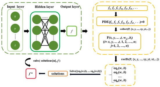
Figure 1.
NNSCA method flowchart.
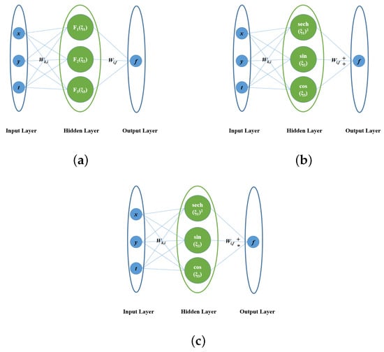
Figure 2.
Neural Networks Model of Signal Hidden layer: (a) Network Architecture. (b) Model [3-3-1]-1. (c) Model [3-3-1]-2.
The procedure consists of the following steps:
Step 1 Define the neural network architecture, as depicted in Figure 2 (single hidden layer) and Figure 5 (double hidden layer). A detailed description of the model structure is provided in subsequent sections.
Step 2 Express the solution to the nonlinear PDEs using the analytical form of the neural network.
Step 3 Substitute this expression into the target Equation (1) to formulate a system of algebraic equations.
Step 4 Extract the coefficients associated with the independent variables and their derivative terms to construct the system of algebraic equations to be solved.
Step 5 Solve the resulting algebraic system to obtain constraints solely on the weights (w) and biases (b).
Step 6 Incorporate these constraints into the neural network expression from Step 1 to derive an exact solution to the original PDE (1). Finally, validate the solution by substituting it back into the initial equation.
The primary principle guiding the selection and design of the neural network architecture follows a systematic, step-by-step progression from shallow to deep structures. For example, the architecture evolves from a single hidden layer to multiple hidden layers, with activation functions transitioning from additive coupling to a blend of additive and multiplicative interactions. This approach establishes a robust foundation for the subsequent development of the NNSCA. For single-hidden-layer networks, the model denoted as [3-3-1]-1 represents the initial architecture, comprising 3 input neurons, 3 hidden neurons, and 1 output neuron, as illustrated in Figure 2a. This model differs from Model [3-3-1]-2 primarily in the choice of activation function used in the hidden layer. Further details regarding these distinctions will be elaborated in subsequent sections.
Here, and denote the weights in the network transmission process, represents the bias coefficients, and Equation (2) provides a clear interpretation of the single hidden layer network model. Model [3-3-1]-2 is similar to [3-3-1]-1, with the only difference being that the accumulation algorithm is modified to a combination of addition and multiplication.
and denote the weights in the network transmission process, represents the bias coefficients, and Equation (3) provides a clear interpretation of the double hidden layer network model. Model [3-3-2-1]-3 is similar to [3-3-2-1]-1 and [3-3-2-1]-2, with the only difference being that the accumulation algorithm is modified to a combination of addition and multiplication.
3. Single Layer
3.1. Model [3-3-1]-1
In order to solve the (2+1)-dimensional Yu-Toda-Sasa-Fukuyama Equation (1), we can firstly choose a network model with a single hidden layer as shown in Figure 2a: where the input layer has three neurons, denoted as x, y and t, and the hidden layer has three neurons, denoted as , , and . And now respectively we make , , , to get the model as shown in Figure 2b. According to this neural network model we can get the expression Equation (4).
Differentiating and substituting Equation (4) back into Equation (1) yields nine solutions by NNSCA, one of which is as follows
Substituting Equation (5) into Equation (4) gives the final solution of the original equation as
the final solution Equation (6) is also visualized, as shown in Figure 3a–d.
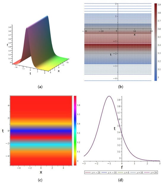
Figure 3.
Bright Soliton Solution (6) to the (2+1)-dimensional YTSF eauation: (a) Three-dimensional graphs. (b) Contour diagrams. (c) Thermal maps. (d) Evolution plot.
governs the temporal scaling of soliton pulse width Figure 3d. dictates the oblique propagation angle Figure 3b. denotes the baseline field potential in the absence of wave excitation.
- Three-dimensional graphs Figure 3a: A single-peak localized 3D structure is observed, with f forming a soliton-type peak in the spatiotemporal domain (smooth decay in all directions). The dispersion term suppresses peak spreading, while the nonlinear term drives steepening; their balance maintains soliton localization (finite-area distribution) and stability (no waveform spreading/morphology conservation).
- Contour diagrams Figure 3b: Oblique bright bands (intertwined with gradient colors) correspond to oblique traveling wave solutions, varying monotonically with the x, t coupling direction. This verifies the spatio-temporal translational invariance (morphological repetition along propagation), supported by linear dispersion.
- Thermal maps Figure 3c: Symmetric color distribution (low center, high edge) reflects x, t plane symmetry constraints, embodying spatio-temporal symmetry and energy diffusion characteristics of this 2D nonlinear wave.
- Evolution plot Figure 3d: A single-peaked curve (uniform f, t-only variation) represents a time-domain soliton/pulse solution, reflecting transient energy concentration from nonlinear focusing and verifying time-locality and morphological stability.
3.2. Model [3-3-1]-2
To obtain distinct analytical solutions for neural network models with the same number of layers, we keep the number of layers in the network model unchanged and modify the operation symbol between the hidden layer and the output layer. The original weighted sum form is transformed into a combined form of weighted sums and products, yielding the model [3-3-1]-2 shown in Figure 2c. This model explicitly defines the operational logic for aggregating the hidden layer outputs into output layer converting implicit connections into explicit operations. Based on this neural network model, we derive Expression Equation (7).
Differentiating Equation (7) and substituting back into Equation (1) yields 17 solutions by NNSCA, one of which is as follows
Substituting Equation (8) into Equation (7) and simplifying gives the final solution of the original equation as
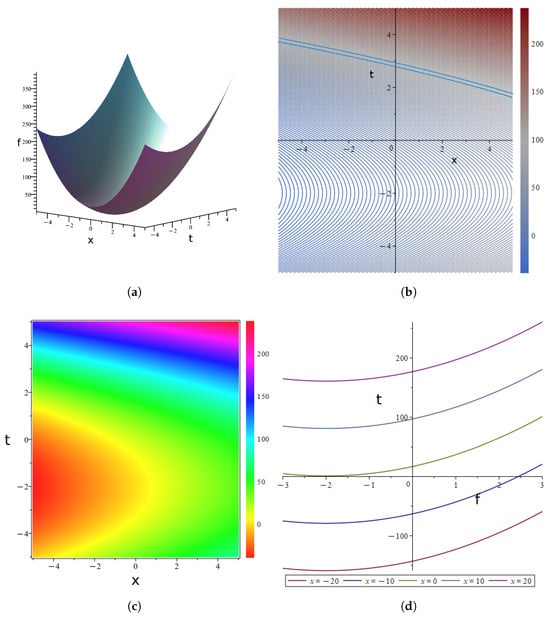
Figure 4.
Parametric Rational Solution (9) to the (2+1)-dimensional YTSF eauation: (a) Three-dimensional graphs. (b) Contour diagrams. (c) Thermal maps. (d) Evolution plot.
mediates transverse gradient symmetry Figure 4c symmetry axis. scales the nonlinear-dispersion balance strength sustaining soliton stability. determines the growth rate of the quadratic background field.
- Three-dimensional graphs Figure 4a: The figure presents the double - sheet laminar soliton structure of the exact solution to the (2+1)-dimensional YTSFequation. f constructs two independent localized spatiotemporal planes, corresponding to the 2D double-soliton solutions. The solitons remain unfused and have stable morphologies, reflecting the locality (finite-domain distribution) and stability (non-spreading waveforms) of solitons in nonlinear equations. Neural networks can fit their nonlinear mappings, and symbolic computation can derive analytical solutions, collaboratively revealing the formation mechanism and dynamic essence of the soliton structure.
- Contour diagrams Figure 4b: Features dense interleaved oblique contour lines, corresponding to oblique traveling wave solutions. Spatial variation with in the coupling direction reflects spatio-temporal translational invariance, driven by a balance between linear dispersion and nonlinear terms.
- Thermal maps Figure 4c: Displays oblique symmetric color gradients (symmetric about the origin), representing 2D symmetric oblique traveling waves. The center-to-edge gradient reflects spatial energy diffusion, verifying the spatio-temporal symmetry and energy locality of the (2+1)-dimensional solution.
- Evolution plot Figure 4d: Different colored curves correspond to fixed values of x (), showing the evolution of f over time. Neural networks fit non-linear trends, and symbolic computation ensures the analytical structure. Together, they collaboratively reconstruct the complex spatiotemporal dynamics of the equation. The variation in curve shapes with x reflects the spatio-temporal coupling driven by nonlinear terms, which validates the effectiveness of the combined method in revealing the behavior of the equation.
4. Double Layer
4.1. Model [3-3-2-1]-1
In order to verify the upgrade from ad hoc solution to generalization of the methodology, we now increase the complexity of the model to solve the (2+1)-dimensional YTSF equation (Equation (1)) by constructing a double hidden layer, as shown in the model [3-3-2-1] in Figure 5a: where the input layer has three neurons denoted as , and t; the first hidden layer contains three neurons, denoted as , , and , where , , ; the second hidden layer contains two neurons, denoted as , , where , . At this point, we obtain the neural network model [3-3-2-1] shown in Figure 5b. According to the neural network model, we can get the expression Equation (10).
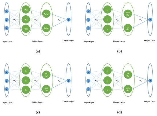
Figure 5.
Neural Networks of Doublue Hidden Layers Model. (a) Network Architecture. (b) Model [3-3-2-1]-1. (c) Model [3-3-2-1]-2. (d) Model [3-3-2-1]-3.
Differentiating and substituting Equation (10) back into Equation (1) yields eight solutions by NNSCA, one of which is as follows
Substituting Equation (11) into Equation (10) gives the final solution of the original equation as
acts as a characteristic frequency scaling factor (Figure 6b) stripe periodicity. modulates hyperbolic saturation intensity. controls oscillatory amplitude in the trigonometric component.
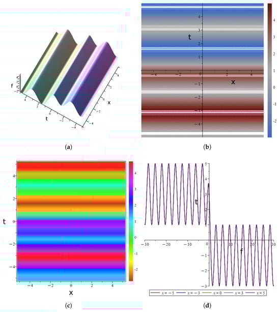
Figure 6.
Linearly Coupled System Solution (12) to the (2+1)-dimensional YTSF eauation: (a) Three-dimensional graphs. (b) Contour diagrams. (c) Thermal maps. (d) Evolution plot.
- Three-dimensional graphs Figure 6a: Displays a double-sheet laminar structure, representing a 2D space-time double-soliton solution. The balance between non-linearity and dispersion maintains localization and stability of the solitons.
- Contour diagrams Figure 6b: Features dense horizontal stripes, corresponding to traveling wave solutions. Verifies spatial-temporal translational invariance, driven by the coupling of linear dispersion and nonlinearity.
- Thermal maps Figure 6c: Shows alternating horizontal color bands, exhibiting spatio-temporal periodic oscillations, dominated by the resonance between nonlinearity and dispersion.
- Evolution plot Figure 6d: Presents a single-peaked pulse (spatially uniform), a time-domain soliton pulse solution. Transient energy concentration arises from nonlinear focusing.
4.2. Model [3-3-2-1]-2
In order to get different analytical solutions in the double hidden layer of the neural network, according to Figure 5 (the [3-3-2-1] model), we adjust the second hidden layer (while keeping the input layer and the first hidden layer unchanged): the hyperbolic tangent function in the second hidden layer is replaced by a sinusoidal function, and the cosine function is replaced by a hyperbolic secant function, i.e., and . This modified second hidden layer forms the [3-3-2-1]-2 neural network model shown in Figure 5c, leading to the expression Equation (13).
Differentiating Equation (13) and substituting it back into Equation (1) yields seven solutions via NNSCA, one of which is
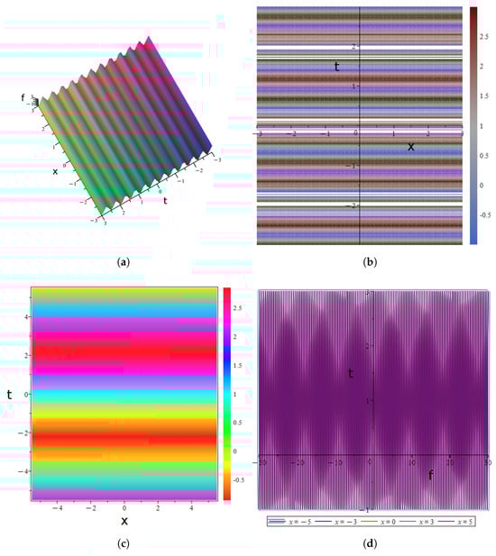
Figure 7.
Periodic Wave Solution (15) to the (2+1)-dimensional YTSF eauation: (a) Three-dimensional graphs. (b) Contour diagrams. (c) Thermal maps. (d) Evolution plot.
- Three-dimensional graphs Figure 7a: Displays a double-sheet laminar structure, where f forms two independent localized surfaces. This embodies 2D space-time double soliton solutions, with the balance between nonlinearity and dispersion maintaining soliton localization and stability.
- Contour diagrams Figure 7b: Features dense horizontal stripes, corresponding to equiphase surfaces of traveling wave solutions. It verifies spatio-temporal translational invariance, driven by the coupling of linear dispersion and nonlinearity.
- Thermal maps Figure 7c: Shows alternating horizontal color bands, exhibiting spatio-temporal periodic oscillations of f. This reflects the resonance effect between nonlinearity and dispersion.
- Evolution plot Figure 7d: Presents a single-peaked pulse shape with uniform spatial x, representing a time-domain soliton pulse solution. Nonlinear focusing dominates the transient energy concentration.
4.3. Model [3-3-2-1]-3
In order to obtain different analytical solutions for the neural network model with the same layer count, we modify the operation between the hidden layer and output layer in the second field (while keeping the network layer structure unchanged) for the model [3-3-2-1]-2: replacing the original weighted sum with a product. This yields the model [3-3-2-1]-3 (shown in Figure 5d), where the operation relationship during the aggregation of hidden layer outputs to f is explicitly defined (shifting from “implicit connection” to “explicit operational logic”). Based on this model, we derive the expression Equation (14).
Differentiating Equation (16) and substituting it back into Equation (1) yields 10 solutions via NNSCA, one of which is
The Multi-Soliton Solution is visualized in Figure 8, corresponding to Three-dimensional graphs, Contour diagrams, Thermal maps and Evolution plot. regulates inter-soliton spacing in coupled structures (Figure 8a double-lobe separation). The product defines the fundamental oscillation frequency. quantifies the intensity of phase-dependent nonlinear interactions.
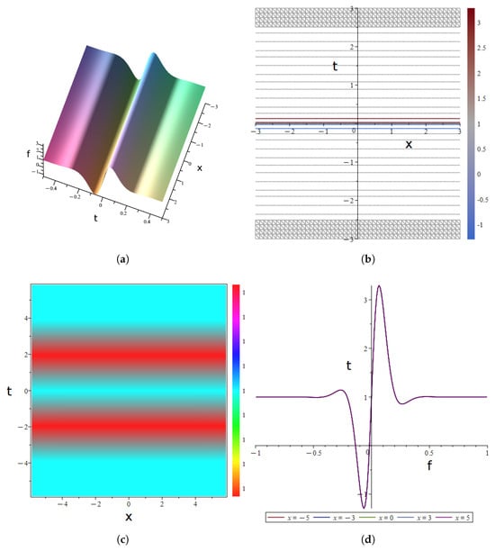
Figure 8.
Multi-Soliton Solution (18) to the (2+1)-dimensional YTSF eauation: (a) Three-dimensional graphs. (b) Contour diagrams. (c) Thermal maps. (d) Evolution plot.
- Three-dimensional graphs Figure 8a: Exhibits a double-lobed localized structure, representing a 2D space-time coupled soliton solution. Nonlinearity-dispersion balance sustains soliton locality and stability.
- Contour diagrams Figure 8b: Displays dense diagonal stripes, corresponding to oblique traveling wave solutions. Verifies spatio-temporal translational invariance, driven by linear-nonlinear coupling.
- Thermal maps Figure 8c: Shows horizontal color band oscillations, reflecting spatio-temporal periodicity. Dominated by nonlinear-dispersive resonance.
- Evolution plot Figure 8d: Presents a single-peaked pulse (spatially uniform), a time-domain soliton. Nonlinear focusing induces transient energy concentration.
5. Conclusions
The NNSCA method, introduced in this paper, innovatively integrates neural networks with symbolic computation. It establishes a novel paradigm for tackling high-dimensional nonlinear partial differential equations. The approach shows significant promise. It has been validated for the first time on the (2+1)-dimensional YTSF equation. The NNSCA method revolutionizes solution space exploration. It transcends traditional frameworks and seamlessly integrates neural networks with symbolic computation. Five specialized neural network types are designed to address the two-dimensional coupling in the (2+1)-dimensional YTSF equations. This approach eliminates reliance on bilinear transformations, such as Hirota’s method constraints, and directly explores the solution’s function space. It overcomes limitations of accumulable systems. Symbolic-differential constraints ensure mathematical rigor in the network’s output. Compared with traditional methods, NNSCA synergistically improves efficiency and universality. numerical methods rely on initial values and discretization introduces errors, NNSCA directly outputs analytical solutions, eliminates discretization errors, and adapts to arbitrary initial value exploration. BNNM require bilinear transformation preprocessing and their solution types are limited, while NNSCA has no preprocessing step and autonomously learns complex structures such as Lump-soliton hybrid solutions.
The NNSCA method offers greater generalizability than PINNs. It requires less computational power. This stems from their distinct solution approaches. PINNs rely on deep neural networks’ universal approximation properties to construct solution spaces. They embed PDE residuals as physical constraints in the loss function for joint optimization. This yields an explicit functional form of the solution. However, this process demands significant computing resources. In contrast, NNSCA integrates symbolically derived structural priors with neural network approximation. It solves exact PDE solutions and verifies them through backtesting. NNSCA excels in both solution accuracy and computational efficiency. Currently, NNSCA has efficiently solved the (2+1)-dimensional YTSF equations, but when extended to (3+1)-dimensional or fractional-order PDEs, the complexity of network parameters and symbolic computation still needs to be optimized. Future research will aim to extend the NNSCA method to higher-dimensional problems. It will also target other partial differential equation families, such as fractional-order PDEs. Structural optimization remains a key focus. This includes designing multi-branch hidden layers. Adaptive activation function libraries will be developed. These enhancements will address high-dimensional equations with variable coefficients.
Author Contributions
Conceptualization, J.-L.S. and R.-F.Z., methodology, J.-L.S., validation, J.-L.S. and R.-F.Z., writing—original draft preparation, J.-L.S., J.-W.H. and J.-B.L., writing—review and editing, J.-L.S., supervision, J.-L.S. and R.-F.Z., project administration, J.-L.S., funding acquisition, J.-L.S. and R.-F.Z. All authors have read and agreed to the published version of the manuscript.
Funding
This research was funded by Yibin University grant number. ‘2024XJPY13’ and Tianyuan Fund for Mathematics of the National Natural Science Foundation of China. ‘12426105’ and Fundamental Research Program of Shanxi Province. ‘202403021222001’ and Open Foundation of Hubei Key Laboratory of Applied Mathematics (Hubei University). ‘HBAM202401’ and the Wen Ying Young Scholars Talent Project of Shanxi University ‘138541088’ and The APC was funded by Yibin University ‘2024XJPY13’.
Data Availability Statement
No new data were created or analyzed in this study.
Conflicts of Interest
The authors declare no conflicts of interest.
References
- Min, E.-H.; Koo, W.; Kim, M.-H. Wave Characteristics over a Dual Porous Submerged Breakwater Using a Fully Nonlinear Numerical Wave Tank with a Porous Domain. J. Mar. Sci. Eng. 2023, 11, 1648. [Google Scholar] [CrossRef]
- Günhan Ay, N.; Yaşar, E. Multi wave, kink, breather, interaction solutions and modulation instability to a conformable third order nonlinear Schrödinger equation. Opt. Quantum Electron. 2023, 55, 360. [Google Scholar] [CrossRef]
- Singh, A.; Das, S.; Ong, S.H.; Jafari, H. Numerical Solution of Nonlinear Reaction–Advection–Diffusion Equation. J. Comput. Nonlinear Dyn. 2019, 14, 041003. [Google Scholar] [CrossRef]
- Garai, S.; Ghose-Choudhury, A.; Dan, J. On the solution of certain higher-order local and nonlocal nonlinear equations in optical fibers using Kudryashov’s approach. Optik 2020, 222, 165312. [Google Scholar] [CrossRef]
- Cruz, J.; Grossinho, M.; Sevcovic, D.; Udeani, C.I. Linear and Nonlinear Partial Integro-Differential Equations arising from Finance. arXiv 2022, arXiv:2207.11568. [Google Scholar] [CrossRef]
- Łukaszewicz, G.; Kalita, P. Navier–Stokes Equations. In Advances in Mechanics and Mathematics; Springer International Publishing: Berlin/Heidelberg, Germany, 2016. [Google Scholar]
- Rizvi, S.T.R.; Ali, K.; Bashir, S.; Younis, M.; Ashraf, R.; Ahmad, M.O. Exact soliton of (2+1)-dimensional fractional Schrödinger equation. Superlattices Microstruct. 2017, 107, 234–239. [Google Scholar] [CrossRef]
- Jain, P.C.; Shankar, R.; Bhardwaj, D. Numerical solution of the Korteweg-de Vries (KdV) equation. Chaos Solitons Fractals 1997, 8, 943–951. [Google Scholar] [CrossRef]
- Zulfiqar, A.; Ahmad, J. Soliton solutions of fractional modified unstable Schrödinger equation using Exp-function method. Results Phys. 2020, 19, 103476. [Google Scholar] [CrossRef]
- Rohden, M.; Sorge, A.; Timme, M.; Witthaut, D. Self-Organized Synchronization in Decentralized Power Grids. Phys. Rev. Lett. 2012, 109, 064101. [Google Scholar] [CrossRef]
- Pereira, E.; Falcao, R. Nonequilibrium statistical mechanics of anharmonic crystals with self-consistent stochastic reservoirs. Phys. Rev. E 2004, 70, 046105. [Google Scholar] [CrossRef]
- Gao, L.N.; Zhao, X.Y.; Zi, Y.Y.; Yu, J.; Lü, X. Resonant behavior of multiple wave solutions to a Hirota bilinear equation. Comput. Math. Appl. 2016, 72, 1225–1229. [Google Scholar] [CrossRef]
- Ablowitz, M.J.; Musslimani, Z.H. Integrable nonlocal nonlinear Schrödinger equation. Phys. Rev. Lett. 2013, 110, 064105. [Google Scholar] [CrossRef]
- Kumar, S.; Kumar, A.; Wazwaz, A.-M. New exact solitary wave solutions of the strain wave equation in microstructured solids via the generalized exponential rational function method. Eur. Phys. J. Plus 2020, 135, 1–17. [Google Scholar] [CrossRef]
- Tanwar, D.V.; Kumar, M. On Lie symmetries and invariant solutions of Broer–Kaup–Kupershmidt equation in shallow water of uniform depth. J. Ocean. Eng. Sci. 2024, 9, 199–206. [Google Scholar] [CrossRef]
- Conte, R.; Musette, M. Painleve analysis and Backlund transformation in the Kuramoto-Sivashinsky equation. J. Phys. A Math. Gen. 1989, 22, 169. [Google Scholar] [CrossRef]
- Wang, M.; Tian, B.; Qu, Q.-X.; Du, X.-X.; Zhang, C.-R.; Zhang, Z. Lump, lumpoff and rogue waves for a (2+1)-dimensional reduced Yu-Toda-Sasa-Fukuyama equation in a lattice or liquid. Eur. Phys. J. Plus 2019, 134, 578. [Google Scholar] [CrossRef]
- Rizvi, S.T.R.; Ali, K.; Akram, U.; Abbas, S.O.; Bekir, A.; Seadawy, A.R. Stability analysis and solitary wave solutions for Yu Toda Sasa Fukuyama equation. Nonlinear Dyn. 2024, 113, 2611–2623. [Google Scholar] [CrossRef]
- Wang, Y.; Ma, Z.; Han, H.; Kong, Y.; Wei, Y. Fission and fusion solitons, and some interaction solutions for the (3+1)-dimensional kadomtsev-petviashvili-yu-toda-sasa-fukuyama equation. Phys. Scr. 2025, 100, 065223. [Google Scholar] [CrossRef]
- Ali, A.; Ahmad, J.; Javed, S. Dynamic investigation to the generalized Yu–Toda–Sasa–Fukuyama equation using Darboux transformation. Opt. Quantum Electron. 2023, 56, 166. [Google Scholar] [CrossRef]
- Foroutan, M.; Manafian, J.; Ranjbaran, A. Lump solution and its interaction to (3+1)-D potential-YTSF equation. Nonlinear Dyn. 2018, 92, 2077–2092. [Google Scholar] [CrossRef]
- Zhao, D.; Zhaqilao. The abundant mixed solutions of (2+1)-dimensional potential Yu–Toda–Sasa–Fukuyama equation. Nonlinear Dyn. 2021, 103, 1055–1070. [Google Scholar] [CrossRef]
- Huang, L.; Manafian, J.; Singh, G.; Nisar, K.S.; Nasution, M.K.M. New lump and interaction soliton, N-soliton solutions and the LSP for the (3+1)-D potential-YTSF-like equation. Results Phys. 2021, 29, 104713. [Google Scholar] [CrossRef]
- Manafian, J.; Ilhan, O.A.; Ismael, H.F.; Mohammed, S.A.; Mazanova, S. Periodic wave solutions and stability analysis for the (3+1)-D potential-YTSF equation arising in fluid mechanics. Int. J. Comput. Math. 2020, 98, 1594–1616. [Google Scholar] [CrossRef]
- Gandhi, S.; Malik, S.; Almusawa, H.; Kumar, S. Some exact solutions of the Yu–Toda–Sasa–Fukuyama equation with time-dependent coefficients via two different methods. J. King Saud Univ.-Sci. 2022, 34, 102289. [Google Scholar] [CrossRef]
- Kumar, S.; Nisar, K.S.; Niwas, M. On the dynamics of exact solutions to a (3+1)-dimensional YTSF equation emerging in shallow sea waves: Lie symmetry analysis and generalized Kudryashov method. Results Phys. 2023, 48, 106432. [Google Scholar] [CrossRef]
- Yan, Z. New families of nontravelling wave solutions to a new (3+1)-dimensional potential-YTSF equation. Phys. Lett. A 2003, 318, 78–83. [Google Scholar] [CrossRef]
- Ma, H.; Yue, S.; Gao, Y.; Deng, A. Lump Solutions, Multi Lump Solutions and More Soliton Solutions of a Novel (2+1)-Dimensional Nonlinear Evolution Equation; Springer Science and Business Media LLC: Berlin/Heidelberg, Germany, 2021. [Google Scholar]
- An, Y.-N.; Guo, R. The mixed solutions of the (2+1)-dimensional Hirota–Satsuma–Ito equation and the analysis of nonlinear transformed waves. Nonlinear Dyn. 2023, 111, 18291–18311. [Google Scholar] [CrossRef]
- Liu, J.; Yan, X.; Jin, M.; Xin, X. Localized waves and interaction solutions to an integrable variable coefficient Date-Jimbo-Kashiwara-Miwa equation. J. Electromagn. Waves Appl. 2024, 38, 582–594. [Google Scholar] [CrossRef]
- Qadir, A.; Mahomed, F.M. Higher dimensional systems of differential equations obtainable by iterative use of complex methods. Int. J. Mod. Phys. Conf. Ser. 2015, 38, 1560077. [Google Scholar] [CrossRef]
- Cybenko, G. Approximation by superpositions of a sigmoidal function. Math. Control Signals Syst. 1989, 2, 303–314. [Google Scholar] [CrossRef]
- Raissi, M.; Perdikaris, P.; Karniadakis, G.E. Physics informed deep learning (part i): Data-driven solutions of nonlinear partial differential equations. arXiv 2017, arXiv:1711.10561. [Google Scholar] [CrossRef]
- Jin, G.; Wong, J.C.; Gupta, A.; Li, S.; Ong, Y.-S. Fourier warm start for physics-informed neural networks. Eng. Appl. Artif. Intell. 2024, 132, 107887. [Google Scholar] [CrossRef]
- Lu, L.; Meng, X.; Mao, Z.; Karniadakis, G.E. DeepXDE: A deep learning library for solving differential equations. SIAM Rev. 2021, 63, 208–228. [Google Scholar] [CrossRef]
- Cai, W.; Xu, Z.-Q.J. Multi-scale deep neural networks for solving high dimensional PDEs. arXiv 2019, arXiv:1910.11710. [Google Scholar] [CrossRef]
- Zhang, R.-F.; Bilige, S. Bilinear neural network method to obtain the exact analytical solutions of nonlinear partial differential equations and its application to p-gBKP equation. Nonlinear Dyn. 2019, 95, 3041–3048. [Google Scholar] [CrossRef]
- Shen, J.-L.; Wu, X.-Y. Periodic-soliton and periodic-type solutions of the (3+1)-dimensional Boiti–Leon–Manna–Pempinelli equation by using BNNM. Nonlinear Dyn. 2021, 106, 831–840. [Google Scholar] [CrossRef]
- Lei, R.; Tian, L.; Ma, Z. Lump waves, bright-dark solitons and some novel interaction solutions in (3+1)-dimensional shallow water wave equation. Phys. Scr. 2024, 99, 015255. [Google Scholar] [CrossRef]
- Tuan, N.M.; Meesad, P. A Bilinear Neural Network Method for Solving a Generalized Fractional (2+1)-Dimensional Konopelchenko-Dubrovsky-Kaup-Kupershmidt Equation. Int. J. Theor. Phys. 2025, 64, 17. [Google Scholar]
- Tuan, N.M.; Son, N.H. Hirota Bilinear Performance on Hirota–Satsuma–Ito Equation Using Bilinear Neural Network Method. Int. J. Appl. Comput. Math. 2025, 11, 121. [Google Scholar]
- Zhang, R.; Bilige, S.; Chaolu, T. Fractal Solitons, Arbitrary Function Solutions, Exact Periodic Wave and Breathers for a Nonlinear Partial Differential Equation by Using Bilinear Neural Network Method. J. Syst. Sci. Complex. 2020, 34, 122–139. [Google Scholar] [CrossRef]
- Zhang, R.-F.; Li, M.-C.; Cherraf, A.; Vadyala, S.R. The interference wave and the bright and dark soliton for two integro-differential equation by using BNNM. Nonlinear Dyn. 2023, 111, 8637–8646. [Google Scholar] [CrossRef]
Disclaimer/Publisher’s Note: The statements, opinions and data contained in all publications are solely those of the individual author(s) and contributor(s) and not of MDPI and/or the editor(s). MDPI and/or the editor(s) disclaim responsibility for any injury to people or property resulting from any ideas, methods, instructions or products referred to in the content. |
© 2025 by the authors. Licensee MDPI, Basel, Switzerland. This article is an open access article distributed under the terms and conditions of the Creative Commons Attribution (CC BY) license (https://creativecommons.org/licenses/by/4.0/).