Weak Convergence of Robust Functions on Topological Groups ^†

Abstract

This paper introduces weak variants of level convergence (L-convergence) and epigraph convergence (E-convergence) for nets of level functions on general topological spaces, extending the classical metric and real-valued frameworks to ordered codomains and generalized minima. We show that L-convergence implies E-convergence and that the two notions coincide when the limit function is level-continuous, mirroring the relationship between strong and weak variational convergence. In Hausdorff topological groups, we define robust level functions and prove that every level function can be approximated by robust ones via convolution-type operations, enabling perturbation-resilient modeling. These results both generalize and connect to $\Gamma$-convergence: they recover the classical metric, lower semicontinuous case, and extend the scope for optimization on Lie groups, fuzzy systems, and mechanics in non-Euclidean spaces. An explicit nonmetrizable example demonstrates the relevance of our theory beyond the reach of $\Gamma$-convergence.

1. Introduction

The study of the level convergence and epigraph convergence of functions, together with their applications, has been extensively developed. In particular, Román-Flores [1] (and references therein) treats the convergence of fuzzy sets in finite-dimensional spaces, the level convergence of functions on regular topological spaces, and the compactness of spaces of fuzzy sets in metric settings. Fang et al. [2] investigate the level convergence of fuzzy numbers; Greco et al. [3,4] explore the variational convergence of fuzzy sets and characterize relatively compact families of fuzzy sets in metric spaces; and Attouch [5] studies these notions within the calculus of variations.

The principal tools in this line of work are based on Kuratowski limits and their links to fundamental variational properties. A key feature of epi-convergence is the stability of minimizers (and maximizers) along epi-convergent sequences of functions. This stability largely explains the effectiveness of these convergence schemes in global optimization; see [5]. Within this framework, Zheng [6,7] introduced the notion of robust functions, which generalizes upper semicontinuous functions. For robust functions, global minimization over compact sets admits an integral representation, which in turn yields a constructive algorithm for solving the problem.

The aim of this paper is twofold. First, we introduce weak versions of level convergence and epi-convergence on general topological spaces and analyze their properties. The key distinction is the use of a generalized notion of minimum that captures the behavior of a function on a neighborhood of a point rather than only at the point itself. Second, we investigate robust functions on topological groups. This setting affords substantial generality, and by introducing a convolution operation on level functions, we show that any level function can be approximated—indeed obtained as a limit—by robust level functions, a result with significant implications for optimization problems.

The results of this paper provide a rigorous framework for the convergence and robustness of level functions, with direct implications across several applied areas. Because L-convergence is stronger than E-convergence, it preserves the geometry of level sets—a property that is crucial for Lyapunov-based stability analysis in control [8] and for contour-evolution methods in image segmentation [9]. By contrast, E-convergence focuses on epigraph stability and thereby underpins well-posedness guarantees for convex and variational problems [10]. Moreover, our approximation theorems show that on Hausdorff topological groups, any level function can be realized as a limit (in the sense introduced here) of robust level functions. This enables perturbation-resilient modeling in mechanics on Lie groups [11], robust optimization [12], and fuzzy systems [13]. Taken together, these connections between abstract convergence theory and practical robustness ensure that the tools developed here can be systematically applied to numerical simulation, stability analysis, and modeling under uncertainty.

The relationship between $\Gamma$-convergence and our framework is as follows. $\Gamma$-convergence is a cornerstone of variational analysis, ensuring the stability of minimizers and minimum values; for proper lower semicontinuous extended real-valued functionals on metric spaces, it coincides with epi-convergence. We introduce weak versions of level convergence (L-convergence) and epi-convergence (E-convergence) for nets of level functions on general topological spaces, extending the classical setting to ordered codomains beyond $\mathbb{R}$ and to generalized minima that encode local behavior near a point.

We show that $\Gamma$-convergence implies E-convergence and that the two notions are equivalent when the limit function is level-continuous, paralleling the classical relationship between strong and weak convergence. On Hausdorff topological groups, we define robust level functions and prove that every level function is an L-limit (and hence an E-limit) of robust ones, mirroring the stability and approximation properties of $\Gamma$-convergence. Moreover, convolution-type operations enable perturbation-resilient approximations.

Our framework recovers classical G-convergence when specialized to metric spaces and lower semicontinuous real-valued functionals while offering broader applicability to optimization on Lie groups, fuzzy systems, and mechanics in non-Euclidean settings. We also present an example that demonstrates the relevance of our approach beyond classical G-convergence.

This paper is organized as follows. Section 2 reviews the background—limits of sets, level functions, epigraphs, and Kuratowski limits—and recalls their role in variational analysis and optimization. Section 3 introduces weak versions of level convergence and epi-convergence on general topological spaces, establishes their basic properties, and shows that they coincide when the limit function is level-continuous. Section 4 develops the theory of robust level functions on Hausdorff topological groups and proves—via convolution-type operations—that any level function is a limit of robust ones. Section 5 situates our framework within $\Gamma$-convergence, recovering classical results in metric settings while demonstrating broader applicability. We conclude with an illustrative example that applies in situations where $\Gamma$-convergence does not.

2. Preliminaries

In this section, we introduce the basic concepts used throughout the paper and establish several foundational properties of level functions. For standard definitions and additional background, see, e.g., Refs. [3,10,14] and the references therein.

2.1. Convergence of Sequence of Subsets

This section is concerned with the convergence of the nets of subspaces of a given topological spaces. For more on the subject, the reader could consult ([15] Chapter 3).

Let $(X,\tau )$ be a topological space and ${\left(x_{\lambda }\right)}_{\lambda \in \Lambda }$ a net in X. Let ${\mathcal{V}}_x:=\{U\in \tau ;x\in U\}$ be the set of neighborhoods of x.

For metric spaces X and Y, a function $f:X\to Y$ is continuous if and only if for any $x\in X$

$$x_n\to x\Rightarrow f\left(x_n\right)\to f\left(x\right)\mathrm{for}\mathrm{every}\mathrm{sequence}{\left(x_n\right)}_{n\in \mathbb{N}}.$$

The same does not hold in general topological spaces: sequences need not capture all limit phenomena. The notion of a net, introduced by E. H. Moore and H. L. Smith [14], generalizes sequences and resolves this issue.

Before defining a net, we require the following notion. A nonempty set $\Lambda$ with a reflexive and transitive binary relation ≤ is a direct set if given any $\lambda ,\beta \in \Lambda$ there exists $\gamma \in \Lambda$ with $\lambda \le \gamma$ and $\beta \le \gamma$. A subset ${\Lambda }_0\subset \Lambda$ is said to be cofinal if for any $\lambda \in \Lambda$ there exists $\mu \in {\Lambda }_0$ such that $\mu \ge \lambda$.

Definition 1. 

Let X be a topological space and Λ a directed set. Any function $f:\Lambda \to X$ is a net. We usually identify f with its image ${\left(x_{\lambda }\right)}_{\lambda \in \Lambda }$, where $x_{\lambda }:=f\left(\lambda \right)$.

A point $x\in X$ is a limit point of ${\left(x_{\lambda }\right)}_{\lambda \in \Lambda }$ if for every $U\in {\mathcal{V}}_x$ there exists $\mu \in \Lambda$ such that $x_{\lambda }\in U$ for all $\lambda \ge \mu$. Also, we say that x is a cluster point of ${\left(x_{\lambda }\right)}_{\lambda \in \Lambda }$ if for every $U\in {\mathcal{V}}_x$ and every $\mu \in \Lambda$ there is $\lambda \in \Lambda$ such that $\lambda \ge \mu$ and $x_{\lambda }\in U$.

Definition 2.  

Let ${\left(A_{\lambda }\right)}_{\lambda \in \Lambda }$ be a net of subsets of X.

1.

A point $x\in X$ is a limit point of ${\left(A_{\lambda }\right)}_{\lambda \in \Lambda }$ if for every $U\in {\mathcal{V}}_x$ there exists $\mu \in \Lambda$ such that $A_{\lambda }\cap U\ne \varnothing$ for all $\lambda \ge \mu$;

2.

A point $x\in X$ is a cluster point of ${\left(A_{\lambda }\right)}_{\lambda \in \Lambda }$ if for every $U\in {\mathcal{V}}_x$ and every $\mu \in \Lambda$ there exists $\lambda \in \Lambda$ with $\lambda \ge \mu$ and $A_{\lambda }\cap U\ne \varnothing$;

3.

${lim\; inf}_{\lambda }{A}_{\lambda }$ is the set of all limit points of ${\left(A_{\lambda }\right)}_{\lambda \in \Lambda }$;

4.

${lim\; sup}_{\lambda }{A}_{\lambda }$ is the set of all cluster points of ${\left(A_{\lambda }\right)}_{\lambda \in \Lambda }$;

5.

If ${lim\; sup}_{\lambda }{A}_{\lambda }={lim\; inf}_{\lambda }{A}_{\lambda }=A$, we say that the net ${\left(A_{\lambda }\right)}_{\lambda \in \Lambda }$ converges to A and write $A={lim}_{\lambda }{A}_{\lambda }.$

As in [15] (Propositions 3.2.11 and 3.2.12), it holds that

$$\underset{\lambda }{lim\; sup}{A}_{\lambda }=\bigcap _{\mu \in \Lambda }\overline{\bigcup _{\lambda \ge \mu }{A}_{\lambda }}\mathrm{a}\mathrm{n}\mathrm{d}\underset{\lambda }{lim\; inf}{A}_{\lambda }=\bigcap _{{\Lambda }_0}\overline{\bigcup _{\lambda \in {\Lambda }_0}{A}_{\lambda }},$$

where ${\Lambda }_0$ is a cofinal set in $\Lambda$. In particular, ${lim\; inf}_{\lambda }{A}_{\lambda }$ and ${lim\; sup}_{\lambda }{A}_{\lambda }$ are closed subsets of X, and it holds that ${lim\; inf}_{\lambda }{A}_{\lambda }\subset {lim\; sup}_{\lambda }{A}_{\lambda }$.

Definition 3. 

We say that a net ${\left(A_{\lambda }\right)}_{\lambda \in \Lambda }$ is monotone increasing (resp. decreasing) if

$$\lambda \le \mu ,\mathrm{i}\mathrm{m}\mathrm{p}\mathrm{l}\mathrm{i}\mathrm{e}\mathrm{s}{A}_{\lambda }\subset A_{\mu }\left(resp.A_{\lambda }\supset A_{\mu }\right).$$

The next result assures that for monotone nets, the limit exists.

Proposition 1. 

Let ${\left(A_{\lambda }\right)}_{\lambda \in \Lambda }$ be a net of subsets of X.

(i)  

If ${\left(A_{\lambda }\right)}_{\lambda \in \Lambda }$ is monotone increasing, then ${lim}_{\lambda }{A}_{\lambda }=\overline{{\bigcup }_{\lambda \in \Lambda }{A}_{\lambda }}$;

(ii)  

If ${\left(A_{\lambda }\right)}_{\lambda \in \Lambda }$ is monotone decreasing, then ${lim}_{\lambda }{A}_{\lambda }={\bigcap }_{\lambda \in \Lambda }\overline{A_{\lambda }}$.

Proof. 

Since the proof of both cases are similar, let us only show the monotone decreasing case. In this situation, it holds that

$$\forall \mu \in \Lambda ,\bigcup _{\lambda \ge \mu }{A}_{\lambda }=A_{\mu }\Rightarrow \underset{\lambda }{lim\; sup}{A}_{\lambda }=\bigcap _{\mu \in \Lambda }\overline{A_{\mu }}.$$

On the other hand,

$$\forall \lambda \in \Lambda ,\bigcap _{\mu \in \Lambda }\overline{A_{\mu }}\subset \overline{A_{\lambda }}\Rightarrow \bigcap _{\mu \in \Lambda }\overline{A_{\mu }}\subset \overline{\bigcup _{\lambda \in {\Lambda }_0}{A}_{\lambda }},$$

for any cofinal set ${\Lambda }_0$ of $\Lambda$. Hence,

$$\underset{\lambda }{lim\; sup}{A}_{\lambda }=\bigcap _{\mu \in \Lambda }\overline{A_{\mu }}\subset \bigcap _{{\Lambda }_0}\overline{\bigcup _{\lambda \in {\Lambda }_0}{A}_{\lambda }}=lim\; inf{A}_{\lambda },$$

which implies the result. □

Let ${\left({\alpha }_{\lambda }\right)}_{\lambda \in \Lambda }$ be a net of real numbers with ${\alpha }_{\lambda }\to \alpha$. In the sequel, we use the notation ${\alpha }_{\lambda }\nearrow$ (resp. ${\alpha }_{\lambda }\searrow$) when the net converges to $\alpha$ and is monotonic crecent (resp. decrescent) and there is no repetition of elements.

2.2. Level Functions

Let X be a topological space and consider $f:X\to [0,+\infty ]$ a function.

Definition 4. 

For any given $\alpha >0$, the α-level sets of f reads as

$${\ell }_{\alpha }f:=\{x\in X;f\left(x\right)<\alpha \}\mathrm{a}\mathrm{n}\mathrm{d}{L}_{\alpha }f:=\{x\in X;f\left(x\right)\le \alpha \}.$$

We consider the set of level functions given by

$$\mathcal{F}\left(X\right):=\left\{f:X\to [0,+\infty ],{\ell }_{\alpha }f\ne \varnothing ,\forall \alpha >0\right\}.$$

The next proposition characterizes the level sets of a function $f\in \mathcal{F}\left(X\right)$ by means of limits.

Proposition 2. 

For any $f\in \mathcal{F}\left(X\right)$ and any $\alpha >0$, it holds that

$$\underset{\beta \to \alpha }{lim\; inf}{L}_{\beta }f=\overline{{\ell }_{\alpha }f}\subset \overline{L_{\alpha }f}\subset \bigcap _{\epsilon >0}\overline{{\ell }_{\alpha +\epsilon }f}=\underset{\beta \to \alpha }{lim\; sup}{L}_{\beta }f;$$

Proof. 

Since the inclusions

$$\overline{{\ell }_{\alpha }f}\subset \overline{L_{\alpha }f}\subset \bigcap _{\epsilon >0}\overline{{\ell }_{\alpha +\epsilon }f},$$

follows directly from the definition of level sets, we will only show the equalities.

Let then $x\in {\ell }_{\alpha }f$ and a net ${\beta }_{\lambda }\to \alpha$. There exists $\epsilon >0$ such that $f\left(x\right)\le \alpha -\epsilon$. Hence,

$${\beta }_{\lambda }\to \alpha \Rightarrow \exists {\lambda }_0\in \Lambda ;{\beta }_{\lambda }\ge \alpha -\epsilon ,\forall \lambda \ge {\lambda }_0,$$

and so $f\left(x\right)\le \alpha -\epsilon \le {\beta }_{\lambda }$ implying that $x\in L_{{\beta }_{\lambda }}f$ and showing that $x\in {lim\; inf}_{\beta \to \alpha }{L}_{\beta }f$. Therefore,

$${\ell }_{\alpha }f\subset \underset{\beta \to \alpha }{lim\; inf}{L}_{\beta }f\Rightarrow \overline{{\ell }_{\alpha }f}\subset \underset{\beta \to \alpha }{lim\; inf}{L}_{\beta }f.$$

Reciprocally, let $x\in {lim\; inf}_{\beta \to \alpha }{L}_{\beta }f$ and consider a net ${\beta }_{\lambda }\nearrow \alpha$. By definition,

$$\exists x_{\lambda }\in L_{{\beta }_{\lambda }}f,\mathrm{such}\mathrm{that}{x}_{\lambda }\to x.$$

Therefore, $f\left(x_{\lambda }\right)<{\beta }_{\lambda }<\alpha$, which implies $x_{\lambda }\in {\ell }_{\alpha }f$ implying that $x\in \overline{{\ell }_{\alpha }}f$ and so $\overline{{\ell }_{\alpha }f}={lim\; inf}_{\beta \to \alpha }{L}_{\beta }f$.

Let us now consider $x\in {lim\; sup}_{\beta \to \alpha }{L}_{\beta }f$. By definition, there exists a net ${\beta }_{\lambda }\to \alpha$ and $x_{\lambda }\in L_{{\beta }_{\lambda }}f$ with $x_{\lambda }\to x.$ In particular, for any $\epsilon >0$, there exists ${\lambda }_0\in \mathbb{N}$ such that ${\beta }_{\lambda }<\alpha +\epsilon$ implying that

$$\forall \lambda \ge {\lambda }_0,f\left(x_{\lambda }\right)\le {\beta }_{\lambda }\le {\ell }_{\alpha +\epsilon }\Rightarrow x_{\lambda }\in {\ell }_{\alpha +\epsilon }f\Rightarrow x\in \overline{{\ell }_{\alpha +\epsilon }f},$$

and, hence, ${lim\; sup}_{\beta \to \alpha }{L}_{\beta }f\subset {\bigcap }_{\epsilon >0}\overline{{\ell }_{\alpha +\epsilon }}f$.

Reciprocally, let $x\in {\bigcap }_{\epsilon >0}\overline{{\ell }_{\alpha +\epsilon }}f$ and consider $W\times I\subset U$ with $W\in {\mathcal{V}}_x$ and $I\in {\mathcal{V}}_{\alpha }$. The fact that $x\in \overline{{\ell }_{\alpha +\epsilon }f}$ shows that $W\cap {\ell }_{\alpha +\epsilon }f\ne \varnothing$ for all $\epsilon >0$. In particular, there exists ${\epsilon }_0>0$ such that $\alpha +{\epsilon }_0\in I$. By taking $x_0\in W\cap {\ell }_{\alpha +{\epsilon }_0}f$, and we obtain that $(x_0,\alpha +{\epsilon }_0)\in W\times I$. Therefore,

$$\forall U\in {\mathcal{V}}_{(x,\alpha )},\exists (x_U,{\beta }_U)\in U\mathrm{such}\mathrm{that}{x}_U\in {\ell }_{{\beta }_U}f,$$

and, hence, ${(x_U,{\beta }_U)}_{U\in {\mathcal{V}}_{(x,\alpha )}}$ is a net such that $(x_U,{\beta }_U)\to (x,\alpha )$. It follows that $x\in {lim\; sup}_{\beta \to \alpha }{L}_{\beta }f$ and concluding the proof. □

Example 1. 

Let $A\subset X$ and consider ${\chi }_A$ its characteristic function, that is,

$${\chi }_A\left(x\right)=\left\{\begin{array}{c}0,x\in A\\ 1,x\notin A\end{array}\right..$$

Then, ${\ell }_1{\chi }_A=Aand{L}_1{\chi }_A=X$ and, hence,

$$\overline{{\ell }_1{\chi }_A}=\overline{L_1{\chi }_A}\iff A\mathrm{i}\mathrm{s}\mathrm{d}\mathrm{e}\mathrm{n}\mathrm{s}\mathrm{e}\mathrm{i}\mathrm{n}X.$$

Definition 5. 

For any $f\in \mathcal{F}\left(X\right)$, the epigraphs of f reads as

$$e\left(f\right):=\{(x,\alpha )\in X\times (0,+\infty );x\in {\ell }_{\alpha }f\}\mathrm{a}\mathrm{n}\mathrm{d}E\left(f\right):=\{(x,\alpha )\in X\times (0,+\infty );x\in L_{\alpha }f\}.$$

The next result relates the topological properties of epigraphs and level sets

Proposition 3. 

With the previous notations, the following holds:

1. 

$\overline{E\left(f\right)}={\bigcup }_{\alpha >0}\left(\left\{\alpha \right\}\times {lim\; sup}_{\beta \to \alpha }{L}_{\beta }f\right)$;

2. 

$\overline{int{\ell }_{\alpha }f}=\overline{{\ell }_{\alpha }f},\forall \alpha >0\Rightarrow \overline{inte\left(f\right)}=\overline{e\left(f\right)}$.

Proof. 

1. Let $(x,\alpha )\in \overline{E\left(f\right)}$. Then, for any $U\in {\mathcal{V}}_x$ and $I\in {\mathcal{V}}_{\alpha }$, it holds that $\left(U\times I\right)\cap E\left(f\right)\ne \varnothing .$ In particular, by considering $I=(\alpha -\epsilon ,\alpha +\epsilon )$, we obtain that $U\cap {\ell }_{\alpha +\epsilon }\ne \varnothing$, and, by Proposition 2, we obtain that

$$x\in \bigcap _{\epsilon >0}\overline{{\ell }_{\alpha +\epsilon }f}=\underset{\beta \to \alpha }{lim\; sup}{L}_{\beta }f\Rightarrow (x,\alpha )\in \left(\underset{\beta \to \alpha }{lim\; sup}{L}_{\beta }f\times \left\{\alpha \right\}\right)\Rightarrow \overline{E\left(f\right)}\subset \bigcup _{\alpha >0}\left(\underset{\beta \to \alpha }{lim\; sup}{L}_{\beta }f\times \left\{\alpha \right\}\right).$$

On the other hand, let $x\in {lim\; sup}_{\beta \to \alpha }{L}_{\beta }f$ and consider $U\times I\in {\mathcal{V}}_{(x,\alpha )}$. By Proposition 2, it holds that $U\cap {\ell }_{\alpha +\epsilon }f\ne \varnothing$ for all $\epsilon >0$. Therefore, by considering $\epsilon >0$ such that $\alpha +\epsilon \in I$ and $y\in U\cap {\ell }_{\alpha +\epsilon }$, we obtain

$$f\left(y\right)<\alpha +\epsilon \Rightarrow (y,\alpha +\epsilon )\in (U\times I)\cap E\left(f\right)\Rightarrow (x,\alpha )\in \overline{E\left(f\right)}\Rightarrow \bigcup _{\alpha >0}\left(\underset{\beta \to \alpha }{lim\; sup}{L}_{\beta }f\times \left\{\alpha \right\}\right)\subset \overline{E\left(f\right)}.$$

2. Let $(x,\alpha )\in e\left(f\right)$ and consider $U\times I\in {\mathcal{V}}_{(x,\alpha )}$. Then,

$$f\left(x\right)<\alpha \Rightarrow \exists \epsilon >0;f\left(x\right)<\alpha -\epsilon \mathrm{and}(\alpha -\epsilon ,\alpha +\epsilon )\subset I.$$

Also,

$$\overline{int{\ell }_{\alpha -\epsilon }f}=\overline{{\ell }_{\alpha -\epsilon }f}\Rightarrow U\cap int{\ell }_{\alpha -\epsilon }f\ne \varnothing .$$

On the other hand, the set

$$V:=U\cap int{\ell }_{\alpha -\epsilon }f\times (\alpha -\epsilon ,\alpha +\epsilon )\mathrm{i}\mathrm{s}\mathrm{o}\mathrm{p}\mathrm{e}\mathrm{n}\mathrm{a}\mathrm{n}\mathrm{d}\mathrm{i}\mathrm{s}\mathrm{c}\mathrm{o}\mathrm{n}\mathrm{t}\mathrm{a}\mathrm{i}\mathrm{n}\mathrm{e}\mathrm{d}\mathrm{i}\mathrm{n}U\times I.$$

Moreover,

$$(y,\beta )\in V\Rightarrow f\left(y\right)<\alpha -\epsilon <\beta \Rightarrow V\subset inte\left(f\right)\Rightarrow (U\times I)\cap inte\left(f\right),$$

implying that

$$e\left(f\right)\subset \overline{inte\left(f\right)}\mathrm{and},\mathrm{hence},\overline{\left(f\right)}=\overline{inte\left(f\right)}.$$

□

2.3. Generalized Minimum and Level Continuity

In this section, we introduce the notion of minimum values for a level function, which plays a fundamental role in our convergence analysis.

Definition 6. 

A point $x\in X$ is an α-generalized local minimum of a given function $f\in \mathcal{F}\left(X\right)$ if

$$x\in \underset{\beta \to \alpha }{lim\; sup}{L}_{\beta }f\setminus \underset{\beta \to \alpha }{lim\; inf}{L}_{\beta }f.$$

(1)

If, in addition, $f\left(x\right)=\alpha$, we say that x is an α-local minimum of f. We denote by ${\mathcal{M}}_{\alpha }\left(f\right)$ the set of the α-generalized minimum of f and by $\mathcal{M}\left(f\right)={\bigcup }_{\alpha >0}{\mathcal{M}}_{\alpha }\left(f\right)$ the set of the generalized minimum of f.

Remark 1. 

It is important to emphasize that a generalized minimum $x\in X$ provides information about the behavior of the graph of f in a neighborhood, whereas a (classical) conveys information about the value $f\left(x\right)$. A function may admit generalized minima without possessing actual minima, as the following example illustrates.

Example 2. 

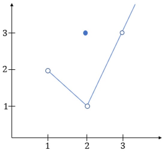
Consider

$$f:\mathbb{R}\to [0,+\infty ],\mathrm{d}\mathrm{e}\mathrm{f}\mathrm{i}\mathrm{n}\mathrm{e}\mathrm{d}\mathrm{a}\mathrm{s}f\left(x\right):=\left\{\begin{array}{cc}0,& ifx\in [0,1]\\ -x+3,& ifx\in (1,2)\\ 2,& ifx=2\\ x-1,& ifx\in (2,+\infty )\end{array}\right.$$

A simple calculation shows that

$${\ell }_{1}f=L_{1}f=[0,1],\mathrm{a}\mathrm{n}\mathrm{d}{\ell }_{1+\epsilon }f=[0,1]\cup (2-\epsilon ,2)\cup (2,2+\epsilon ),\epsilon \in (0,1)$$

implying that

$$\underset{\beta \to 1}{lim\; sup}{L}_{\beta }f=\bigcap _{\epsilon >0}\overline{{\ell }_{1+\epsilon }f}=[0,1]\cup \left\{2\right\}\mathrm{a}\mathrm{n}\mathrm{d}\underset{\beta \to 1}{lim\; inf}{L}_{\beta }f=\overline{{\ell }_{1}f}=[0,1].$$

Since for $\alpha \ne 1,{lim\; sup}_{\beta \to \alpha }{L}_{\beta }f=\overline{{\ell }_{\alpha }f}$, then necessarily $\mathcal{M}\left(f\right)={\mathcal{M}}_1\left(f\right)=\left\{2\right\}$. Note also that f has no minimum (see Figure 1).

Next, we define a weak level continuity of a level function.

Definition 7. 

For any $\alpha >0$, a function $f\in \mathcal{F}\left(X\right)$ is said to be weak α-level-continuous if ${\mathcal{M}}_{\alpha }\left(f\right)=\varnothing$. We say that f is weak level-continuous if it is weak α-level-continuous for all $\alpha >0$.

It is straightforward to see that $f\in \mathcal{F}\left(X\right)$ is weak level-continuous if

$$\forall \alpha >0,\underset{\beta \to \alpha }{lim}{L}_{\beta }f=\overline{L_{\alpha }f}.$$

3. Convergence by Level and by Epigraph

We introduce in this section the notions of level convergence and epigraph convergence and study the conditions that guarantee their equivalence.

Definition 8. 

Let ${\left(f_{\lambda }\right)}_{\lambda \in \Lambda }\subset \mathcal{F}\left(X\right)$ be a net. We say that $f_{\lambda }$ weak converges by a level (L-converges) to a function $f\in \mathcal{F}\left(X\right)$ (or simply $f_{\lambda }\stackrel{\mathrm{L}}{\to }f$) if

$$\forall \alpha >0,L_{\alpha }{f}_{\lambda }\to \overline{L_{\alpha }f}.$$

Analogously, a net ${\left(f_{\lambda }\right)}_{\lambda \in \Lambda }\subset \mathcal{F}\left(X\right)$ weak converges by an epigraph (E-converges) to a function $f\in \mathcal{F}\left(X\right)$ (or simply $f_{\lambda }\stackrel{\mathrm{E}}{\to }f$) when

$$E\left(f_{\lambda }\right)\to \overline{E\left(f\right)}.$$

We say that the function $f\in \mathcal{F}\left(X\right)$ is an L-limit of the net ${\left(f_{\lambda }\right)}_{\lambda \in \Lambda }$ if $f_{\lambda }\stackrel{L}{\to }f$ and an E-limit if $f_{\lambda }\stackrel{E}{\to }f$.

The next example shows that a net can be E-convergent but not L-convergent.

Example 3. 

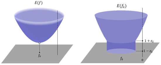
Let $(X,\Sigma ,\mu )$ be a measure space and $L^p(X,\nu )$ its associated Banach space. Let $f_0\in L^p(X,\nu )$ with $\parallel f_0{\parallel }_p>1$ and consider ${\left({\epsilon }_{\lambda }\right)}_{\lambda \in \Lambda }\subset (0,1)$ a decreasing net such that ${\epsilon }_{\lambda }\searrow 0$. Define

$$F_{\lambda }\left(f\right):=\left\{\begin{array}{cc}0,& iff=0\\ 1-{\epsilon }_{\lambda }& iff\in B(f_0,{\epsilon }_{\lambda })\\ \parallel f-f_0{\parallel }_p+1& otherwise\end{array}\right.\mathrm{and}F\left(f\right):=\left\{\begin{array}{cc}0,& iff=0\\ 2,& iff=f_0\\ \parallel f-f_0{\parallel }_p+1& otherwise\end{array}\right.,$$

where $B(f_0,{\epsilon }_{\lambda }):=\{f\in L^p(X,\nu );\parallel f-f_0{\parallel }_p<{\epsilon }_{\lambda }\}$ is the ${\epsilon }_{\lambda }$ ball in $L^p(X,\nu )$ centered at $f_0$. Since

$$B(f_0,{\epsilon }_{\lambda })\supset B(f_0,{\epsilon }_{\mu }),if\lambda \le \mu ,$$

we have that

$$\underset{\lambda }{lim}{L}_1{F}_{\lambda }=\bigcap _{\lambda }\overline{\left(B(f_0,{\epsilon }_{\lambda })\cup \left\{0\right\}\right)}=\{0,f_0\}.$$

On the other hand, $\overline{L_{1}F}=L_{1}f=\left\{0\right\}$, showing that $F_{\lambda }$ does not L-converge to F.

$$E\left(f\right)=\left\{0\right\}\times (0,+\infty )\cup \left\{f_0\right\}\times [2,+\infty )\cup \bigcup _{\alpha \in (1,+\infty )}\left(\overline{B(f_0,\alpha )}\times \left\{\alpha \right\}\right)$$

and so

$$\overline{E\left(f\right)}=\left\{0\right\}\times (0,+\infty )\cup \bigcup _{\alpha \in [1,+\infty )}\left(\overline{B(f_0,\alpha )}\times \left\{\alpha \right\}\right)$$

Also,

$$E\left(f_{\lambda }\right)=\left\{0\right\}\times (0,+\infty )\cup \overline{B(f_0,{\epsilon }_{\lambda })}\times [1-{\epsilon }_{\lambda },+\infty )\cup \bigcup _{\alpha \in [1+{\epsilon }_{\lambda },+\infty )}\left(\overline{B(f_0,\alpha )}\times \left\{\alpha \right\}\right),$$

implying that

$$\underset{\lambda }{lim}E\left(f_{\lambda }\right)=\left\{0\right\}\times (0,+\infty )\cup \bigcup _{\alpha \in [1,+\infty )}\left(\overline{B(f_0,\alpha )}\times \left\{\alpha \right\}\right)=\overline{E\left(f\right)},$$

and, hence, $f_{\lambda }\stackrel{E}{\to }f$ (see Figure 2).

Remark 2. 

A simple calculation shows us that

$$L_{\alpha }{F}_{\lambda }=\left\{\begin{array}{cc}\left\{0\right\},& if\alpha \in (0,1-{\epsilon }_{\lambda })\\ \overline{B(f_0,{\epsilon }_{\lambda })}\cup \left\{0\right\}& if\alpha \in [1-{\epsilon }_{\lambda },1]\\ \overline{B(0,\alpha )}\cup \left\{0\right\},& if\alpha >1\}\end{array}\right.$$

implying that the functions $F_{\lambda }$ in Example 3 are also lower semicontinuous.

The subsequent lemma relates the limits of epigraphs and level sets, a relation that will be essential in the proof of our main theorem.

Lemma 1. 

For all $\alpha >0$, the following holds:

1. 

$x\in {lim\; sup}_{\lambda }{L}_{\alpha }{f}_{\lambda }\Rightarrow (x,\alpha )\in {lim\; sup}_{\lambda }E\left(f_{\lambda }\right);$

2. 

$x\in {lim\; inf}_{\lambda }{L}_{\alpha }{f}_{\lambda }\Rightarrow (x,\alpha )\in {lim\; inf}_{\lambda }E\left(f_{\lambda }\right);$

3. 

$(x,\alpha )\in {lim\; sup}_{\lambda }E\left(f_{\lambda }\right)\Rightarrow \forall \epsilon >0,x\in {lim\; sup}_{\lambda }{L}_{\alpha +\epsilon }{f}_{\lambda };$

4. 

$(x,\alpha )\in {lim\; inf}_{\lambda }E\left(f_{\lambda }\right)\Rightarrow \forall \epsilon >0,x\in {lim\; inf}_{\lambda }{L}_{\alpha +\epsilon }{f}_{\lambda }.$

Proof. 

Since the items 1. and 3. are analogous to 2. and 4., respectively, we will only show 1. and 4.

1. Let $x\in {lim\; sup}_{\lambda }{L}_{\alpha }{f}_{\lambda }$. By definition, there exists a subnet ${\lambda }_{\mu }\to +\infty$ and $x_{{\lambda }_{\mu }}\in L_{\alpha }{f}_{{\lambda }_{\mu }}$ with $x_{{\lambda }_{\mu }}\to x$. Consequently,

$$(x_{{\lambda }_{\mu }},\alpha )\in E\left(f_{{\lambda }_{\mu }}\right)\mathrm{a}\mathrm{n}\mathrm{d}(x_{{\lambda }_{\mu }},\alpha )\to (x,\alpha )\Rightarrow (x,\alpha )\in \underset{\lambda }{lim\; sup}E\left(f_{\lambda }\right).$$

4. Let $(x,\alpha )\in {lim\; inf}_{\lambda }E\left(f_{\lambda }\right)$ and $\epsilon >0$. For any ${\lambda }_{\mu }\to +\infty$,

$$\exists (x_{{\lambda }_{\mu }},{\alpha }_{{\lambda }_{\mu }})\in E\left(f_{{\lambda }_{\mu }}\right)\mathrm{s}\mathrm{u}\mathrm{c}\mathrm{h}\mathrm{t}\mathrm{h}\mathrm{a}\mathrm{t}(x_{{\lambda }_{\mu }},{\alpha }_{{\lambda }_{\mu }})\to (x,\alpha ).$$

In particular, ${\alpha }_{{\lambda }_{\mu }}\to \alpha$ implies the existence of ${\mu }_0\in \Lambda$ such that ${\alpha }_{{\lambda }_{\mu }}<\alpha +\epsilon$ if $\mu \ge {\mu }_0$ and, hence,

$$(x_{{\lambda }_{\mu }},{\alpha }_{{\lambda }_{\mu }})\in E\left(f_{{\lambda }_{\mu }}\right)\Rightarrow x_{{\lambda }_{\mu }}\in L_{{\alpha }_{{\lambda }_{\mu }}}f\subset L_{\alpha +\epsilon }{f}_{{\lambda }_{\mu }},if\mu \ge {\mu }_0,$$

showing that $x\in {lim\; inf}_{\lambda }{L}_{\alpha +\epsilon }f$ and finishing the proof. □

Now, we can state and prove our main result concerning the level and the epigraph convergence.

Theorem 1. 

Let ${\left(f_{\lambda }\right)}_{\lambda \in \Lambda }\subset \mathcal{F}\left(X\right)$ be a net and $f\in \mathcal{F}\left(X\right)$. Then,

$$f_{\lambda }\stackrel{\mathrm{L}}{\to }f\Rightarrow f_{\lambda }\stackrel{\mathrm{E}}{\to }f.$$

Reciprocally, if f is level-continuous, then

$$f_{\lambda }\stackrel{\mathrm{E}}{\to }f\Rightarrow f_{\lambda }\stackrel{\mathrm{L}}{\to }f.$$

Proof. 

We have to show that

$$f_{\lambda }\stackrel{\mathrm{L}}{\to }f\Rightarrow \underset{\lambda }{lim\; sup}E\left(f_{\lambda }\right)\subset \overline{E\left(f\right)}\subset \underset{\lambda }{lim\; inf}E\left(f_{\lambda }\right).$$

However, by Lemma 1,

$$(x,\alpha )\in \underset{\lambda }{lim\; sup}E\left(f_{\lambda }\right)\Rightarrow x\in \underset{\lambda }{lim\; sup}{L}_{\alpha +\epsilon }{f}_{\lambda },\forall \epsilon >0,$$

and, hence,

$$f_{\lambda }\stackrel{L}{\to }f\Rightarrow x\in \overline{L_{\alpha +\epsilon }f}\subset \overline{{\ell }_{\alpha +2\epsilon }f},\forall \epsilon >0.$$

By Propositions 2 and 3, we conclude that

$$x\in \bigcap _{\epsilon >0}\overline{l_{\alpha +2\epsilon }f}=\underset{\beta \to \alpha }{lim\; sup}{L}_{\beta }f\Rightarrow (x,\alpha )\in \left(\underset{\beta \to \alpha }{lim\; sup}{L}_{\beta }f\times \left\{\alpha \right\}\right)\subset \overline{E\left(f\right)},$$

thus ${lim\; sup}_{\lambda }E\left(f_{\lambda }\right)\subset \overline{E\left(f\right)}$.

Let us consider now $(x,\alpha )\in E\left(f\right)$. Then, $x\in L_{\alpha }f$ and the assumption $f_{\lambda }\stackrel{L}{\to }f$ together with Lemma 1 imply

$$x\in L_{\alpha }f\subset \overline{L_{\alpha }f}=\underset{\lambda }{lim\; inf}{L}_{\alpha }{f}_{\lambda }\Rightarrow (x,\alpha )\in \underset{\lambda }{lim\; inf}E\left(f_{\lambda }\right).$$

Therefore, $E\left(f\right)\subset {lim\; inf}_{\lambda }E\left(f_{\lambda }\right)$, so $\overline{E\left(f\right)}\subset {lim\; inf}_{\lambda }E\left(f_{\lambda }\right)$ and then $f_{\lambda }\stackrel{E}{\to }f$.

Let us now assume that $f_{\lambda }\stackrel{E}{\to }f$ with f is level-continuous. By definition,

$$f_{\lambda }\stackrel{L}{\to }f\iff \forall \alpha >0,\underset{\lambda }{lim\; sup}{L}_{\alpha }{f}_{\lambda }\subset \overline{L_{\alpha }f}\subset \underset{\lambda }{lim\; inf}{L}_{\alpha }{f}_{\lambda }.$$

Let $\alpha >0$ and $x\in {lim\; sup}_{\lambda }{L}_{\alpha }{f}_{\lambda }$. Since we are assuming that $f_{\lambda }\stackrel{E}{\to }f$, we have by Lemma 1 and Proposition 3 that

$$(x,\alpha )\in \underset{\lambda }{lim\; sup}E\left(f_{\lambda }\right)=\overline{E\left(f\right)}=\bigcup _{\alpha >0}\left(\underset{\beta \to \alpha }{lim\; sup}{L}_{\beta }f\times \left\{\alpha \right\}\right).$$

Therefore, $x\in {lim\; sup}_{\beta \to \alpha }{L}_{\beta }f$ and, since we are assuming that f is level-continuous,

$$x\in \underset{\beta \to \alpha }{lim\; sup}{L}_{\beta }f=\overline{L_{\alpha }f},\mathrm{which}\mathrm{implies}\underset{\lambda }{lim\; sup}{L}_{\alpha }{f}_{\lambda }\subset \overline{L_{\alpha }f}.$$

Consider now $x\in {\ell }_{\alpha }f$ and define ${\alpha }_0:=f\left(x\right)<\alpha$, then $(x,{\alpha }_0)\in E\left(f\right)$. Since we are assuming $f_{\lambda }\stackrel{E}{\to }f$, we obtain from Lemma 1 that

$$(x,{\alpha }_0)\in E\left(f\right)\subset \underset{\lambda }{lim\; inf}E\left(f_{\lambda }\right)\Rightarrow \forall \epsilon >0,x\in \underset{\lambda }{lim\; inf}{L}_{{\alpha }_0+\epsilon }f.$$

Hence, for $\epsilon >0$ small enough, we obtain

$$L_{{\alpha }_0+\epsilon }{f}_{\lambda }\subset L_{\alpha }{f}_{\lambda }\Rightarrow x\in \underset{\lambda }{lim\; inf}{L}_{{\alpha }_0+\epsilon }f\subset \underset{\lambda }{lim\; inf}{L}_{\alpha }{f}_{\lambda }\Rightarrow {\ell }_{\alpha }f\subset \underset{\lambda }{lim\; inf}{L}_{\alpha }{f}_{\lambda }.$$

On the other hand, we are assuming that f is level-continuous, in particular, $\overline{L_{\alpha }f}=\overline{{\ell }_{\alpha }f}$ and consequently

$$\overline{L_{\alpha }f}=\overline{{\ell }_{\alpha }f}\subset \underset{\lambda }{lim\; inf}{L}_{\alpha }{f}_{\lambda }$$

which implies that $f_{\lambda }\stackrel{L}{\to }f$ ending the proof. □

The next step is to define monotone increasing nets.

Definition 9. 

We say that a net ${\left(f_{\lambda }\right)}_{\lambda \in \Lambda }\subset \mathcal{F}\left(X\right)$ is monotone increasing if the net ${\left(E\left(f_{\lambda }\right)\right)}_{\lambda \in \Lambda }$ is monotone increasing.

The next lemma states the main properties of monotone increasing nets.

Lemma 2. 

For any net ${\left(f_{\lambda }\right)}_{\lambda \in \Lambda }\subset \mathcal{F}\left(X\right)$, the following holds:

1. 

${\left(f_{\lambda }\right)}_{\lambda \in \Lambda }$ is monotone increasing if ${\left(L_{\alpha }{f}_{\lambda }\right)}_{\lambda \in \Lambda }$ is monotone increasing for all $\alpha >0$.

2. 

If ${\left(f_{\lambda }\right)}_{\lambda \in \Lambda }$ is monotone increasing, then, for all $x\in X$, the net ${\left(f_{\lambda }\left(x\right)\right)}_{\lambda \in \Lambda }$ is monotone decreasing.

Proof. 

1. In this case,

$$\forall \alpha >0,x\in L_{\alpha }{f}_{\lambda }\Rightarrow (x,\alpha )\in E\left(f_{\lambda }\right)\subset E\left(f_{\mu }\right)\Rightarrow x\in L_{\alpha }{f}_{\mu }.$$

Reciprocally, if $\forall \alpha >0,L_{\alpha }{f}_{\lambda }\subset L_{\alpha }{f}_{\mu }$, then

$$(x,\alpha )\in E\left(f_{\lambda }\right)\Rightarrow x\in L_{\alpha }{f}_{\lambda }\subset L_{\alpha }{f}_{\mu }\Rightarrow (x,\alpha )\in E\left(f_{\mu }\right).$$

2. Let $x\in X$ and $\lambda \le \mu$. Then,

$$(x,f_{\lambda }\left(x\right))\in E\left(f_{\lambda }\right)\subset E\left(f_{\mu }\right)\Rightarrow f_{\mu }\left(x\right)\le f_{\lambda }\left(x\right)\Rightarrow {\left(f_{\lambda }\left(x\right)\right)}_{\lambda \in \Lambda }\mathrm{i}\mathrm{s}\mathrm{d}\mathrm{e}\mathrm{c}\mathrm{r}\mathrm{e}\mathrm{a}\mathrm{s}\mathrm{i}\mathrm{n}\mathrm{g}.$$

□

The next theorem shows that monotone increasing nets are E-convergent.

Theorem 2. 

Any monotone increasing net has an E-limit in $\mathcal{F}\left(X\right)$.

Proof. 

By Lemma 2, we have that ${\left(f_{\lambda }\left(x\right)\right)}_{\lambda \in \Lambda }$ is a monotone-decreasing sequence. By the Monotone Converge Theorem for real sequences, we obtain that ${\left(f_{\lambda }\left(x\right)\right)}_{\lambda \in \Lambda }$ converges to $f\left(x\right):={inf}_{\lambda \in \Lambda }{f}_{\lambda }\left(x\right)$. Moreover,

$$f_{\lambda }\in \mathcal{F}\left(X\right),\lambda \in \Lambda \Rightarrow f\in \mathcal{F}\left(X\right).$$

Also,

$${\left(f_{\lambda }\right)}_{\lambda \in \Lambda }\mathrm{i}\mathrm{n}\mathrm{c}\mathrm{r}\mathrm{e}\mathrm{a}\mathrm{s}\mathrm{i}\mathrm{n}\mathrm{g}\Rightarrow \underset{\lambda }{lim}E\left(f_{\lambda }\right)=\overline{\bigcup _{\lambda \in \Lambda }E\left(f_{\lambda }\right)}\mathrm{a}\mathrm{n}\mathrm{d},\mathrm{h}\mathrm{e}\mathrm{n}\mathrm{c}\mathrm{e},f_{\lambda }\stackrel{E}{\to }f\iff \overline{E\left(f\right)}=\overline{\bigcup _{\lambda \in \Lambda }E\left(f_{\lambda }\right)}.$$

If $(x,\alpha )\in E\left(f_{\lambda }\right)$ for some $\lambda \in \Lambda$ then $f\left(x\right)\le f_{\lambda }\left(x\right)\le \alpha$ and hence

$$\overline{\bigcup _{\lambda \in \Lambda }E\left(f_{\lambda }\right)}\subset \overline{E\left(f\right)}.$$

On the other hand, let $(x,\alpha )\in E\left(f\right)$. For any $U\in {\mathcal{V}}_{(x,\alpha )}$, there exists ${\alpha }_U>\alpha$ such that $(x,{\alpha }_U)\in U$. Hence,

$$f\left(x\right)\le \alpha <{\alpha }_U\Rightarrow \exists \lambda \in \Lambda ;f_{\lambda }\left(x\right)<{\alpha }_U\Rightarrow (x,{\alpha }_U)\in E\left(f_{\lambda }\right)\subset \bigcup _{\lambda \in \Lambda }E\left(f_{\lambda }\right).$$

Hence, the net ${\left((x,{\alpha }_U)\right)}_{U\in {\mathcal{V}}_{(x,\alpha )}}$ is contained in ${\bigcup }_{\lambda \in \Lambda }E\left(f_{\lambda }\right)$ and $(x,{\alpha }_U)\to (x,\alpha )$, implying that

$$E\left(f\right)\subset \overline{\bigcup _{\lambda \in \Lambda }E\left(f_{\lambda }\right)},$$

and concluding the proof. □

Remark 3. 

An analogous definition can be given for monotone-decreasing nets. However, there is no guarantee that a monotone-decreasing net admits a limit in $\mathcal{F}\left(X\right)$.

4. Robust Functions and Topological Groups

This section is devoted to the study of robust functions on topological groups. Such functions arise naturally in optimization problems, and a thorough understanding of them is, therefore, highly desirable (see, for instance, [6,7]). Our aim is to show that any level function on a topological group can be realized as the limit of robust functions with respect to both level convergence and epigraph convergence.

Definition 10. 

A subset $A\subseteq X$ is said to be robust if $\overline{A}=\overline{intA}$.

We define the class of L-robust functions of $\mathcal{F}\left(X\right)$ as

$${\mathcal{R}}_L\left(X\right):=\{f\in \mathcal{F}\left(X\right);{\ell }_{\alpha }f\mathrm{i}\mathrm{s}\mathrm{r}\mathrm{o}\mathrm{b}\mathrm{u}\mathrm{s}\mathrm{t}\forall \alpha >0\}.$$

and the class of E-robust functions of $\mathcal{F}\left(X\right)$ as

$${\mathcal{R}}_E\left(X\right):=\{f\in \mathcal{F}\left(X\right);e\left(f\right)\mathrm{i}\mathrm{s}\mathrm{r}\mathrm{o}\mathrm{b}\mathrm{u}\mathrm{s}\mathrm{t}\}.$$

By Proposition 3, it holds that ${\mathcal{R}}_L\left(X\right)\subset {\mathcal{R}}_E\left(X\right)$.

4.1. Topological Groups

Let G be a topological Hausdorff group. For any $x\in G$, the right translation by x is the map

$$R_x:G\to G,y\in G\mapsto yx\in G.$$

It is a standard fact that $R_x$ is a homeomorphism of G with the inverse given by $R_{x^{-1}}$, where $x^{-1}$ is the unique element in G such that $x{x}^{-1}=x^{-1}x=e$, with $e\in G$ the identity element.

For any given nonempty subsets $A,B\subseteq G$, we define the set

$$AB=\{ab/a\in A,b\in B\}.$$

Proposition 4. 

Let A and B be two nonempty subsets of G. The following holds:

1. 

If A is open, then $AB$ is open;

2. 

If $intA\ne \varnothing$, then $\left(intA\right)B\subseteq intAB$;

3. 

If A is robust, then $AB$ is robust.

Proof. 

The proofs of items 1 and 2 are straightforward. For item 3, we only have to show that $\overline{AB}\subset \overline{intAB}$ since the opposite inclusion always holds. Let then $x\in \overline{AB}$ and consider a neighborhood U of x. By definition,

$$U\cap AB\ne \varnothing \Rightarrow ab\in U,\mathrm{f}\mathrm{o}\mathrm{r}\mathrm{s}\mathrm{o}\mathrm{m}\mathrm{e}a\in A,b\in B.$$

In particular, $a\in U{b}^{-1}$ and, hence, $U{b}^{-1}$ is a neighborhood of a since translations are homeomorphisms. By the assumption that A is robust, we have that

$$\exists a^{\prime }\in intA\mathrm{with}{a}^{\prime }\in U{b}^{-1}\Rightarrow a^{\prime }b\in U\Rightarrow \left(intA\right)B\cap U\ne \varnothing ,$$

and by item 2, we conclude that $intAB\cap U\ne \varnothing$ and, hence, $x\in \overline{intAB}$ concluding the proof. □

4.2. L-Robust Functions on Topological Groups

In this section, we show that on topological groups, any function in $\mathcal{F}\left(G\right)$ is the L-limit of some net ${\left(f_{\lambda }\right)}_{\lambda \in \Lambda }\in {\mathcal{R}}_L\left(G\right)$.

Let $f,g\in \mathcal{F}\left(G\right)$. The L-convolution of f and g is the function $f{*}_{L}g\in \mathcal{F}\left(G\right)$ given by

$$f{*}_{L}g\left(x\right):=\underset{y\in G}{inf}\{max\{f\left(x{y}^{-1}\right),g\left(y\right)\}\}$$

Lemma 3. 

For all $f,g\in \mathcal{F}\left(G\right)$ and $\alpha >0$, it holds that

1. 

${\ell }_{\alpha }\left(f{*}_{L}g\right)={\ell }_{\alpha }f{\ell }_{\alpha }g$;

2. 

$L_{\alpha }f{L}_{\alpha }g\subset L_{\alpha }\left(f{*}_{L}g\right);$

3. 

If there exists ${\epsilon }_0>0$ such that ${\ell }_{\alpha +\epsilon }g$ is open for all $\epsilon \in (0,{\epsilon }_0)$, then

$$L_{\alpha }\left(f{*}_{L}g\right)\setminus {\mathcal{M}}_{\alpha }\left(f\right)\subset \bigcap _{\epsilon \in (0,{\epsilon }_0)}\left({\ell }_{\alpha }f{\ell }_{\alpha +\epsilon }g\right).$$

Proof. 

1. Let $x\in {\ell }_{\alpha }(f*g)$. Then,

$$f*g\left(x\right)<\alpha \Rightarrow \underset{y\in G}{inf}\{max\{f\left(x{y}^{-1}\right),g\left(y\right)\}\}<\alpha \Rightarrow \exists y\in G;max\{f\left(x{y}^{-1}\right),g\left(y\right)\}<\alpha$$

$$\Rightarrow \exists y\in G;f\left(x{y}^{-1}\right)>\alpha \mathrm{and}g\left(y\right)<\alpha \Rightarrow x{y}^{-1}\in {\ell }_{\alpha }f\mathrm{and}y\in {\ell }_{\alpha }g\Rightarrow x=\left(x{y}^{-1}\right)y\in {\ell }_{\alpha }f{\ell }_{\alpha },g$$

which proves that ${\ell }_{\alpha }\left(f{*}_{L}g\right)\subset {\ell }_{\alpha }f{\ell }_{\alpha }g$.

Reciprocally, if $a\in {\ell }_{\alpha }f$ and $b\in {\ell }_{\alpha }g$, then

$$max\left\{f\left(\left(ab\right)b^{-1}\right),g\left(b\right)\right\}<\alpha \Rightarrow f*g\left(ab\right)=\underset{y\in G}{inf}\left\{max\left\{f\left(\left(ab\right)y^{-1}\right),g\left(y\right)\right\}\right\}<\alpha ,$$

showing that ${\ell }_{\alpha }f{\ell }_{\alpha }g\subset {\ell }_{\alpha }(f*g)$ and so ${\ell }_{\alpha }\left(f{*}_{L}g\right)={\ell }_{\alpha }f{\ell }_{\alpha }g$.

2. It follows analogously from the inclusion ${\ell }_{\alpha }f{\ell }_{\alpha }g\subset {\ell }_{\alpha }\left(f{*}_{L}g\right)$.

3. By definition, for any $\epsilon >0$, there exists $y\in G$ such that

$$f{*}_{L}g\left(x\right)+\epsilon >max\{f\left(x{y}^{-1}\right),g\left(y\right)\}\Rightarrow f\left(x{y}^{-1}\right)<\alpha +\epsilon \mathrm{and}g\left(y\right)<\alpha +\epsilon$$

$$\Rightarrow x{y}^{-1}\in {\ell }_{\alpha +\epsilon }f\mathrm{and}y\in {\ell }_{\alpha +\epsilon }g\iff x{\left({\ell }_{\alpha +\epsilon }g\right)}^{-1}\cap {\ell }_{\alpha +\epsilon }f\ne \varnothing .$$

In particular, we obtain that

$$x{\left({\ell }_{\alpha +\epsilon }g\right)}^{-1}\cap {\ell }_{\alpha +\delta }f\ne \varnothing ,\forall \epsilon \in (0,{\epsilon }_0)\mathrm{and}\delta >0.$$

However, by hypothesis, $x{\left({\ell }_{\alpha +\epsilon }g\right)}^{-1}\in {\mathcal{V}}_x$ for any $\epsilon \in (0,{\epsilon }_0)$ and, hence,

$$x\in L_{\alpha }\left(f{*}_{L}g\right)\setminus {\mathcal{M}}_{\alpha }\left(f\right)\Rightarrow x{\left({\ell }_{\alpha +\epsilon }g\right)}^{-1}\cap {\ell }_{\alpha }f\ne \varnothing ,\forall \epsilon \in (0,{\epsilon }_0).$$

Therefore,

$$x\in {\ell }_{\alpha }{\ell }_{\alpha +\epsilon }g,\forall \epsilon \in (0,{\epsilon }_0)\Rightarrow x\in \bigcap _{\epsilon \in (0,{\epsilon }_0)}\left({\ell }_{\alpha }f{\ell }_{\alpha +\epsilon }g\right),$$

which ends the proof. □

Next, we prove that all functions in $\mathcal{F}\left(G\right)$ are L-limits of robust functions.

Theorem 3. 

For any $f\in \mathcal{F}\left(G\right)$, there exists a net ${\left(f_{\lambda }\right)}_{\lambda \in \Lambda }\subset {\mathcal{R}}_L\left(G\right)$ such that

$$f_{\lambda }\stackrel{L}{\to }f.$$

Proof. 

For any $U\in {\mathcal{V}}_e$, let us consider the indicator function of U given by

$$g_U\left(x\right):=\left\{\begin{array}{cc}0,\hfill & ifx\in U\hfill \\ +\infty \hfill & ifx\notin U\hfill \end{array}\right.\mathrm{and}\mathrm{define}{f}_U\left(x\right):=\left\{\begin{array}{cc}f{*}_L{g}_U\left(x\right),\hfill & ifx\notin \mathcal{M}\left(f\right)\hfill \\ f\left(x\right),\hfill & ifx\in \mathcal{M}\left(f\right)\hfill \end{array}\right..$$

For all $\alpha >0$, it holds that

$$x\in {\ell }_{\alpha }{f}_U\iff f{*}_{L}g\left(x\right)<\alpha orf\left(x\right)<\alpha \iff x\in {\ell }_{\alpha }\left(f{*}_L{g}_U\right)orx\in {\ell }_{\alpha }f.$$

However, by definition ${\ell }_{\alpha }{g}_U=U$, which by Lemma 3 implies that ${\ell }_{\alpha }\left(f{*}_{L}g\right)={\ell }_{\alpha }fU$, and, since $U\in {\mathcal{V}}_e$, we obtain that ${\ell }_{\alpha }f\subset {\ell }_{\alpha }fU.$ By Proposition 4, it follows that

$${\ell }_{\alpha }{f}_U={\ell }_{\alpha }(f*g_U)={\ell }_{\alpha }fU\Rightarrow f_U\in {\mathcal{R}}_L\left(G\right);$$

thus, we only have to show that ${\left(f_U\right)}_{U\in {\mathcal{V}}_e}$L-converges to f, that is,

$$\underset{U}{lim\; sup}{L}_{\alpha }{f}_U\subset L_{\alpha }f\subset \underset{U}{lim\; inf}{L}_{\alpha }{f}_U,\forall \alpha >0.$$

Let us first note that if $x\in \mathcal{M}\left(f\right)$, by definition, $f*g_U\left(x\right)=f\left(x\right)$ for all $U\in {\mathcal{V}}_e$; hence, we only have to show the previous relation for $x\notin \mathcal{M}\left(f\right)$.

Consider $x\in {lim\; sup}_U{L}_{\alpha }{f}_U\setminus {\mathcal{M}}_{\alpha }\left(f\right)$. We have

$$\exists \left\{U_{\lambda }\right\}\subset {\mathcal{V}}_e\mathrm{and}{x}_{\lambda }\in L_{\alpha }{f}_{U_{\lambda }}\mathrm{such}\mathrm{that}\bigcap _{\lambda }{U}_{\lambda }=\left\{e\right\}\mathrm{and}{x}_{\lambda }\to x.$$

If there exists a subnet $x_{{\lambda }_{\mu }}\in {\mathcal{M}}_G\left(f\right)$ such that $x_{{\lambda }_{\mu }}\to x$, then

$$f\left(x_{{\lambda }_{\mu }}\right)=f_{U_{\lambda }}\left(x_{{\lambda }_{\mu }}\right)\le \alpha \Rightarrow x_{{\lambda }_{\mu }}\in L_{\alpha }f\Rightarrow x\in \overline{L_{\alpha }f}.$$

Therefore, we can assume w.l.o.g. that $x_{\lambda }\in L_{\alpha }{f}_{U_{\lambda }}\setminus {\mathcal{M}}_{\alpha }\left(f\right)$ for all $\lambda$. In this case, the fact that ${\ell }_{\alpha +\epsilon }{g}_{U_{\lambda }}=U_{\lambda }$ for all $\epsilon >0$ implies by item 3 in Proposition 3 that

$$L_{\alpha }\left(f{*}_L{g}_{U_{\lambda }}\right)\setminus {\mathcal{M}}_G\left(f\right)\subset \bigcap _{\epsilon >0}\left({\ell }_{\alpha }f{\ell }_{\alpha +\epsilon }{g}_{U_{\lambda }}\right)={\ell }_{\alpha }f{U}_{\lambda }.$$

Therefore,

$$\forall \lambda ,\exists a_{\lambda }\in {\ell }_{\alpha }f\mathrm{and}{b}_{\lambda }\in U_{\lambda };\mathrm{such}\mathrm{that}{x}_{\lambda }=a_{\lambda }{b}_{\lambda }.$$

However, $b_{\lambda }\in U_{\lambda }$ implies that $b_{\lambda }\to e$ and, hence, $a_{\lambda }=x{b}_{\lambda }^{-1}\to x$. Since $a_{\lambda }\in {\ell }_{\alpha }f$ we obtain that $x\in \overline{{\ell }_{\alpha }f}\subset \overline{L_{\alpha }f}$ implying that

$$\underset{U}{lim\; sup}{L}_{\alpha }{f}_U\subset \overline{L_{\alpha }f}.$$

Consider now $x\in L_{\alpha }f\setminus {\mathcal{M}}_{\alpha }\left(f\right)$ and a family $\left\{U_{\lambda }\right\}\subset {\mathcal{V}}_e$ such that ${\bigcap }_{\lambda }{U}_{\lambda }=\left\{e\right\}$. By choosing $b_{\lambda }\in U_{\lambda }$ we have that $x{b}_{\lambda }\to x$ and, by item 2 in Proposition 3 that

$$x{b}_{\lambda }\in L_{\alpha }f{U}_{\lambda }=L_{\alpha }f{L}_{\alpha }{g}_{U_{\lambda }}\subset L\left(f{*}_L{g}_{U_{\lambda }}\right)$$

implying that $x\in {lim\; inf}_U{L}_{\alpha }(f*g_U)$ and hence $f_U\stackrel{L}{\to }f$. □

4.3. E-Robust Functions on Topological Groups

In this section, we show that on topological groups, it is also true that any function in $\mathcal{F}\left(G\right)$ is the E-limit of some net ${\left(f_{\lambda }\right)}_{\lambda \in \Lambda }\in {\mathcal{R}}_E\left(G\right)$.

Let us consider $G\times \mathbb{R}$ as a topological group, with the product given by

$$(x_1,{\alpha }_1)(x_2,{\alpha }_2):=(x_1·x_2,{\alpha }_1+{\alpha }_2).$$

Let $f,g\in \mathcal{F}\left(G\right)$. The E-convolution of f and g is the function $f{*}_{E}g\in \mathcal{F}\left(G\right)$ given by

$$f{*}_{E}g\left(x\right):=\underset{y\in G}{inf}\{f\left(x{y}^{-1}\right)+g\left(y\right)\}.$$

Lemma 4. 

For all $f,g\in \mathcal{F}\left(G\right)$ and $\alpha >0$, it holds that

1. 

$e\left(f{*}_{E}g\right)=e\left(f\right)e\left(g\right)$;

2. 

$E\left(f\right)E\left(g\right)\subset E\left(f{*}_{E}g\right)\subset \overline{E\left(f\right)E\left(g\right)};$

3. 

$e\left(f\right)$ and $E\left(f\right)$ are invariant for translations by elements in $\left\{e\right\}\times \mathbb{R}$.

Proof. 

1. Let $(x,\alpha )\in e(f*g)$. In particular, if $\epsilon >0$ is such that $f{*}_{E}g\left(x\right)<\alpha -\epsilon$, there exists $y\in G$ and such that

$$f\left(x{y}^{-1}\right)+g\left(y\right)+\epsilon <\alpha .$$

Then, $(x_1,{\alpha }_1)=(x{y}^{-1},f\left(x{y}^{-1}\right)+\epsilon )$ and $(x_2,{\alpha }_2)=(y,\alpha -f\left(x{y}^{-1}\right)-\epsilon )$ are such that

$$(x_1,{\alpha }_1)\in e\left(g\right)\mathrm{and}(x_2,{\alpha }_2)\in e\left(g\right)$$

and

$$(x_1,{\alpha }_1)(x_2,{\alpha }_2)=(x_1{x}_2,{\alpha }_1+{\alpha }_2)=(x,\alpha )\Rightarrow e\left(f{*}_{E}g\right)\subset e\left(f\right)e\left(g\right).$$

Reciprocally, if $(x_1,{\alpha }_1)\in e\left(f\right)$ and $(x_2,{\alpha }_2)\in e\left(g\right)$, then $f\left(x_1\right)<{\alpha }_1$ and $g\left(x_2\right)<{\alpha }_2$ give us

$${\alpha }_1+{\alpha }_2>f\left(x_1\right)+g\left(x_2\right)=f\left(\left(x_1{x}_2\right)x_2^{-1}\right)+g\left(x_2\right)\ge \underset{y\in G}{inf}\{f\left(\left(x_1{x}_2\right)y^{-1}\right)+g\left(y\right)\}=\left(f{*}_{E}g\right)\left(x_1{x}_2\right)$$

implying that $(x_1,{\alpha }_1)(x_2,{\alpha }_2)=(x_1{x}_2,{\alpha }_1+{\alpha }_2)\in e(f*g)$ and, hence,

$$e\left(f\right)e\left(g\right)\subset e\left(f{*}_{E}g\right).$$

2. The inclusion $E\left(f\right)E\left(g\right)\subset E\left(f{*}_{E}g\right)$ is analogous to the inclusion $e\left(f\right)e\left(g\right)\subset e\left(f{*}_{E}g\right)$. Consider then $(x,\alpha )\in E(f*g)$. By definition, for any $\epsilon >0$, there exists $y\in G$ such that

$$f\left(x{y}^{-1}\right)+g\left(y\right)<\alpha +\epsilon .$$

By defining $(x_1,{\alpha }_1)=(x{y}^{-1},f\left(x{y}^{-1}\right))$ and $(x_2,{\alpha }_2)=(y,\alpha +\epsilon -f\left(x{y}^{-1}\right))$, we obtain that

$$(x_1,{\alpha }_1)\in E\left(f\right)\mathrm{and}(x_2,{\alpha }_2)\in E\left(g\right);$$

furthermore,

$$(x_1,{\alpha }_1)(x_2,{\alpha }_2)=(x_1{x}_2,{\alpha }_1+{\alpha }_2)=(x,\alpha +\epsilon )\Rightarrow (x,\alpha +\epsilon )\in E\left(f\right)E\left(g\right),$$

implying that

$$(x,\alpha )\in \overline{E\left(f\right)E\left(g\right)}\mathrm{and}\mathrm{hence}E(f*g)\subset \overline{E\left(f\right)E\left(g\right)},$$

which finishes the proof. □

The next result shows that any function in $f\in \mathcal{F}\left(G\right)$ is the E-limit of a net in ${\mathcal{R}}_E\left(G\right)$.

Theorem 4. 

For any $f\in \mathcal{F}\left(G\right)$, there exists a net ${\left(f_{\lambda }\right)}_{\lambda \in \Lambda }\subset {\mathcal{R}}_E\left(G\right)$ such that

$$f_{\lambda }\stackrel{E}{\to }f.$$

Proof. 

For any $U\in {\mathcal{V}}_e$, let us consider indicator function of U given by

$$g_U\left(x\right):=\left\{\begin{array}{cc}0,\hfill & ifx\in U\hfill \\ +\infty \hfill & ifx\notin U\hfill \end{array}\right.$$

Then, $e\left(g_U\right)=U\times (0,+\infty )$ and, hence, $g_U\in \mathcal{R}\left(G\right)$. Moreover, by Lemma 4, it holds that

$$e(f*g_U)=e\left(f\right)e\left(g_U\right)=e\left(f\right)(U\times {\mathbb{R}}^{+}),$$

and so Proposition 4 assures that $e(f*g_U)$ is open and, in particular, robust. We claim that $f_U\stackrel{E}{\to }f$, or equivalently,

$$\underset{U}{lim\; sup}E\left(f_U\right)\subset \overline{E\left(f\right)}\subset \underset{U}{lim\; inf}E\left(f_U\right).$$

Let us consider $(x,\alpha )\in {lim\; sup}_{U}E\left(f_U\right)$. By definition,

$$\exists \left\{U_{\lambda }\right\}\subset {\mathcal{V}}_e\mathrm{and}(x_{\lambda },{\alpha }_{\lambda })\in E\left(f_{U_{\lambda }}\right)\mathrm{such}\mathrm{that}\bigcap _{\lambda }{U}_{\lambda }=\left\{e\right\}\mathrm{and}(x_{\lambda },{\alpha }_{\lambda })\to (x,\alpha ).$$

Moreover, from Lemma 4, it holds that $E\left(f_U\right)\subset \overline{E\left(f\right)E\left(g_U\right)}$; we can assume w.l.o.g. that

$$(x_{\lambda },{\alpha }_{\lambda })\in E\left(f\right)E\left(g_{U_{\lambda }}\right),$$

so we can write

$$(x_{\lambda },{\alpha }_{\lambda })=(a_{\lambda },{\gamma }_{\lambda })(b_{\lambda },{\beta }_{\lambda }),\mathrm{with}(a_{\lambda },{\gamma }_{\lambda })\in E\left(f\right),\mathrm{and}(b_{\lambda },{\beta }_{\lambda })\in E\left(g_{U_{\lambda }}\right).$$

However,

$$(b_{\lambda },{\beta }_{\lambda })\in e\left(g_{U_{\lambda }}\right)=U_{\lambda }\times {\mathbb{R}}^{+}\Rightarrow b_{\lambda }\to e\Rightarrow a_{\lambda }=x_{\lambda }{b}_{\lambda }^{-1}.$$

On the other hand, the fact that ${\alpha }_{\lambda }={\gamma }_{\lambda }+{\beta }_{\lambda }$ implies, in particular, that both ${\left({\gamma }_{\lambda }\right)}_{\lambda }$ and ${\left({\beta }_{\lambda }\right)}_{\lambda }$ are bounded nets in $\mathbb{R}$. By taking subnets if necessary, we are able to assume w.l.o.g. that ${\gamma }_{\lambda }\to \gamma \mathrm{and}{\beta }_{\lambda }\to \beta$, implying that

$$(a_{\lambda },{\gamma }_{\lambda })\to (x,\gamma )\mathrm{and}\mathrm{hence}(x,\gamma )\in \overline{E\left(f\right)}.$$

Again, the fact that right translations are homeomorphisms in $G\times \mathbb{R}$ implies that

$$(x,\alpha )=(a,\gamma +\beta )=(a,\gamma )(e,\beta )\in \overline{E\left(f\right)}(e,\beta )=\overline{E\left(f\right)(e,\beta )}\subset \overline{E\left(f\right)}$$

and, hence, ${lim\; sup}_{U}E\left(f_U\right)\subset \overline{E\left(f\right)}$.

Let us now consider $(x,\alpha )\in E\left(f\right)$ and a family of neighborhood $\left\{U_{\lambda }\right\}$ such that ${\bigcap }_{\lambda }{U}_{\lambda }=\left\{e\right\}$. By considering $b_{\lambda }\in U_{\lambda }$ and choosing ${\alpha }_{\lambda }\in (0,+\infty )$ such that ${\alpha }_{\lambda }\to 0$, we have that

$$(x,\alpha )(b_{\lambda },{\alpha }_{\lambda })\in E\left(f\right)(U_{\lambda }\times (0,+\infty ))=E\left(f\right)E\left(g_{U_{\lambda }}\right)\subset E\left(f{*}_E{g}_{\lambda }\right).$$

On the other hand,

$$(x,\alpha )(b_{\lambda },{\alpha }_{\lambda })=(xb\lambda ,\alpha +{\alpha }_{\lambda })\to (x,\alpha )$$

showing that $(x,\alpha )\in {lim\; inf}_{U}E\left(f{*}_E{g}_U\right)$ and, hence, that $E\left(f\right)\subset {lim\; inf}_{U}E\left(f{*}_E{g}_U\right)$, which implies necessarily that $f_U\stackrel{E}{\to }f$. □

5. Compact Non-Metrizable Topological Group Example

Consider the compact, Abelian, and Hausdorff topological group

$$K=\prod _{i\in I}{\mathbb{S}}^1$$

that is, the Tychonoff product of circles endowed with the product topology, where I is an uncountable index set. It follows that K is not metrizable since the product over an uncountable index set is not first countable [16]; see also [17]. For $x={\left(x_i\right)}_{i\in I}\in K$, let $d_{{\mathbb{S}}^1}(x_i,1)$ denote the geodesic distance on ${\mathbb{S}}^1$ to the identity. For a net of finite sets $\left\{F_{\alpha }\right\}$ increasing to I, we define the level functions

$$f_{\alpha }\left(x\right)=\underset{i\in F_{\alpha }}{sup}{d}_{{\mathbb{S}}^1}(x_i,1),f\left(x\right)=\underset{i\in I}{sup}{d}_{{\mathbb{S}}^1}(x_i,1).$$

The sublevel sets $\{x\in K:f_{\alpha }\left(x\right)\le r\}$ increase (in the product topology) to $\{x\in K:f(x)\le r\}$, so $\left(f_{\alpha }\right)$L-converges to f in our sense, and E-converges as well when f is level-continuous. Because K is non-metrizable, the sequential methods underlying classical epi- and $\Gamma$-convergence are not applicable, whereas our net-based weak L/E framework naturally captures the limit. Furthermore, by compactness, K admits a normalized Haar probability measure, so convolution on K yields robust level functions approximating f, thereby preserving stability properties relevant to optimization in this setting.

Future Works

Building on the rigorous framework developed in this paper for analyzing the convergence and robustness of level functions, several promising research directions arise. First, the stronger nature of L-convergence—which preserves the structure of level sets—warrants further exploration in connection with Lyapunov-based stability criteria for nonlinear control systems, particularly in high-dimensional and infinite-dimensional contexts. Such investigations could strengthen stability guarantees in distributed parameter systems and networked control. Second, the role of E-convergence in ensuring epigraph stability points to extensions in the analysis of convex and variational problems under weaker regularity assumptions, with potential applications in large-scale optimization and nonsmooth mechanics. Third, the approximation results for robust functions on Hausdorff topological groups pave the way for perturbation-resilient modeling in geometric mechanics on Lie groups, including the development of structure-preserving and stability-preserving numerical integration algorithms. Finally, the connection between abstract convergence theory and practical robustness highlights the need for computational frameworks that incorporate these convergence notions into simulation tools for robust optimization, image analysis, and fuzzy system modeling, thereby enabling a systematic treatment of uncertainty across diverse applied domains.

References

- Román-Flores, H. The compactness of E(X). Appl. Math. Lett. 1998, 11, 13–17. [Google Scholar] [CrossRef][Green Version]
- Fang, J.; Huang, H. On the level-convergence of a sequence of fuzzy numbers. Fuzzy Sets Syst. 2004, 147, 417–435. [Google Scholar] [CrossRef]
- Greco, G.; Moshen, M.; Quelho, E. On the variational convergence of fuzzy sets. Ann. Univ. Ferrara (Sez. VII-Sci. Math.) 1998, 44, 27–39. [Google Scholar] [CrossRef]
- Greco, G. Sendograph metric and relatively compact sets of fuzzy sets. Fuzzy Sets Syst. 2006, 157, 286–291. [Google Scholar] [CrossRef]
- Attouch, H. Variational Convergence for Functions and Operators; Pitman: London, UK, 1984. [Google Scholar]
- Zheng, Q. Robust analysis and global minimization of a class of discontinuous functions (I). Acta Math. Appl. Sin. (Engl. Ser.) 1990, 6, 205–223. [Google Scholar] [CrossRef]
- Zheng, Q. Discontinuity and measurability of robust functions in the integral global optimization. Comput. Math. Appl. 1993, 25, 79–88. [Google Scholar] [CrossRef][Green Version]
- Hassan, K.K. Nonlinear Systems; Prentice Hall: Saddle River, NJ, USA, 2002. [Google Scholar]
- Osher, S.; Fedkiw, R. Level Set Methods and Dynamic Implicit Surfaces; Springer: Berlin/Heidelberg, Germany, 2003. [Google Scholar]
- Rockafellar, R.T.; Wets, R.J.B. Variational Analysis; Springer: Berlin/Heidelberg, Germany, 1998. [Google Scholar]
- Rockafellar, R.T.; Wets, R.J.B. Introduction to Mechanics and Symmetry; Springer: Berlin/Heidelberg, Germany, 1999. [Google Scholar]
- Aharon, B.-T.; Arkadi, N. Robust Optimization; Princeton University Press: Princeton, NJ, USA, 2009. [Google Scholar]
- Lotfi, A.Z. Information and Control; Princeton University Press: Princeton, NJ, USA, 1965; Volume 8, pp. 338–353. [Google Scholar]
- Moore, E.H.; Smith, H.L. General Theory of Limits. Am. J. Math. 1922, 44, 102–121. [Google Scholar] [CrossRef]
- Klein, E.; Thompson, A.C. Theory of Correspondences; Wiley: New York, NY, USA, 1984. [Google Scholar]
- Ryszard, E. Topological Transformation Groups; Heldermann Verlag: Lemgo, Germany, 1989. [Google Scholar]
- Deane, M.; Leo, Z. General Topology; Dove: London, UK, 2018. [Google Scholar]
Disclaimer/Publisher’s Note: The statements, opinions and data contained in all publications are solely those of the individual author(s) and contributor(s) and not of MDPI and/or the editor(s). MDPI and/or the editor(s) disclaim responsibility for any injury to people or property resulting from any ideas, methods, instructions or products referred to in the content. |
© 2025 by the authors. Licensee MDPI, Basel, Switzerland. This article is an open access article distributed under the terms and conditions of the Creative Commons Attribution (CC BY) license (https://creativecommons.org/licenses/by/4.0/).