Abstract
This paper proposes a quantum algorithm, named Dicke state quantum search (DSQS), to set qubits in the Dicke state of D states in superposition to locate the target inputs or solutions of specific patterns among unstructured input instances, where n is the number of input qubits and for . Compared to Grover’s algorithm, a famous quantum search algorithm that calls an oracle and a diffuser O() times, DSQS requires no diffuser and calls an oracle only once. Furthermore, DSQS does not need to know the number of solutions in advance. We prove the correctness of DSQS with unitary transformations, and show that each solution can be found by DSQS with an error probability less than 1/3 through O() repetitions, as long as . Additionally, this paper proposes a classical algorithm, named DSQS-VCP, to generate quantum circuits based on DSQS for solving the k-vertex cover problem (k-VCP), a well-known NP-complete (NPC) problem. Complexity analysis demonstrates that DSQS-VCP operates in polynomial time and that the quantum circuit generated by DSQS-VCP has a polynomial qubit count, gate count, and circuit depth as long as . We thus conclude that the k-VCP can be solved by the DSQS-VCP quantum circuit in polynomial time with an error probability less than 1/3 under the condition of . Since the k-VCP is NP-complete, NP and NPC problems can be polynomially reduced to the k-VCP. If the reduced k-VCP instance satisfies , then both the instance and the original NP/NPC problem instance to which it corresponds can be solved by the DSQS-VCP quantum circuit in polynomial time with an error probability less than 1/3. All statements of polynomial algorithm execution time in this paper apply only to VCP instances and similar instances of other problems, where . Thus, they imply neither NP ⊆ BQP nor P = NP. In this restricted regime of , the Dicke state subspace has a polynomial size of , and our DSQS algorithm samples from it without asymptotic superiority over exhaustive enumeration. Nevertheless, DSQS may be combined with other quantum algorithms to better exploit the strengths of quantum computation in practice. Experimental results using IBM Qiskit packages show that the DSQS-VCP quantum circuit can solve the k-VCP successfully.
Keywords:
Dicke state; Grover’s algorithm; NP-complete problem; oracle; quantum search; vertex cover problem MSC:
68Q12
1. Introduction
Quantum computers manipulate quantum bits, or qubits, which harness quantum phenomena such as superposition, entanglement, and tunneling [1,2] for computations. Unlike classical bits, which are confined to a state of either 0 or 1, qubits can exist in a superposition, representing both 0 and 1 simultaneously until measured. This characteristic allows for n qubits to represent and process all possible states at once, whereas n classical bits are restricted to represent and process one of those states at a time. Thus, the computational power of quantum computers increases exponentially with the number of qubits. Quantum computers can therefore surpass classical computers, finishing computations that classical computers can never complete, achieving what is called quantum supremacy [3]. This has driven the development of numerous quantum algorithms, such as the Deutsch–Josza algorithm [4], Shor’s algorithm [5], and Grover’s algorithm [6].
Grover’s algorithm [6] is a quantum search algorithm proposed by Grover in 1996. It is designed to identify a specific target input or solution from a set of N unstructured or unsorted inputs. Grover’s algorithm uses the concept of amplitude amplification to search for the target input, employing an oracle to invert the phase of the target input state and a diffuser to amplify its amplitude to be much larger than others. It is shown that Grover’s algorithm can identify the target input with high probability by repeating the oracle and the diffuser O() times. In 1998, Boyer et al. [7] demonstrated that if the number M of target inputs or solutions is known in advance, then repeating the oracle and the diffuser times enables Grover’s algorithm to find all M solutions with high probability. In 1997, Bennett et al. showed that any oracle-based quantum algorithm needs to call an oracle at least O() times to identify a target input from N unstructured inputs with high probability [8]. This establishes that Grover’s algorithm is theoretically optimal oracle-based quantum search algorithm.
This paper proposes a quantum algorithm, named Dicke state quantum search (DSQS), to set qubits in the Dicke state of D states in superposition to identify all M target inputs or solutions of special patterns from unstructured input instances, where n is the number of input qubits, and , provided that . Compared to Grover’s algorithm, which calls an oracle and a diffuser O() times, DSQS requires no diffuser and calls an oracle only once. Moreover, DSQS does not need to know the number M of solutions in advance. The correctness of DSQS is proven with unitary transformations. We also show that DSQS can locate every single solution with a probability of error less than 1/3 through O() repetitions for . This does not conflict with the assertion that Grover’s algorithm is the optimal oracle-based quantum search algorithm. The reason for this is that DSQS sets qubits into the Dicke state , reducing the search space for the oracle to D states, where exactly k out of n qubits are in the state , and the remaining qubits are in the state . Grover’s algorithm calls an oracle O() times to find solutions with high probability in a single repetition. (In practice, multiple repetitions are required to identify the solutions with a probability that approximates the theoretical value.) DSQS calls an oracle once to locate solutions with a probability of through one repetition. Afterwards, DSQS locates solutions with high probability through O() repetitions, the order of which is polynomial as long as .
This paper also proposes a classical algorithm, named Dicke state quantum search–vertex cover problem (DSQS-VCP), to construct a quantum circuit based on DSQS to solve the k-vertex cover problem (k-VCP) [9]. The k-VCP is also referred to as the vertex cover problem (VCP) for simplicity. It is a known NP-complete (NPC) problem, which is a decision problem that determines whether at least one solution satisfies specified conditions [10]. For an NPC problem, it is unlikely that a classical algorithm exists to solve the problem in polynomial time for all cases. DSQS-VCP addresses the NPC challenge and tries to solve the search version of the k-VCP by generating a quantum circuit, named the DSQS-VCP quantum circuit, to identify all solutions satisfying the given conditions of the k-VCP in polynomial time with bounded error for specific cases.
We analyze the time complexity of DSQS-VCP and further decompose the DSQS-VCP quantum circuit into components consisting solely of H, T, and CX gates, which are basis gates in a universal gate set. We also analyze the complexity of this decomposed circuit in terms of the qubit count, gate count, and circuit depth. The overall complexity analysis reveals that DSQS-VCP can generate a quantum circuit based on DSQS using to solve the k-VCP in polynomial time with a probability of error less than 1/3 for . Since the k-VCP is NP-complete, NP and NPC problems can be polynomially reduced to the k-VCP. If the reduced k-VCP instance satisfies , then both the instance and the original NP/NPC problem instance to which it corresponds can be solved by the DSQS-VCP quantum circuit in polynomial time with an error probability less than 1/3. We further conduct two experiments using IBM Qiskit [11] packages to implement and run DSQS-VCP quantum circuits to identify all solutions to the example k-VCP instances successfully. The instances are for small n and k, such as and , all of which satisfy the condition .
Overall, this paper presents the DSQS algorithm and constructs DSQS-VCP quantum circuits to solve with polynomial complexity VCP instances and similar instances of other problems when holds. However, this implies neither NP ⊆ BQP nor P=NP. In the restricted regime of , the Dicke state subspace has a polynomial size of , and DSQS samples from it without asymptotic superiority over exhaustive enumeration. Nevertheless, DSQS may be paired with other quantum algorithms to better exploit the strengths of quantum computation, which is not within the scope of this paper.
The remainder of this paper is organized as follows. Some background knowledge is introduced in Section 2. The concept of DSQS is elaborated, and its correctness is shown in Section 3. The DSQS-VCP algorithm is introduced, and its generated quantum circuit is analyzed in Section 4. The results of experiments based on IBM Qiskit packages are shown in Section 5. Finally, Section 6 concludes this paper.
2. Background
2.1. Grover’s Algorithm
In 1996, Grover introduced a quantum search algorithm known as Grover’s algorithm [6]. This algorithm is designed to locate a specific target input or solution within a set of N unstructured or unsorted input instances. By iteratively applying an oracle and a diffuser times, Grover’s algorithm achieves a high probability of successfully identifying the solution. In contrast, classical algorithms typically require oracle calls on average, and, in the worst case, to locate the target input within unstructured input instances. This highlights the quadratic speedup provided by Grover’s algorithm in terms of oracle call efficiency.
The quantum circuit of Grover’s algorithm is depicted in Figure 1 [12], which illustrates two primary components: the oracle and the diffuser. These two components are collectively referred to as the Grover iterator, which is executed times throughout the algorithm.
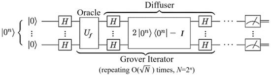
Figure 1.
The quantum circuit of Grover’s algorithm.
The oracle, denoted in Figure 1, plays a crucial role in identifying the target input by flipping its phase. Its definition is provided below.
In Equation (1), the target input is denoted . The oracle operates by flipping the phase of the state if and only if matches ; otherwise, it leaves the state unchanged.
The diffuser, on the other hand, is responsible for adjusting the probability amplitudes of quantum states by inverting them about their average value; it is an inversion around amplitude mean operation. Grover’s algorithm leverages the oracle and the diffuser to iteratively refine the quantum state of the system. Initially, the qubits are prepared in a uniform superposition state. When the oracle is applied, it flips the phase of the target input, effectively assigning it a negative probability amplitude. The diffuser then amplifies the amplitude of the target input and meanwhile reduces the amplitudes of all other inputs. Repeating the Grover iterator times significantly increases the amplitude of the target input while diminishing those of non-target inputs, allowing for the algorithm to identify the solution with high probability. Grover’s algorithm, which repeats the oracle and the diffuser O() times, has been shown in [8] to be the optimal oracle-based quantum search algorithm.
Grover’s algorithm can also handle scenarios involving multiple target inputs. In 1998, Boyer et al. demonstrated that when M target solutions exist and M is known beforehand, performing the oracle and the diffuser times ensures that all solutions can be identified with high probability. To estimate the number of solutions M in a given problem, Brassard et al. introduced the quantum counting algorithm in [13]. This algorithm employs quantum phase estimation (QPE) with t counting qubits and a total of Grover iterator repetitions [14]. However, this approach may result in large gate counts and deep quantum circuits, posing challenges for practical implementation.
Numerous research papers [12,15,16,17,18,19,20,21,22,23,24] are proposed in the literature to build quantum circuits based on Grover’s algorithm to solve various NP-hard and NP-complete problems. The solved problems include the k-coloring problem, the maximum clique problem, the list coloring problem, the pure Nash equilibria finding problem in graphical games, the Hamiltonian cycle problem, the dominating set problem, the exact cover problem, and the vertex cover problem. Readers are referred to [12] for descriptions of all the above-mentioned research results.
2.2. The Vertex Cover Problem
The vertex cover problem (VCP) is a well-known decision problem. It is also known as the k-vertex cover problem (k-VCP). As shown in [9], the VCP is NP-complete (NPC), meaning it is unlikely that a classical algorithm exists to solve it in polynomial time for any cases.
The problem definition is as follows. Given an undirected graph with n vertices and m edges, the k-VCP or the VCP associated with asks whether there exists a vertex subset with such that every edge is covered by , i.e., and/or . In this context, a vertex subset is called a k-vertex cover (or a vertex cover with size k) if its size is k and covers all edges in the graph. Simply put, the k-VCP determines whether a vertex cover of size k or smaller exists for a given graph. If so, it answers “yes”; otherwise, it outputs “no”.
For example, Figure 2 illustrates two vertex covers with size 2 for an undirected graph with 5 vertices and 4 edges. In the case of , the output of the k-VCP for this graph is “no”. However, in the case of , the output of the k-VCP for this graph is “yes”. For another example, Figure 3 illustrates three vertex covers with size 3 for an undirected graph with 7 vertices and 7 edges. In the cases of and , the output of the k-VCP for this graph is “no”. However, in the case of , the output of the k-VCP for this graph is “yes”.
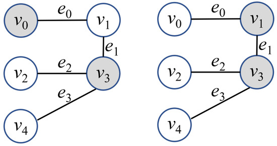
Figure 2.
Two vertex covers for an undirected graph with five vertices and four edges: (left) the vertex subset is a 2-vertex cover; (right) the vertex subset is also a 2-vertex cover.
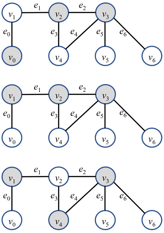
Figure 3.
Three vertex covers for an undirected graph with seven vertices and seven edges: (top) the vertex subset is a 3-vertex cover; (middle) the vertex subset is another 3-vertex cover; (bottom) the vertex subset is yet another 3-vertex cover.
The original VCP or k-VCP is a decision problem that determines whether a given graph has a vertex cover of size k or smaller. However, this paper also considers the search-version k-VCP, which outputs all vertex covers of size k (i.e., all k-vertex covers) for a given graph. Throughout this work, the term “k-VCP” may refer to either the decision version k-VCP or the search version k-VCP, depending on the context.
2.3. The Dicke State
The concept of Dicke states was introduced by Dicke in 1954 [25]. A Dicke state, denoted , is a special type of entangled quantum state of n qubits, where exactly k qubits are in and the rest are in . In other words, it is the equal (or symmetric) superposition of all n-qubit states with Hamming weight wt(x) = k, where wt(x) stands for the number of bits set to 1 in binary string x [26]. The Dicke state is defined as follows:
The number D of possible in-superposition states in is . For example, is an equal superposition of states.
For , can be considered as a constant. We therefore obtain the following Equation (3):
In Equation (3), for . By Equation (3), grows polynomially with n for . However, for k near , reaches its maximum value. By using Stirling’s approximation for factorials (i.e., ) [27], we have the following Equation (4):
In Equation (4), grows exponentially in n, with a polynomial correction factor of for . In summary, D grows polynomial with n, as long as , i.e., either or . In contrast, D grows exponentially with n when . For intermediate k, D transits between polynomial and exponential growth, depending on . It is notable that is required for the proposed DSQS algorithm to solve problems in polynomial time with bounded error. Therefore, we assume in this paper when k is not specified.
Generating Dicke states deterministically is a challenging task. In [26], Bartschi and Eidenbenz proposed a quantum circuit capable of efficiently preparing the Dicke state . This quantum circuit requires O quantum gates, has a depth of O, does not rely on ancillary qubits, and is compatible with the linear nearest neighbor (LNN) architecture. The overall circuit is based on a recursive decomposition based on an initial state to produce the final state . The recursive decomposition is described in Equation (5) as follows.
Equation (5) indicates that the preparation of can be achieved by combining the state along with and the state along with , while applying appropriate Y-rotation transforms to adjust the probability amplitudes.
By the recursive decomposition, Bartschi and Eidenbenz showed that the Dicke state preparation quantum circuit can be built based on two basic constructs, as depicted in Figure 4. Note that the boundary condition of the Dicke state decomposition is and . Also note that a Y-rotation gate transforms the state to the state to make qubits have proper probability amplitudes obeying the Dicke state superposition.
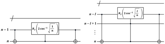
Figure 4.
The two basic constructs used to build the Dicke state preparation quantum circuit.
Figure 5 shows the quantum circuit using the two basic constructs recursively for Dicke state preparation. Figure 6 shows the quantum circuit implemented with IBM Qiskit packages to generate the Dicke state . Figure 7 shows the quantum circuit to measure qubits in the Dicke state . Figure 8 shows the measurement results of the quantum circuit of the Dicke state . From the measurement results, we can observe that qubits are in equal (or symmetric) superposition of states , and with the probability amplitude of and the probability density of .
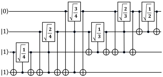
Figure 5.
An example of the quantum circuit for the Dicke state preparation, where a gate is a shorthand for a Y-rotation gate.
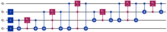
Figure 6.
The quantum circuit implemented with IBM Qiskit packages to generate the Dicke state .
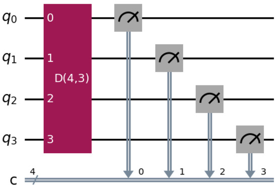
Figure 7.
The quantum circuit implemented with IBM Qiskit packages to measure qubits in the Dicke state .
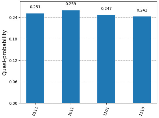
Figure 8.
The measurement results of the quantum circuit of the Dicke state .
3. DSQS
3.1. The DSQS Quantum Circuit
Figure 9 shows the quantum circuit of the proposed DSQS algorithm. As shown in Figure 9, the quantum circuit uses qubits, a Dicke state preparation gate and an oracle . All qubits are in initially. They include n working qubits (or input qubits) grouped as register x, one response qubit (or decision qubit) y as register y, and n mirror qubits grouped as register to reflect the states of qubits in register x.
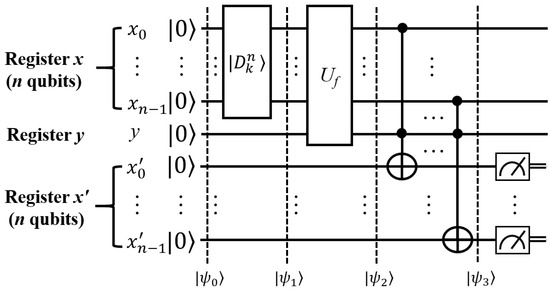
Figure 9.
The quantum circuit of the proposed Dicke state quantum search (DSQS) algorithm.
Initially, n working qubits in are used to span the search space. They are transformed into the Dicke state with a Dicke state gate. The resulting state is an equal superposition of states where exactly k qubits are in , and the remaining qubits are in . The total number of such possible in-superposition states is . Subsequently, the oracle is applied to the working qubits in register x and the qubit y in register y, performing the unitary transformation of the oracle as defined in the next subsection.
3.2. The DSQS Oracle
The DSQS oracle is a unitary transform that operates on the n working qubits (or input qubits) in register x and the decision qubit y in register y. Let T be the set of all target inputs or solutions to a given problem, and let be the function corresponding to the oracle for the given problem to satisfy the following definition:
The oracle is then defined as
When , the equation simplifies to
Specifically, the initial state of qubit y is . If the quantum state of the working qubits in register x corresponds to a target input or solution in set T, then the oracle sets qubit y to . Otherwise, qubit y remains .
Let the total number of solutions be M. Therefore, there are M states of register x matching with solution states corresponding to target inputs in T. Before the oracle operation , qubits are in the Dicke state in equal superposition of a total of possible states, and qubit y is . Therefore, the oracle flips the state of y to for M solution states out of the D states of , while leaving y in state for the remaining non-solution states. We therefore have the following Equation (9):
In Equation (9), we have that the probability amplitude of qubit y being is . Thus, the probability density P of qubit y being is . We then obtain the following equation:
We can measure register y to estimate the probability density P of y being . Let the estimated probability density be . According to Equation (10), we can estimate the total number of solutions M by multiplying with D, as shown in Equation (11).
In Equation (11), we can see that if the DSQS quantum circuit consists only of register x with n qubits and register y with a single qubit, it can also function as a quantum circuit for estimating the total number of solutions M.
However, DSQS performs more tasks, as described below. DSQS takes a qubit from register x and the qubit y as the two control qubits of a Toffoli, or controlled–controlled-X (CCX, or C2X) gate, with one qubit from register as the target qubit, where . This setup ensures that the solution states of register x of n working qubits are reflected on register of n mirror qubits , whereas the non-solution states are all reflected as on mirror qubits.
By measuring the results of register , we can identify the solutions to the given search problem. If the measurement outcome is the all-zero state with a probability of 1, it indicates that the problem has no solution. Conversely, non-all-zero outcomes, each occurring with a probability of , correspond to valid solutions to the problem. Meanwhile, the all-zero state occurs with a probability of , where M is the number of solutions and is the number of possible states in the Dicke state . The correctness of DSQS will be demonstrated in the next subsection.
3.3. The DSQS Correctness
The correctness for the DSQS quantum circuit using the Dicke state with states in superposition to identify all solutions to a given problem is proven by the unitary transformations below. Refer to Figure 9 for the placement of quantum states within the quantum circuit. Note that we use as the shorthand for .
In Equation (15), CCXi stands for a CCX gate with qubits and y as control qubits and with as the target qubit. In Equation (15), different registers are entangled. Therefore, measuring only a subset of registers (e.g., ) and discarding the rest is formally equivalent to taking a partial trace over the unmeasured registers. In Equation (16), for register in state (denoted ), its probability amplitude of is , and its probability amplitude of is , where , and T is the set of all M target inputs or solutions. Therefore, DSQS makes register have a probability density of for each solution state corresponding to a solution, and a probability density of for the all-zero state . If the problem has no solution, i.e., , the all-zero state has a probability density of .
3.4. The DSQS Error Probability
Bernstein and Vazirani introduced the complexity class of bounded-error quantum polynomial time (BQP) [28] in 1993. Specifically, BQP is defined as the class of decision problems solvable by a quantum Turing machine (QTM) [29] in polynomial time with an error probability that is less than 1/3. The QTM [29] was proposed by Deutsch in 1985; it is a quantum version of the classical Turing machine (TM) [30] proposed by Turing in 1936. A classical computer can be considered a TM, whereas a quantum computer is a QTM. Note that the error bound of 1/3 in BQP originates from the convention adopted by the classical probabilistic complexity class BPP (bounded-error probabilistic polynomial time) [31]. The choice of 1/3 is not mandatory. In practice, any constant less than 1/2 can be used, as it guarantees a success probability greater than 1/2. This is important because when the success probability exceeds 1/2, it can be boosted arbitrarily close to 1 by repeating the algorithm and taking a majority vote.
The Chernoff bound shows that the probability of majority error decreases exponentially in the number of repetitions.
Some algorithms, such as Shor’s algorithm, are believed to place problems, such as integer factorization and discrete logarithms, in BQP because the algorithms run in polynomial time to solve problems with bounded error on a quantum computer. While Grover’s algorithm also operates with bounded error, it does not place problems in BQP. This is because Grover’s algorithm finds all solutions to a problem among input instances by calling the oracle and diffuser O() times. The number of calls is exponential in the input size n, where n is the number of qubits defining the search space.
With the help of Dicke state , the proposed DSQS algorithm can locate all solutions of specific patterns to a given problem among input instances by calling only the oracle just once. However, it still does not place problems in BQP. This is because the probability of error not to locate a single solution is , which is not less than 1/3, where . Nonetheless, we show below that DSQS can locate all solutions with a probability of error less than 1/3 by performing O() repetitions, the order of which is polynomial, as long as .
As previously mentioned, the proposed DSQS does not utilize a diffuser for amplitude amplification. Instead, it maintains the probability amplitude of a solution state corresponding to a solution to be . This results in a probability density of for a solution state. Therefore, all solution states have the probability amplitude of with the probability density of . In contrast, a non-solution state corresponding to a non-solution has a probability amplitude and a probability density of 0, with the exception that the all-zero state has a probability amplitude of and the probability density of . Here, we assume the all-zero state is also a non-solution state without loss of generality. In practice, DSQS completely shifts the probability amplitudes of all non-solution states to the all-zero state. Thus, when we run DSQS and perform a single measurement, each solution state has, independently, a probability of being observed, whereas the all-zero state has a probability of being observed and the other non-solution states have no probability of being observed. Consequently, in the absence of noise, any measured result other than the all-zero combination can be considered a reflection of a solution.
Due to the Dicke state, the size of the search space for oracle processing is reduced from to for . This reduction allows for DSQS to ensure that the probability of not observing a single solution is smaller than after a polynomial number of repetitions. We present the following lemma and theorem:
Theorem 1.
The probability that a single solution is not observed by DSQS using the Dicke state becomes less than after O repetitions for .
Proof.
The probability that a single solution is observed in one repetition of DSQS using Dicke state is , where for . The probability of error that a single solution is not observed in one repetition of DSQS is therefore . Since for , we assume with c being a positive constant. Without loss of generality, we assume for .
Let be the probability of error that a single solution is not observed in t consecutive repetitions of DSQS. We obtain
We aim for , leading to
Taking the natural logarithm on both sides, we obtain
Substituting into , we obtain
The above equation derivation uses the Taylor expansion approximation, , where we assume for large n and higher-order terms are negligible. Thus, we obtain
Here, for and .
The above derivation shows that after repetitions of DSQS using the Dicke state , the probability that a single solution is not observed is less than for . □
4. DSQS-VCP
In this section, we present an algorithm to generate a quantum circuit based on DSQS using Dicke states to solve the k-VCP. The algorithm is named DSQS-VCP, and the generated quantum circuit is referred to as the DSQS-VCP quantum circuit. Below, we first introduce the DSQS-VCP algorithm and then present its complexity analysis.
4.1. The DSQS-VCP Algorithm
The DSQS-VCP algorithm, whose pseudo-code is shown in Algorithm 1 below, can generate a quantum circuit based on DSQS using the Dicke state to solve the k-VCP by finding all k-vertex covers for a given undirected graph , where the vertex set is of size n and the edge set is of size m. The quantum circuit is designed to identify all vertex covers of size k for the graph G.
The DSQS-VCP algorithm first prepares a quantum circuit containing qubits in initially. The qubits consist of n working qubits , grouped into a register x, with each qubit corresponding to a vertex in V. also contains qubits serving as qubits associated with the controlled quantum flag (CQF) gates used by the m edges, where each edge uses two qubits for its associated quantum flag gates, as will be explained later. In addition, contains a qubit y as a register y, and n mirror qubits , grouped into a register , as well as n classical bits grouped as to store the measurement results of mirror qubits.
First of all, applies a gate to working qubits to make them in the Dicke state . Note that the gate may be labeled as D() in practical implementations later. Afterwards, employs many CQF gates, as introduced below. The CQF gate is inspired by the concept of controlled quantum semaphore (CQS) gate proposed in [22]. The function of the CQF gate, which has two flag qubits, is to verify whether a given vertex subset S, specified by the state of register x, covers a specific edge , that is, to check whether and/or . If so, the first flag qubit, which is initially , will be flipped to ; otherwise, it remains in . Note that the second flag qubit functions merely as an ancillary qubit to assist the first flag qubit to be set properly.
Figure 10 shows the block diagram of the CQF gate along with its detailed quantum circuit. The CQF gate, denoted Flag in Figure 10, has one control qubit, , and two flag qubits, and , all initially in . Table 1 shows all the possible combinations of gate inputs (i.e., , , and ) and gate outputs (i.e., , , and ) of the gate. Note that initially and always remains in , so there is no input combination of in Table 1. On the contrary, remains unchanged if is , and it is definitely if is . The CQF gate is synthesized directly from the truth table with the fewest possible qubits and MCX gates.
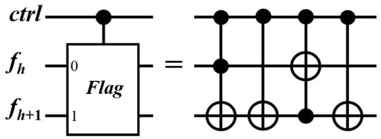
Figure 10.
(left) Block diagram of a CQF gate, denoted Flag, and (right) its detailed quantum circuit.

Table 1.
State transition of a CQF gate, , with as the control qubit.
An edge uses two consecutive CQF gates with flag qubits and , as well as control qubits and , as shown in Figure 11. Note that the two flag qubits are in initially. The possible states of and are shown in Table 2. The reader can verify that if the control qubit is , then both qubits and remain in . In contrast, if the control qubit is , then both qubits and are first set to . Afterwards, qubit is reset to by an X gate. Consequently, if the CQF gate is applied again with the control qubit in , then qubit is set to and is first set to and then reset to . Specifically, starting from the initial state of , the flag qubit finally remains in only if and . For the case of and and the cases of either or , the flag qubit is definitely in . Note that (resp., ) means that vertex (resp., ) is included in the vertex subset corresponding to the state of the working qubits. So, we just check whether the flag qubit is or not. If is , then the edge e is covered by and/or .
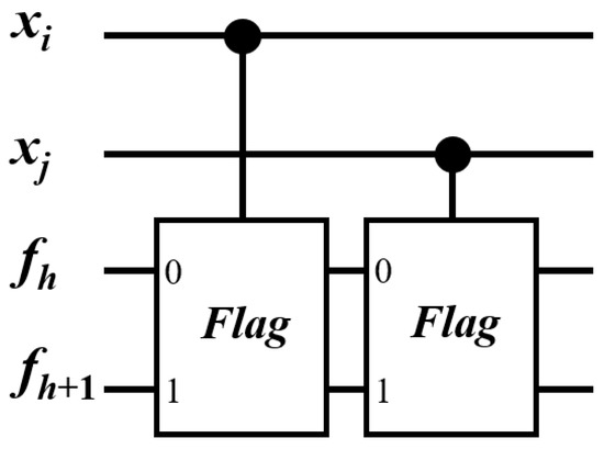
Figure 11.
Two consecutive CQF (or Flag) gates using two flag qubits and are employed to check if an edge is covered by vertex and/or vertex , where (resp., ) of indicates that (resp., ) is included in the vertex subset corresponding to the state of working qubits.
Table 2.
State transition of two consecutive CQF gates, , with and as the first and the second control qubits, respectively.
After using CQF gates to check if each of m edges is covered by at least one vertex, employs an MCX gate to check if all edges are covered by at least one vertex. The MCX gate takes the flag qubits as control qubits and takes the response qubit y as the target qubit. Therefore, if all edges are covered by at least one vertex, then the response qubit y is , meaning that the associated quantum state corresponds to a solution (i.e., a k-vertex cover) of the given k-VCP. Afterwards, n CCX gates are used to reflect the state of qubit on qubit with the ith CCX gate taking qubit and qubit y as the control qubits and taking qubit as the target qubit, where .
Finally, measuring the n mirror qubits can reveal the solutions to the given k-VCP. If the measurement results are all zeros with probability 1, then the k-VCP has no solution. Otherwise, any non-all-zero result is a solution to the given k-VCP. As described earlier, if there are M solutions, then each non-all-zero measurement result is supposed to have a probability of to be observed, and the all-zero measurement result is obtained, , where for .
| Algorithm 1: DSQS-VCP |
| Input: A k-vertex cover problem (k-VCP) instance: a given positive integer k and a given undirected graph , where the vertex set is of size n and the edge set is of size m. Output:: QC: a quantum circuit based on DSQS using the Dicke state to solve the k-VCP
|
4.2. The DSQS-VCP Complexity Analysis
Below, we analyze the time complexity of the DSQS-VCP algorithm. First of all, DSQS-VCP applies a gate to working qubits. According to [26], a gate has O() basis gates, which implies that the time complexity to add the O() basis gates in the quantum circuit to realize the gate is also O(). Then, we analyze the other parts of DSQS-VCP. The most computationally intensive part of DSQS-VCP lies in two main loops. The first loop adds two consecutive CQF gates for every edge of totally m edges. The time complexity of the first loop is O(m). The second loop adds a CCX gate for every vertex of totally n vertices. The time complexity of the second loop is O(n). Thus, the total time complexity of the two DSQS-VCP main loops is O. Consequently, the overall time complexity of DSQS-VCP to generate a quantum circuit is O, which is polynomial.
Below, we analyze the circuit complexity of the DSQS-VCP quantum circuit in terms of the qubit count, gate count, and circuit depth. In general, uses qubits, including n working qubits of register x, a total of flag qubits of CQF gates, a qubit y of register y, and n mirror qubits of register .
We first analyze the number of quantum gates and the circuit depth. The high-level gates are a gate, CQF gates, an m-control-qubit Toffoli (CmX) gate, and n CCX (C2X) gates. According to [26], a gate costs O() gates and O(n) depth. Based on Figure 10, a CQF gate uses two CX gates and two X gates with constant depth inside the CQF gate quantum circuit. Thus, CQF gates cost O(m) gates and O(m) depth.
Below, we analyze the CmX gate and the n C2X gates. Numerous studies have tried to decompose the CmX gate into gates in a selected universal basis gate set. Note that a universal basis gate set is a finite set of quantum gates that can be combined to approximate any quantum operation (or gate). For example, the set of an H gate, a T gate, and a CX gate (i.e., H, T, CX) is a widely used universal basis gate set. The authors in [32] selected H, T, and CX gates as the basis gates to decompose a CmX gate into = O(m) T gates and = O(m) CX gates with the circuit depth = O(m), along with an extra ancilla qubit. The authors in [33] show that a CCX gate can be decomposed into a constant number of H, T, and CX gates without any extra ancilla qubit with a constant depth. Therefore, the CmX gate and the n C2X gates cost O() basis gates and O() depth with an extra ancilla qubit.
From all of the above-mentioned analysis results, we conclude that the DSQS-VCP quantum circuit uses totally = O() qubits and O() gates with O() depth. We can see that the qubit count, the gate count, and the circuit depth of are all polynomial.
Constructing quantum circuits to solve intractable problems, particularly NPC problems such as the k-VCP, is challenging due to the need to encode combinatorial constraints into oracle operations, often resulting in high complexity in terms of qubit usage, gate count, and circuit depth. The DSQS-VCP algorithm proposed in this section addresses this challenge by systematically generating a DSQS-based quantum circuit for solving instances of the k-VCP. Our analysis demonstrates that the resulting quantum circuit, including the oracle component that enforces the problem constraints, has a polynomial complexity with respect to the problem size in terms of construction time complexity, qubit usage, gate counts, and circuit depth. Notably, a significant portion of the overall circuit corresponds to the oracle implementation. This highlights the practical advantage of the DSQS algorithm, which requires only a single oracle invocation per execution, effectively reducing the cumulative cost associated with complex oracle constructions and their repetitions.
5. Experimental Results
This section shows two experiments using IBM Qiksit packages to implement and run DSQS-VCP quantum circuits based on DSQS using the Dicke state to successfully find all solutions to given k-VCP instances. The experiments rely on IBM Aer Simulator with or 5000 shots (repetitions) per experiment, where n is the number of input qubits. Since this paper primarily addresses the proof of principle and complexity analysis of DSQS and DSQS-VCP, we do not conduct experiments to execute DSQS-VCP quantum circuits on real quantum computers. The details of the experiments are described in the following subsections.
5.1. The First Experiment
The first experiment is to implement and run the DSQS-VCP quantum circuit to find all solutions to the k-VCP defined below. Given an undirected graph with vertices in V and edges in E, as shown in Figure 2, the k-VCP is associated with different k values, such as 1, 2, and 3.
Figure 12 shows the DSQS-VCP quantum circuit to find all solutions to the k-VCP with in the first experiment. The quantum circuit has working qubits for vertices in vertex set V. With a Dicke state preparation gate, the working qubits are set to state to form the space of possible input instances. Note that the quantum circuits for and are all the same, except that they use different Dicke state preparation gates. As mentioned earlier, an edge uses two consecutive CQF gates (denoted “Flag” gates in Figure 12) having two flag qubits and two different control qubits, and , to check whether the edge e is covered by and/or . For example, in the DSQS-VCP quantum circuit of the first experiment, two flag qubits and in are initially used to check the coverage of the edge by vertices and/or . It is required to check whether the flag qubit is or not to determine if edge is covered by and/or . The coverage of edges can be checked similarly.
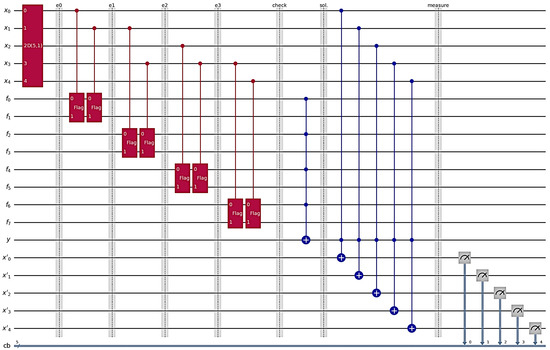
Figure 12.
The DSQS-VCP quantum circuit to find all solutions to the k-VCP in the first experiment.
The decision qubit y, which is initially , then serves as the target qubit of an MCX gate that takes the first flag qubit of all quantum flag gates as its control qubits. Therefore, if all of the first flag qubits are , then qubit y is flipped from to . This means that the bit combination corresponding to the quantum state is a solution to the given k-VCP.
Afterwards, CCX gates, each of which takes qubits y and as two control qubits and qubit as the target qubit, are appended to the quantum circuit. This is intended to reflect the quantum states of working qubits corresponding to solutions on mirror qubits , where . Therefore, the mirror qubits are in the superposition of all quantum states corresponding to all M solutions and the state . It is notable that the quantum state corresponding to a solution has a probability amplitude of and the quantum state has a probability amplitude of , where . It is easy to check whether the given k-VCP has no solution. If so, the mirror qubits are definitely in with a probability amplitude of 1.
Figure 13, Figure 14 and Figure 15 show the histogram of the measurement results of the DSQS-VCP quantum circuit to find all solutions to the k-VCP for k = 1, 2, and 3 in the first experiment. In Figure 13, there is only one outcome 00000 with a probability of 1 for with either shots or 5000 shots, which means the k-VCP has no solution for the case of k = 1. Note that we only present one diagram in Figure 13, as diagrams with 5 shots and 5000 shots are the same.
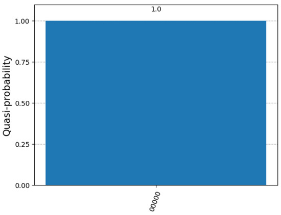
Figure 13.
Histogram of the measurement results of the DSQS-VCP quantum circuit to find all solutions to the k-VCP for with and 5000 shots in the first experiment.
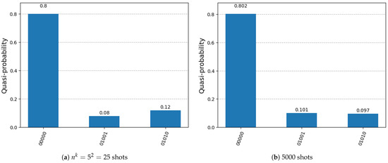
Figure 14.
Histogram of the measurement results of the DSQS-VCP quantum circuit to find all solutions to the k-VCP for in the first experiment.
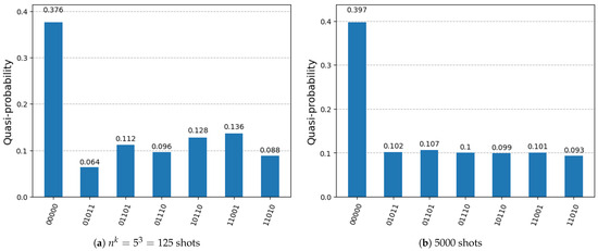
Figure 15.
Histogram of the measurement results of the DSQS-VCP quantum circuit to find all solutions to the k-VCP for in the first experiment.
From Figure 14a,b, we can observe that there are outcomes, 10001 and 10100, with probabilities of approximately for shots and 5000 shots, where . More shots lead to probabilities that are closer to . Specifically, they correspond to two solutions, and , to the given k-VCP for k = 2. The solutions correspond to two-vertex covers of the graph in the given k-VCP. There are totally non-solutions among input instances, indicated by the outcome 00000 with a probability that is approximately .
From Figure 15a,b, we can observe that there are outcomes, 01110, 10011, 10101, 10110, 11001, and 11100, with probabilities of approximately for shots and 5000 shots, where . More shots lead to probabilities that are closer to . Specifically, they correspond to all the six three-vertex covers of the graph in the given k-VCP. There are, in total, non-solutions among input instances, indicated by the outcome 00000, with a probability of approximately .
5.2. The Second Experiment
The second experiment is to implement and run the DSQS-VCP quantum circuit to find all solutions to the k-VCP defined below. Given a undirected graph with vertices in V and edges in E, as shown in Figure 3, the k-VCP is associated with different k values, such as 2, 3, and 4.
Figure 16 shows the DSQS-VCP quantum circuit to find all solutions to the k-VCP with in the second experiment. The quantum circuit has working qubits for vertices in vertex set V. With a Dicke state preparation gate, the working qubits are set to state to form the space of possible input instances. Note that the quantum circuits for and are all the same, except that they use different Dicke state preparation gates. As mentioned earlier, an edge uses two consecutive CQF gates (denoted “Flag” gates in Figure 16) having two flag qubits and two different control qubits, and , to check whether the edge e is covered by and/or , where . For example, in the DSQS-VCP quantum circuit of the second experiment, two flag qubits, and in , initially are used to check the coverage of edge by vertices and/or . It is required to check whether the flag qubit is or not to determine if edge is covered by and/or . The coverage of edges can be checked similarly.
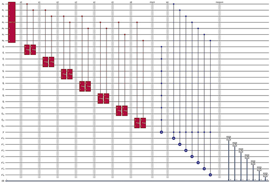
Figure 16.
The DSQS-VCP quantum circuit to find all solutions to the k-VCP in the second experiment.
The decision qubit y, which is initially , then serves as the target qubit of an MCX gate that takes the first flag qubit of all quantum flag gates as its control qubits. Therefore, if all of the first flag qubits are , then qubit y is flipped from to . This means that the bit combination corresponding to the quantum state is a solution to the given k-VCP.
Afterwards, CCX gates, each of which takes qubits y and as two control qubits and qubit as the target qubit, are appended into the quantum circuit. This is intended to reflect the quantum states of working qubits corresponding to solutions into mirror qubits , where . Therefore, the mirror qubits are in the superposition of all quantum states corresponding to all M solutions and the state . It is notable that the quantum state corresponding to a solution has a probability amplitude of and the quantum state has a probability amplitude of , where . It is easy to check whether the given k-VCP has no solution. If so, the mirror qubits are definitely in with a probability amplitude of 1.
Figure 17, Figure 18 and Figure 19 show histograms of the measurement results of the DSQS-VCP quantum circuit to find all solutions to the k-VCP for k = 2, 3, and 4 in the second experiment. In Figure 17, there is only one outcome, 0000000, with a probability of 1 for with either shots or 5000 shots, which means the k-VCP has no solution for the case of k = 2. Note that we only present one diagram in Figure 17, as diagrams with 49 shots and 5000 shots are the same.

Figure 17.
Histogram of the measurement results of the DSQS-VCP quantum circuit to find all solutions to the k-VCP for with and 5000 shots in the second experiment.
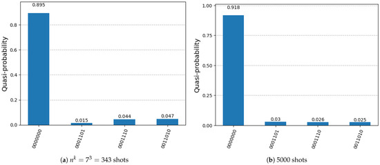
Figure 18.
Histogram of the measurement results of the DSQS-VCP quantum circuit to find all solutions to the k-VCP for in the second experiment.
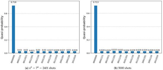
Figure 19.
Histogram of the measurement results of the DSQS-VCP quantum circuit to find all solutions to the k-VCP for in the second experiment.
In Figure 18a,b, we can observe that there are outcomes, 0001101, 0001110, and 0011010, with probabilities of approximately . More shots lead to probabilities that are closer to . Specifically, they correspond to three solutions, , , and , to the given k-VCP for k = 3. The solutions correspond to three-vertex covers of the graph in the given k-VCP. There are a total of non-solutions among input instances, indicated by the outcome 0000000 with a probability of approximately .
In Figure 19a,b, we can observe that there are outcomes, 0001111, 0011011, 0011101, 0011110, 0101101, 0101110, 0111010, 1001101, 1001110, and 1011010, with probabilities of approximately . More shots lead to probabilities closer to . Specifically, they correspond to all the ten four-vertex covers of the graph in the given k-VCP. There are, in total, non-solutions among input instances, indicated by the outcome 0000000, with a probability of approximately .
6. Conclusions
This paper first proposes a quantum search algorithm, named DSQS, as a general quantum algorithm to set qubits in the Dicke state to identify all target inputs or solutions of specific patterns from unstructured input instances by calling an oracle only once. DSQS improves Grover’s algorithm, which needs to repeat an oracle and a diffuser times to find all M solutions out of inputs with high probability, where n is the number of input qubits to span the search space. Furthermore, Grover’s algorithm requires prior knowledge of the number M of solutions, whereas DSQS operates without this prerequisite. We prove the correctness of DSQS by unitary transformations and show that DSQS can locate every single solution with an error probability less than 1/3 through O() repetitions for .
Our research result does not conflict with the assertion that Grover’s algorithm is the optimal oracle-based quantum search algorithm. This is because that DSQS sets qubits into the Dicke state of D in superposition states, reducing the number of search states for the oracle to be under the condition of . Grover’s algorithm calls an oracle and the diffuser O() times to find solutions with high probability through one repetition. In contrast, DSQS calls an oracle once to locate solutions with a probability of through one repetition. Afterwards, DSQS can locate solutions with high probability through O() repetitions for .
This paper also proposes a classical algorithm, named DSQS-VCP, to generate a quantum circuit based on DSQS using the Dicke state to solve the search version k-VCP by locating all solutions to the k-VCP. We analyze the time complexity of DSQS-VCP and decompose its generated quantum circuit into components consisting of only H, T, and CX gates, which are basis gates of a universal gate set. This decomposed circuit is shown to have a polynomial qubit count, gate count, and circuit depth. The overall complexity analysis reveals that DSQS-VCP can generate a quantum circuit based on DSQS using the Dicke state to find all k-VCP solutions in polynomial time with a probability of error less than 1/3 for . Since the k-VCP is NP-complete, NP and NPC problems can be polynomially reduced to the k-VCP. If the reduced k-VCP instance satisfies , then both the instance and the original NP/NPC problem instance to which it corresponds can be solved by the DSQS-VCP quantum circuit in polynomial time with an error probability less than 1/3.
We conducted experiments using IBM Qiskit packages to implement and run the proposed QSDS-VCP quantum circuits, successfully identifying all solutions to the example k-VCP instances. The instances are for small n and k, such as and , all of which satisfy the condition . However, these experiments were performed using IBM Qiskit simulators and do not consider real-device conditions such as qubit decoherence, gate noise, or connectivity constraints. As this paper focuses on theoretical aspects and proof of principle, experiments on real quantum computers were not conducted. In the future, we plan to extend this work with implementations on real quantum computers and conduct detailed error resilience analysis to assess the algorithm’s performance under realistic noise models. Additionally, we intend to continue exploring theoretical aspects, particularly investigating how to use the first half of the DSQS quantum circuit that contains only registers x and y to estimate the total number M of solutions. We aim to derive the error bound of the estimation of M and then determine the minimum number of repetitions required for DSQS to identify all M solutions with high probability. Furthermore, we plan to explore whether certain NP and NPC problems can be reduced to k-VCP satisfying , so that they can be solved in polynomial time with an error probability less than 1/3 via the DSQS-VCP quantum circuit. We also seek to design algorithms similar to DSQS-VCP to directly generate quantum circuits based on DSQS using the Dicke state for solving certain NP and NPC problems in polynomial time with an error probability less than 1/3 for .
The paper [34] proposes an improved Grover’s algorithm by using a diffuser tailored for the Dicke state to exploit quantum interference for amplifying the probability amplitudes of the solution states. In the Dicke state , the number of in-superposition states is given by , which is of under the condition of . Therefore, a total of Grover iterators, each of which is composed of an oracle and a diffuser, are required to find all M solutions with high probability. This reduces the required repetitions of the Grover iterator from O() in the original Grover’s algorithm to only O() as long as . However, the improved Grover’s algorithm still requires prior knowledge of the number M of solutions to accurately determine the optimal number R of Grover iterator repetitions. According to [7], Grover’s algorithm suffers from the “overshooting problem”, in which repeating the Grover iterator over R times causes the probability amplitudes of the solution states to decrease.
In the future, we plan to integrate the improved Grover’s algorithm proposed in [34] with the DSQS algorithm proposed in this paper to leverage the advantages of both methods. The basic idea of the integrated method is to initially assume an estimated number of solutions, where . With , we can then assume an estimated optimal number of Grover iterator repetitions without knowing the exact value of M. When , we have . Thus, we can repeat the Grover iterator only times, where , not only to reduce the quantum circuit depth and the number of quantum gates used, but also to avoid the overshooting problem. After that, we apply the special oracle of the DSQS algorithm and then determine all solutions through a suitable number of measurements. Because the diffuser amplifies the amplitudes of the solution states, the number of measurements or shots required is reduced. We will analytically derive the appropriate number of measurements by examining the amplitude amplification induced by the diffuser and conduct experiments to validate our analysis. We will also design an adaptive algorithm that assumes successive estimated values of the number of solutions, , from larger to smaller. Consequently, the corresponding values of increases, but the required number of measurements decreases gradually. The adaptive algorithm stops when the number of identified solutions exceeds , enabling the integrated method to adaptively and efficiently identify solutions. This aims to pursue a resource-efficient optimization objective: reduce the number of Grover iterator repetitions as much as possible and, at the same time, minimize the number of shots required by the DSQS quantum circuit, all without prior knowledge of the number M of solutions.
While we have outlined the integration of DSQS with the improved Grover’s algorithm proposed in [34], we note that a rigorous theoretical or empirical comparison between the two standalone approaches has not yet been conducted. Such a comparison—especially in terms of the qubit count, gate count, circuit depth, and number of shots required to locate solutions—will be pursued in future work to better position the advantages and trade-offs of each algorithm.
Knowing the exact number M of solutions can benefit the improved Grover’s algorithm proposed in [34], as it allows for determining the appropriate number of Grover iterator repetitions to maximize the amplitude of the target states without causing amplitude overshooting. However, in many practical scenarios, M is unknown. One way to estimate M is by using the quantum counting algorithm [13], which requires Grover iterator repetitions when t counting qubits are used. Alternatively, we may estimate M by using only a portion of the DSQS quantum circuit proposed in this paper—specifically, the part consisting of the n-qubit register x, the single-qubit register y, one Dicke state preparation gate, one oracle, and the final measurement on the y register. Although a formal proof has not yet been established, it is expected that this partial DSQS circuit can estimate the value of M with low error probability after a number of measurements proportional to , which is and remains polynomial as long as the condition is satisfied. In the future, we plan to integrate this partial circuit with the amplitude amplification mechanism of the improved Grover’s algorithm proposed in [34] to further reduce the number of measurements required by the partial circuit for the solution count estimation. We will conduct an in-depth analysis of the relationship between the number of repetitions of the Grover iterator and the number of measurements needed to accurately determine the solution count. The goal of this integration is to perform a small number of Grover iterations while allowing for the partial circuit to accurately estimate the solution count with significantly fewer measurements.
We briefly recall that BQP (Bounded-error Quantum Polynomial time) is the class of decision problems solvable by a family of polynomial complexity quantum Turing machines (quantum circuits) with error bounded by a constant (e.g., a constant ) [14,28]. It is noted that all statements of polynomial complexity in this paper apply only to VCP instances and similar instances of other problems for which the feasible solution set lies in a fixed-Hamming-weight Dicke state subspace with a polynomial size of under the condition of . DSQS samples uniformly from that subspace of size D, yielding per-shot solution probability to observe a single solution. Consequently, the D = O repetition bound is required, which is not asymptotically better than exhaustive enumeration methods. The required shot budgets are therefore probabilistic demonstrations rather than certificates that all D candidates are examined. Nevertheless, DSQS may be combined with amplitude amplification algorithms confined to the Dicke state subspace, such as the improved Grover’s algorithm [34], to boost single-shot success probabilities of observing a solution. Appendix A shows shows the results of a preliminary experiment of the method combining DSQS with the improved Grover algorithm [34] using Dicke states. This experiment, using the same setting as Experiment 1 in Section 5, indicates that amplitude amplification can significantly enhance the probability of finding target solutions. Since the correctness of the combined method cannot be validated solely by this preliminary experiment, nor can the improvement in success probability be analytically established, we will conduct a comprehensive exploration covering theoretical derivations, probability analyses, and experiments across various scenarios. Our goal is to verify that DSQS can enhance the effectiveness of quantum search algorithms in locating target solutions.
Funding
This research was supported in part by the National Central University (NCU) and in part by the National Science and Technology Council (NSTC) under Grant 113-2622-E-008-019 and Grant 114-2119-M-006-006.
Data Availability Statement
Since the related technology described in the paper is currently under patent application, the data presented in this study are available on request from the corresponding author.
Acknowledgments
We express our gratitude to the National Taiwan University—IBM Quantum Computing Center (IBM Q Hub at NTU) for providing us with access to the IBM Q system.
Conflicts of Interest
The author declares no conflicts of interest.
Appendix A
This appendix shows the results of a preliminary experiment of the method combining DSQS with the Dicke state-based Grover’s algorithm [34] to find all solutions to the k-VCP. This preliminary experiment uses the same experimental setting as Experiment 1 in Section 5. Specifically, the experiment is to solve the k-VCP for an undirected graph with vertices in V and edges in E, as shown in Figure 2, with .
Figure A1 shows the quantum circuit to find all solutions to the k-VCP with . The quantum circuit has working qubits for vertices in vertex set V. With a Dicke state preparation gate, the working qubits are set to state to form the space of possible input instances. An edge uses two consecutive CQF gates (denoted “F” gates in Figure A1) having two flag qubits and two different control qubits, and , to check whether the edge e is covered by and/or . An ancilla qubit z, which is set to by an X gate and an H gate, then serves as the target qubit of an MCX gate that takes the first flag qubit of all quantum flag gates as its control qubits. Therefore, if all of the first flag qubits are , then qubit z is forced to trigger the phase kickback effect. The phase of the quantum state that makes the first flag qubit of all quantum flag gates is then reversed.
Afterwards, a series of inverse CQF gates (denoted “iF” gates in Figure A1) are applied in the reverse order of their corresponding CQF gates. The iF gates reset the flag qubits by uncomputing the auxiliary information, restoring them to and eliminating residual entanglement, thereby ensuring that only the edge cover constraints contribute to the subsequent amplitude amplification.
In the subsequent circuit, a diffuser confined to the Dicke state subspace is applied. According to [34], the diffuser is constructed by an iD(5,2) gate, n X gates, a gate, n X gates, and a D(5,2) gate, where iD(5,2) denotes the inverse Dicke state construction gate of . The diffuser performs a reflection about the mean of all states in the Dicke state subspace, ensuring that the amplitude amplification process is confined to the space spanned by .
The final part in the quantum circuit is the DSQS algorithm, which ensures that the measurement yields the states corresponding to the target solutions (whose amplitudes have already been amplified by the diffuser), while the non-solution states are all mapped to the all-zero state.
Figure A2 shows the histogram of the measurement results of the quantum circuit to find all solutions to the k-VCP with k = 2. We observe that, by leveraging the amplitude amplification of the improved Grover’s algorithm, the probability of finding a target solution can be significantly boosted.

Figure A1.
Quantum circuit of combining DSQS with the improved Grover’s algorithm using Dicke states to find all solutions to the k-VCP in the preliminary experiment.

Figure A2.
Histogram of the measurement results of the method that combining DSQS and improved Grover’s algorithm using Dicke states to find all solutions to the k-VCP for in the preliminary experiment.
References
- Jiang, J.R.; Chu, C.W. Classifying and benchmarking quantum annealing algorithms based on quadratic unconstrained binary optimization for solving NP-hard problems. IEEE Access 2023, 11, 104165–104178. [Google Scholar] [CrossRef]
- Jiang, J.R.; Shu, Y.C.; Lin, Q.Y. Benchmarks and Recommendations for Quantum, Digital, and GPU Annealers in Combinatorial Optimization. IEEE Access 2024, 12, 125014–125031. [Google Scholar] [CrossRef]
- Arute, F.; Arya, K.; Babbush, R.; Bacon, D.; Bardin, J.C.; Barends, R.; Biswas, R.; Boixo, S.; Brandao, F.G.; Buell, D.A.; et al. Quantum supremacy using a programmable superconducting processor. Nature 2019, 574, 505–510. [Google Scholar] [CrossRef] [PubMed]
- Deutsch, D.; Jozsa, R. Rapid solution of problems by quantum computation. Proc. R. Soc. Lond. Ser. A Math. Phys. Sci. 1992, 439, 553–558. [Google Scholar]
- Shor, P.W. Algorithms for quantum computation: Discrete logarithms and factoring. In Proceedings of the Proceedings 35th Annual Symposium on Foundations of Computer Science, Santa Fe, NM, USA, 20–22 November 1994; pp. 124–134. [Google Scholar]
- Grover, L.K. A fast quantum mechanical algorithm for database search. In Proceedings of the Twenty-Eighth Annual ACM Symposium on Theory of Computing, Philadelphia, PA, USA, 22–24 May 1996; pp. 212–219. [Google Scholar]
- Boyer, M.; Brassard, G.; Høyer, P.; Tapp, A. Tight bounds on quantum searching. Fortschritte Phys. Prog. Phys. 1998, 46, 493–505. [Google Scholar] [CrossRef]
- Bennett, C.H.; Bernstein, E.; Brassard, G.; Vazirani, U. Strengths and weaknesses of quantum computing. SIAM J. Comput. 1997, 26, 1510–1523. [Google Scholar] [CrossRef]
- Karp, R.M. Reducibility among Combinatorial Problems. In Proceedings of the Complexity of Computer Computations: Proceedings of a Symposium on the Complexity of Computer Computations, New York, NY, USA, 20–22 March 1972; pp. 85–103. [Google Scholar]
- Cook, S.A. The complexity of theorem-proving procedures. In Proceedings of the Third Annual ACM Symposium on Theory of Computing, Shaker Heights, OH, USA, 3–5 May 1971; pp. 151–158. [Google Scholar]
- Fadillah, M.H.A.Z.; Idrus, B.; Hasan, M.K. Introduction to IBM Quantum & Qiskit. 2021. Available online: https://ftsm.ukm.my/v5/file/research/technicalreport/LP-CAIT-FTSM-2021-010.pdf (accessed on 9 September 2025).
- Jiang, J.R.; Wang, Y.J. Using a Simplified Quantum Counter to Implement Quantum Circuits Based on Grover’s Algorithm to Tackle the Exact Cover Problem. Mathematics 2024, 13, 90. [Google Scholar] [CrossRef]
- Brassard, G.; Høyer, P.; Tapp, A. Quantum counting. In Proceedings of the Automata, Languages and Programming: 25th International Colloquium, ICALP’98, Aalborg, Denmark, 13–17 July 1998; Proceedings 25. Springer: Berlin/Heidelberg, Germany, 1998; pp. 820–831. [Google Scholar]
- Nielsen, M.A.; Chuang, I.L. Quantum Computation and Quantum Information; Cambridge University Press: Cambridge, UK, 2010. [Google Scholar]
- Saha, A.; Saha, D.; Chakrabarti, A. Circuit design for k-coloring problem and its implementation on near-term quantum devices. In Proceedings of the 2020 IEEE International Symposium on Smart Electronic Systems (iSES) (Formerly iNiS), Chennai, India, 14–16 December 2020; pp. 17–22. [Google Scholar]
- Saha, A.; Saha, D.; Chakrabarti, A. Circuit design for k-coloring problem and its implementation in any dimensional quantum system. SN Comput. Sci. 2021, 2, 427. [Google Scholar] [CrossRef]
- Haverly, A.; López, S. Implementation of Grover’s algorithm to solve the maximum clique problem. In Proceedings of the 2021 IEEE Computer Society Annual Symposium on VLSI (ISVLSI), Tampa, FL, USA, 7–9 July 2021; pp. 441–446. [Google Scholar]
- Mukherjee, S. A Grover search-based algorithm for the list coloring problem. IEEE Trans. Quantum Eng. 2022, 3, 3101008. [Google Scholar] [CrossRef]
- Roch, C.; Castillo, S.L.; Linnhoff-Popien, C. A Grover based quantum algorithm for finding pure Nash equilibria in graphical games. In Proceedings of the 2022 IEEE 19th International Conference on Software Architecture Companion (ICSA-C), Honolulu, HI, USA, 12–15 March 2022; pp. 147–151. [Google Scholar]
- Jiang, J.R. Quantum circuit based on Grover algorithm to solve Hamiltonian cycle problem. In Proceedings of the 2022 IEEE 4th Eurasia Conference on IOT, Communication and Engineering (ECICE), Yunlin, Taiwan, 28–30 October 2022; pp. 364–367. [Google Scholar]
- Jiang, J.R.; Kao, T.H. Solving Hamiltonian Cycle Problem with Grover’s Algorithm Using Novel Quantum Circuit Designs. In Proceedings of the 2023 IEEE 5th Eurasia Conference on IOT, Communication and Engineering (ECICE), Yunlin, Taiwan, 27–29 October 2023; pp. 796–801. [Google Scholar]
- Jiang, J.R.; Yan, W.H. Novel Quantum Circuit Designs for the Oracle of Grover’s Algorithm to Solve the Vertex Cover Problem. In Proceedings of the 2023 IEEE 5th Eurasia Conference on IOT, Communication and Engineering (ECICE), Yunlin, Taiwan, 27–29 October 2023; pp. 652–657. [Google Scholar]
- Jiang, J.R.; Wang, Y.J. Quantum circuit based on Grover’s algorithm to solve exact cover problem. In Proceedings of the 2023 VTS Asia Pacific Wireless Communications Symposium (APWCS), Tainan, Taiwan, 23–25 August 2023; pp. 1–5. [Google Scholar]
- Jiang, J.R.; Lin, Q.Y. Utilizing Novel Quantum Counters for Grover’s Algorithm to Solve the Dominating Set Problem. arXiv 2023, arXiv:2312.09388. [Google Scholar]
- Dicke, R.H. Coherence in spontaneous radiation processes. Phys. Rev. 1954, 93, 99. [Google Scholar] [CrossRef]
- Bärtschi, A.; Eidenbenz, S. Deterministic preparation of Dicke states. In Proceedings of the International Symposium on Fundamentals of Computation Theory, Copenhagen, Denmark, 12–14 August 2019; Springer: Berlin/Heidelberg, Germany, 2019; pp. 126–139. [Google Scholar]
- Knuth, D.E. The Art of Computer Programming: Fundamental Algorithms; Addison-Wesley Professional: Boston, MA, USA, 1997; Volume 1. [Google Scholar]
- Bernstein, E.; Vazirani, U. Quantum complexity theory. In Proceedings of the Twenty-Fifth Annual ACM Symposium on Theory of Computing, San Diego, CA, USA, 16–18 May 1993; pp. 11–20. [Google Scholar]
- Deutsch, D. Quantum theory, the Church–Turing principle and the universal quantum computer. Proc. R. Soc. Lond. A Math. Phys. Sci. 1985, 400, 97–117. [Google Scholar]
- Turing, A.M. On computable numbers, with an application to the Entscheidungs problem. J. Math 1936, 58, 5. [Google Scholar]
- Gill III, J.T. Computational complexity of probabilistic Turing machines. In Proceedings of the Sixth Annual ACM Symposium on Theory of Computing, Seattle, WA, USA, 30 April–2 May 1974; pp. 91–95. [Google Scholar]
- He, Y.; Luo, M.X.; Zhang, E.; Wang, H.K.; Wang, X.F. Decompositions of n-qubit Toffoli gates with linear circuit complexity. Int. J. Theor. Phys. 2017, 56, 2350–2361. [Google Scholar] [CrossRef]
- Barenco, A.; Bennett, C.H.; Cleve, R.; DiVincenzo, D.P.; Margolus, N.; Shor, P.; Sleator, T.; Smolin, J.A.; Weinfurter, H. Elementary gates for quantum computation. Phys. Rev. A 1995, 52, 3457. [Google Scholar] [CrossRef] [PubMed]
- Jiang, J.R.; Lin, Q.Y. Improving Grover’s Algorithm with Dicke States. In Proceedings of the IEEE International Conference on Consumer Electronics—Taiwan (ICCE-TW), Kaohsiung, Taiwan, 16–18 July 2025. [Google Scholar]
Disclaimer/Publisher’s Note: The statements, opinions and data contained in all publications are solely those of the individual author(s) and contributor(s) and not of MDPI and/or the editor(s). MDPI and/or the editor(s) disclaim responsibility for any injury to people or property resulting from any ideas, methods, instructions or products referred to in the content. |
© 2025 by the author. Licensee MDPI, Basel, Switzerland. This article is an open access article distributed under the terms and conditions of the Creative Commons Attribution (CC BY) license (https://creativecommons.org/licenses/by/4.0/).