Basins of Attraction for Third-Order Sigmoid Beverton Holt Difference Equation

Abstract

The third-order difference equation $y_{n+1}=a_1{\displaystyle \frac{y_n^2}{1+y_n^2}}+a_2{\displaystyle \frac{y_{n-1}^2}{1+y_{n-1}^2}}+a_3{\displaystyle \frac{y_{n-2}^2}{1+y_{n-2}^2}}$, as a potential discrete time model of population dynamics with three generation involved, is studied. The parts of the basins of attraction of three equilibrium points that this equation admits are described. Some results about period-two and period-three solutions have been established.

1. Introduction

The sigmoid Beverton Holt equation with three generations is the following equation:

$$y_{n+1}=a_1{\displaystyle \frac{y_n^2}{1+y_n^2}}+a_2{\displaystyle \frac{y_{n-1}^2}{1+y_{n-1}^2}}+a_3{\displaystyle \frac{y_{n-2}^2}{1+y_{n-2}^2}},n=0,1,\dots ,$$

(1)

where $a_i\in [0,\infty ),i=1,2,3$ and $a_1+a_2+a_3>0$. Special case $a_3=0$

$$y_{n+1}=a_1{\displaystyle \frac{y_n^2}{1+y_n^2}}+a_2{\displaystyle \frac{y_{n-1}^2}{1+y_{n-1}^2}},n=0,1,\dots ,$$

(2)

was considered in [1] and has an interesting dynamic between one and three fixed points as well as between one and three period-two points, where all solutions converge to either a fixed point or a period-two point. The basins of attraction of all these fixed points and period-two points, as well as the carrying simplex for all values of parameters, were found to determine the global dynamics of this equation. When $a_3=0$, Equation (1) has two positive equilibrium points ${\overline{x}}_1<{\overline{x}}_2$ when $a_1+a_2>2$, where ${\overline{x}}_1$ is locally repelled and ${\overline{x}}_2$ is always locally asymptotically stable. The same is true when $a_2=a_3=0$. See [2,3] for some models based on first and second order versions of Equation (1). In all these cases, the zero equilibrium is always locally and asymptotically stable, and this will be the case with Equation (1) as well as the k-order version of this equation. The local character of a smaller positive equilibrium, which is always repelled when $a_3=0$, could be different when $a_3\ne 0$, as the following examples illustrate.

Example 1.

The equation

$$y_{n+1}=20{\displaystyle \frac{y_n^2}{1+y_n^2}}+{\displaystyle \frac{y_{n-1}^2}{1+y_{n-1}^2}}+{\displaystyle \frac{y_{n-2}^2}{1+y_{n-2}^2}},n=0,1,\dots$$

has three equilibrium points: $0,{\displaystyle \frac{1}{11+2\sqrt{30}}},11+2\sqrt{30}$. The characteristic equation at ${\displaystyle \frac{1}{11+2\sqrt{30}}}$ is

$$242m^3-{\displaystyle \frac{\sqrt{30}{m}^2}{1331}}-{\displaystyle \frac{1}{242}}\left(11+2\sqrt{30}\right)m-{\displaystyle \frac{\sqrt{3}}{121}}-{\displaystyle \frac{1}{22}}=0$$

which has characteristic roots $m_1=1.88792$ outside of the unit circle, and $m_{2,3}=-0.0367531\pm 0.216108i$ inside the unit circle. Thus, the middle equilibrium is a saddle point with stable space of dimension 2.

Example 2.

The equation

$$y_{n+1}={\displaystyle \frac{y_n^2}{1+y_n^2}}+20{\displaystyle \frac{y_{n-1}^2}{1+y_{n-1}^2}}+{\displaystyle \frac{y_{n-2}^2}{1+y_{n-2}^2}},n=0,1,\dots ,$$

(3)

has three equilibrium points: $0,{\displaystyle \frac{1}{11+2\sqrt{30}}},11+2\sqrt{30}$. The characteristic equation at ${\displaystyle \frac{1}{11+2\sqrt{30}}}$ has the form

$${\displaystyle \frac{{22}^2}{22+4\sqrt{30}}}{m}^3-m^2-20m-1=0$$

with characteristic roots, $m_1=-1.27576,m_2=1.41668,m_3=-0.0501957$, showing that this equilibrium solution is a saddle point, with stable space of dimension 1.

Example 3.

The equation

$$y_{n+1}={\displaystyle \frac{y_n^2}{1+y_n^2}}+20{\displaystyle \frac{y_{n-1}^2}{1+y_{n-1}^2}}+70{\displaystyle \frac{y_{n-2}^2}{1+y_{n-2}^2}},n=0,1,\dots ,$$

(4)

has three equilibrium points: $0,{\displaystyle \frac{2}{91+2\sqrt{8277}}},{\displaystyle \frac{91+2\sqrt{8277}}{2}}$. The characteristic equation at ${\displaystyle \frac{2}{91+2\sqrt{8277}}}$ has the form

$${\displaystyle \frac{{92}^2}{91+2\sqrt{8277}}}{m}^3-m^2-20m-70=0$$

with characteristic roots: $m_{1,2}=-0.633469\pm 0.890047i,m_3=1.28891$ showing that this equilibrium solution is a source.

In general, local stability of the equilibrium solutions of difference equations of order higher than two is a complicated task, as Jury’s conditions [4] for local stability are hard to check. But for this equation, we succeeded in accomplishing this. It is even more complicated to describe the global dynamics of such equations, due to the lack of global stability results for difference equations of order higher than two; see [5] for some of the global stability results. Since Equation (1) generates a cooperative map, we were able to find substantial parts of the basins of attraction of locally stable equilibrium solutions. In the case of multiple locally stable equilibrium solutions, the recent result on the existence of global stable manifold for cooperative maps, which serves as the separatrix between different basins of attraction of locally stable equilibrium solutions, was used (see Theorem 3). The separatrix surface will contain all periodic points, as they cannot be parts of the basin of attraction of any equilibrium solutions. The periodic points of lower periods, such as two and three, can be found numerically by solving the system of functional equations provided in the sequel. We believe that the dynamics of Equation (1), in some region of parameters, resembles the dynamics of Equation (2) and the special case of Equation (1) with $a_1=a_2=0$. In some other regions of parameters, the dynamics of Equation (1) could be chaotic, but this case is not discussed here. The objective is to find an efficient technique for describing the basin of attraction of cooperative maps in spaces with dimensions higher than two. The contribution is a successful description of the basin of attraction of Equation (1).

2. Preliminaries

The following theorem known as negative feedback theorem [4] will be applied in this paper:

Theorem 1.

Let I be an open interval of real numbers and $\overline{x}$ be an equilibrium point of difference equation

$$y_{n+1}=f(y_n,y_{n-1},y_{n-2}),n=0,1,\dots$$

(5)

Assume that f satisfies the following:

1. 

f is increasing in each of its arguments.

2. 

f satisfies the negative feedback condition:

$$(u-\overline{x})(f(u,u,u)-u)<0$$

for all $u\in I-\left\{\overline{x}\right\}$.

Then the equilibrium point $\overline{y}$ is a global attractor for Equation (5).

Study of local and global dynamics of Equation (5) is quite complicated, as can be seen from [4,6,7,8,9,10] and references therein, even in the simpler case of third-order linear fractional equations such as

$$y_{n+1}={\displaystyle \frac{a+b{y}_n+c{y}_{n-1}+d{y}_{n-2}}{A+B{y}_n+C{y}_{n-1}+D{y}_{n-2}}},n=0,1,\dots$$

(6)

where all coefficients and initial conditions are non-negative and the denominator is always positive. See also [11] for dynamics of linear fractional system in ${\mathbb{R}}^3$.

The following results about global dynamics of monotone systems of difference equations will be used in this paper, as seen in [12,13,14,15].

Theorem 2.

For a non-empty set $R\subset {\mathbb{R}}^n$ and ⪯ a partial order on ${\mathbb{R}}^n$, let $T:R\to R$ be an order preserving map, and let $a,b\in R$ be such that $a\prec b$ and $〚a,b〛\subset R$. If $a⪯T\left(a\right)$ and $T\left(b\right)⪯b$, then $〚a,b〛$ is an invariant set and

i.

There exists a fixed point of T in $〚a,b〛$.

ii.

If T is strongly order preserving, then there exists a fixed point in $〚a,b〛$, which is stable relative to $〚a,b〛$.

iii.

If there is only one fixed point in $〚a,b〛$, then it is a global attractor in $〚a,b〛$ and therefore asymptotically stable relative to $〚a,b〛$.

The following result is a direct consequence of the Trichotomy Theorem of Dancer and Hess (see [12,13,14,15]) and gives a description of the basin of attraction of a monotone map. There are some other global attractivity results and results on basin of attraction of the equilibrium points which are necessarily not applicable to monotone systems that can be found in [16,17,18,19,20,21,22].

Corollary 1.

If the non-negative cone of a partial ordering ⪯ is a generalized quadrant in ${\mathbb{R}}^n$, and if T has no fixed points in $〚u_1,u_2〛$ other than $u_1$ and $u_2$, then the interior of $〚u_1,u_2〛$ is either a subset of the basin of attraction of $u_1$ or a subset of the basin of attraction of $u_2$.

We now provide a result on the properties of certain invariant surfaces of dimension 1 in ${\mathbb{R}}^n$. Let $\overline{\mathbb{R}}=\mathbb{R}\cup \{-\infty ,+\infty \}$ be the extended real numbers. Then, a partial order ${⪯}_{\sigma }$ on ${\mathbb{R}}^n$ with positive cone given by a generalized octant extends in a natural way to a partial order on ${\overline{\mathbb{R}}}^n$, which we shall denote with the same symbol ${⪯}_{\sigma }$.

For $\mathrm{z}=(z_1,\dots ,z_{n-1},z_n)$ in ${\overline{\mathbb{R}}}^n$ with $n\ge 2$, we denote with ${\mathrm{z}}^{\pi }=(z_1,\dots ,z_{n-1})$ the projection of $\mathrm{z}$ onto ${\overline{\mathbb{R}}}^{n-1}$, and for $S\subset {\overline{\mathbb{R}}}^n$, set $S^{\pi }:=\{{\mathrm{z}}^{\pi }:\mathrm{z}\in S\}$.

Theorem 3

([23]). Let $\mathrm{p},\mathrm{q}\in {\overline{\mathbb{R}}}^n$ be such that $\mathrm{p}{<}_{\sigma }\mathrm{q}$. With $R:=\mathrm{int}{[\mathrm{p},\mathrm{q}]}_{\sigma }$, let $T:R\to R$ be a strongly monotone map. Set $B\left(\mathrm{p}\right):=\{\mathrm{x}\in R:T^m\left(\mathrm{x}\right)\to \mathrm{p}\}$. Define the function $\varphi :R^{\pi }\to [p_n,q_n]$ as follows: set

$$\varphi (x_1,\dots ,x_{n-1}):=q_n\mathrm{if}(x_1,\dots ,x_{n-1},q_n)\notin B\left(\mathrm{p}\right)$$

(7)

and

$$\varphi (x_1,\dots ,x_{n-1}):=sup\left\{t\in [p_n,q_n]:T^m(x_1,\dots ,x_{n-1},t)\to \mathrm{p}\right\}\mathrm{if}(x_1,\dots ,x_{n-1},q_n)\in B\left(\mathrm{p}\right).$$

(8)

If $\varnothing \ne B\left(\mathrm{p}\right)\ne R$, then

i.

The function ϕ is continuous.

ii.

$\mathrm{graph}\left(\varphi \right)\cap R=\partial B\left(p\right)\cap R$.

iii.

$\mathrm{graph}\left(\varphi \right)\cap R$ consists of non-comparable points.

iv.

If T is differentiable on R and such that the n-th column of $T^{\prime }\left(z\right)$ has positive entries for $z\in R$, then ϕ is Lipschitz on ${(\mathrm{graph}\left(\varphi \right)\cap R)}^{\pi }$.

The rest of the paper is organized in three sections. The Section 3 is about local dynamics of Equation (1) and the Section 4 is about the global dynamics of this equation. The Section 5 is about the existence of period-two and period-three solutions. Local dynamics is exhaustive as we found local stability of all equilibrium solutions for all values of parameters. Global dynamics consist of finding parts of the basins of attraction of all equilibrium points, which are locally and asymptotically stable, and giving information about the boundary between different basins of attraction for certain values of parameters. By using the results from [24], the global attractivity results for third-order difference equation will be extended to the case of k-th ($k\ge 2$) order difference equation. Equation (1) has potential of being applied in evolutionary dynamics as with its one-dimensional version in [25,26,27]. The Section 5 contains some results on the existence of period-two and period-three solutions, for which the explicit formulas are given. The periodic solutions certainly do not belong to the basins of attraction of any equilibrium solutions and are thus not necessarily part of the boundary of the surface that separates those basins.

3. Local Dynamics

Equation (1) has one, two, or three equilibrium points. Let

$$f(x,y,z)=a_1{\displaystyle \frac{x^2}{1+x^2}}+a_2{\displaystyle \frac{y^2}{1+y^2}}+a_3{\displaystyle \frac{z^2}{1+z^2}}$$

be the map associated with the equation.

• If

  $$a_1+a_2+a_3<2$$

  (9)

  then $\overline{y}=0$ is the unique equilibrium. Also, $f_x(0,0,0)=f_y(0,0,0)=f_z(0,0,0)=0$, so the equilibrium is locally and asymptotically stable.
• If $a_1+a_2+a_3=2$, then there are two equilibrium points, ${\overline{y}}_0=0$ and ${\overline{y}}_1=1$. Then ${\overline{y}}_0$ is locally asymptotically stable, and ${\overline{y}}_1$ is the non-hyperbolic equilibrium point.
• If

  $$a_1+a_2+a_3>2$$

  (10)

  then there are three equilibrium points,

  $${\overline{y}}_0=0,{\overline{y}}_{+}={\displaystyle \frac{1}{2}}(a_1+a_2+a_3+\sqrt{{(a_1+a_2+a_3)}^2-4}),$$

  and

  $${\overline{y}}_{-}={\displaystyle \frac{1}{2}}(a_1+a_2+a_3-\sqrt{{(a_1+a_2+a_3)}^2-4}).$$

The following theorem, known as Clark’s theorem, gives a sufficient condition for all roots of the characteristic equation to lie in the unit circle; see Theorem 1.2.5 in [4], p. 6 and [28]:

Theorem 4.

Assume $q_0$, $q_1$, $q_2$ are real numbers such that

$$|q_0|+|q_1|+|q_2|<1.$$

Then all roots of ${\lambda }^3+q_0{\lambda }^2+q_1\lambda +q_2=0$ lie in the unit circle.

The following result from [4] will be used to establish local stability.

Theorem 5.

A necessary and sufficient condition for all roots of

$${\lambda }^3+q_0{\lambda }^2+q_1\lambda +q_2=0$$

to be in the unit disk is the following:

$$|q_2+q_0|<1+q_1,\mathrm{and}|q_2-3q_0|<3-q_1=0,\mathrm{and}{q}_0^2+q_1-q_0{q}_2<1$$

Theorem 6.

The equilibrium solutions 0 and ${\overline{y}}_{+}$ are always locally asymptotically stable. The equilibrium solution ${\overline{y}}_{-}$ is always unstable.

Proof. 

Assume $a_1+a_2+a_3>2$. To show that ${\overline{y}}_{-}$ is always unstable, we will show that the first condition in Theorem 5 is never satisfied. The characteristic equation for ${\overline{y}}_{-}$ is

$${\lambda }^3-q_0{\lambda }^2-q_1\lambda -q_2=0$$

where

$$q_0=f_x({\overline{y}}_{-},{\overline{y}}_{-},{\overline{y}}_{-})={\displaystyle \frac{a_1(a_1+a_2+a_3+\sqrt{{(a_1+a_2+a_3)}^2-4})}{{(a_1+a_2+a_3)}^2}}$$

$$q_1=f_y({\overline{y}}_{-},{\overline{y}}_{-},{\overline{y}}_{-})={\displaystyle \frac{a_2(a_1+a_2+a_3+\sqrt{{(a_1+a_2+a_3)}^2-4})}{{(a_1+a_2+a_3)}^2}}$$

and

$$q_2=f_z({\overline{y}}_{-},{\overline{y}}_{-},{\overline{y}}_{-})={\displaystyle \frac{a_3(a_1+a_2+a_3+\sqrt{{(a_1+a_2+a_3)}^2-4})}{{(a_1+a_2+a_3)}^2}}.$$

Then condition 1 in Theorem 3 is equivalent to

$$|-q_2-q_0|=|q_2+q_0|<1-q_1$$

Since,

$$q_2+q_0={\displaystyle \frac{(a_3+a_1)(a_1+a_2+a_3+\sqrt{{(a_1+a_2+a_3)}^2-4})}{{(a_1+a_2+a_3)}^2}}>0$$

this implies $|-q_2-q_0|=q_0+q_2$. Hence, if ${\overline{y}}_{-}$ is stable, then

$$q_0+q_2<1-q_1\Rightarrow q_0+q_1+q_2<1$$

So

$${\displaystyle \frac{(a_1+a_2+a_3)(a_1+a_2+a_3+\sqrt{{(a_1+a_2+a_3)}^2-4})}{{(a_1+a_2+a_3)}^2}}<1,$$

which means

$$1+{\displaystyle \frac{\sqrt{{(a_1+a_2+a_3)}^2-4}}{a_1+a_2+a_3}}<1,$$

which is a contradiction, since ${\displaystyle \frac{\sqrt{{(a_1+a_2+a_3)}^2-4}}{a_1+a_2+a_3}}$ is positive. Hence, ${\overline{y}}_{-}$ is unstable.

To show that ${\overline{y}}_{+}$ is always locally and asymptotically stable, we will show that Theorem 4 always holds. The characteristic polynomial for ${\overline{y}}_{+}$ is

$${\lambda }^3-p_0{\lambda }^2-p_1\lambda -p_2=0$$

where

$$p_0=f_x({\overline{y}}_{+},{\overline{y}}_{+},{\overline{y}}_{+})={\displaystyle \frac{4a_1}{{(a_1+a_2+a_3)}^2(a_1+a_2+a_3+\sqrt{{(a_1+a_2+a_3)}^2-4})}}$$

$$p_1=f_y({\overline{y}}_{+},{\overline{y}}_{+},{\overline{y}}_{+})={\displaystyle \frac{4a_2}{{(a_1+a_2+a_3)}^2(a_1+a_2+a_3+\sqrt{{(a_1+a_2+a_3)}^2-4})}}$$

and

$$p_2=f_z({\overline{y}}_{+},{\overline{y}}_{+},{\overline{y}}_{+})={\displaystyle \frac{4a_3}{{(a_1+a_2+a_3)}^2(a_1+a_2+a_3+\sqrt{{(a_1+a_2+a_3)}^2-4})}}.$$

Clearly $p_0,p_1,p_2>0$ so

$$\begin{array}{ccc}\hfill |p_0|+|p_1|+|p_2|=p_0+p_1+p_2=& \hfill & \hfill {\displaystyle \frac{4(a_1+a_2+a_3)}{{(a_1+a_2+a_3)}^2(a_1+a_2+a_3+\sqrt{{(a_1+a_2+a_3)}^2-4})}}\\ \hfill & \hfill & \hfill ={\displaystyle \frac{4}{(a_1+a_2+a_3)(a_1+a_2+a_3+\sqrt{{(a_1+a_2+a_3)}^2-4})}}\end{array}$$

Since $a_1+a_2+a_3>2$, and $p_0+p_1+p_2>0$, we have

$$0<{\displaystyle \frac{4}{(a_1+a_2+a_3)(a_1+a_2+a_3+\sqrt{{(a_1+a_2+a_3)}^2-4})}}<{\displaystyle \frac{4}{2(2+\sqrt{2^2-4})}}=1.$$

Hence ${\overline{y}}_{+}$ is always locally asymptotically stable. □

4. Global Dynamics

Since

$$f(x,y,z)=a_1{\displaystyle \frac{x^2}{1+x^2}}+a_2{\displaystyle \frac{y^2}{1+y^2}}+a_3{\displaystyle \frac{z^2}{1+z^2}}\le a_1+a_2+a_3,$$

all solutions are bounded in $[0,a_1+a_2+a_3]$ and this interval is both an invariant and an attracting interval. Now, we have the following result, which describes parts of the basins of attractions of the zero equilibrium and the positive equilibrium ${\overline{y}}_{+}$.

Theorem 7.

Consider Equation (1) subject to the condition (9). Then the zero equilibrium is globally asymptotically stable.

Proof. 

Since f is non-decreasing in all arguments, the interval $[0,a_1+a_2+a_3]$ is an invariant and attracting interval and 0 is the unique equilibrium, after which an application of Theorem 1.6.5 from [4] completes the proof. Another proof follows from Theorem 2 part (iii). □

The global attractivity result of Theorem 7 can be extended to the case of non-autonomous difference equation:

$$y_{n+1}=a_1\left(n\right){\displaystyle \frac{y_n^2}{1+y_n^2}}+a_2\left(n\right){\displaystyle \frac{y_{n-1}^2}{1+y_{n-1}^2}}+a_3\left(n\right){\displaystyle \frac{y_{n-2}^2}{1+y_{n-2}^2}},n=0,1,\dots ,$$

(11)

where the coefficients $a_i\left(n\right)$ are bounded sequences $|a_i\left(n\right)|\le A_i,i=1,2,3$. In that case, the following result holds:

Theorem 8.

Consider Equation (12) subject to the condition:

$$A_1+A_2+A_3<2,where\left|a_i\left(n\right)\right|\le A_i,i=1,2,3.$$

(12)

Then, the zero equilibrium is globally asymptotically stable.

Proof. 

Rewriting Equation (12) as

$$y_{n+1}=a_1\left(n\right){\displaystyle \frac{y_n}{1+y_n^2}}{y}_n+a_2\left(n\right){\displaystyle \frac{y_{n-1}}{1+y_{n-1}^2}}{y}_{n-1}+a_3\left(n\right){\displaystyle \frac{y_{n-2}}{1+y_{n-2}^2}}{y}_{n-2}=g_0{y}_n+g_1{y}_{n-1}+g_2{y}_{n-2},$$

where $|g_{i-1}|=|a_i\left(n\right){\displaystyle \frac{y_{n-i+1}}{1+y_{n-i+1}^2}}|\le A_i/2,i=1,2,3,n=1,2,\dots$ and applying Corollary 1 from [24] proves global asymptotic stability of the zero equilibrium of Equation (12) when

$${\displaystyle \frac{A_1}{2}}+{\displaystyle \frac{A_2}{2}}+{\displaystyle \frac{A_3}{2}}<1,$$

which is exactly condition (12). □

Remark 1.

Since Corollary 1 from [24] holds for k-th order difference equation we can extend Theorem 8 to the difference equation

$$y_{n+1}=\sum _{i=0}^k{a}_{i+1}\left(n\right){\displaystyle \frac{y_{n-i}^2}{1+y_{n-i}^2}},n=0,1,\dots$$

(13)

Thus, we obtain that if

$$\sum _{i=0}^k{A}_{i+1}<2,where\left|a_i\left(n\right)\right|\le A_i,i=1,\dots ,k,$$

then the zero equilibrium of Equation (13) is globally asymptotically stable.

The next global attractivity result holds for general third order difference equation which is non-decreasing in all its arguments.

Theorem 9.

Consider Equation (5) subject to the condition that $f:I^3\to I$, where I is an interval and f is continuous and non-decreasing in all its arguments. Assume that Equation (5) has three equilibrium points ${\overline{y}}_0<{\overline{y}}_1<{\overline{y}}_2$, where ${\overline{y}}_0,{\overline{y}}_2$ are locally asymptotically stable and ${\overline{y}}_1$ is unstable. Then, ${\overline{y}}_0$ and ${\overline{y}}_2$ are globally asymptotically stable within the sets ${[{\overline{y}}_0,{\overline{y}}_1)}^3$ and ${({\overline{y}}_1,\infty )}^3$, respectively.

Proof. 

Any difference equation of third order (5) can be converted into cooperative system in $3D$ space as follows:

$$\left.\begin{array}{ccc}{u}_{n+1}\hfill & =& \hfill v_n\\ v_{n+1}\hfill & =& \hfill w_n\\ w_{n+1}\hfill & =& \hfill f(w_n,v_n,u_n)\end{array}\right\},n=0,1,....$$

(14)

where we set $u_n=y_{n-2},v_n=y_{n-1},w_n=y_n$. The corresponding map $T(u,v,w)=(v,w,f(w,v,u\left)\right)$ is a cooperative map, since f is non-decreasing in all its arguments. The map T maps an interval $I_0=[(0,0,0),({\overline{y}}_{-},{\overline{y}}_{-},{\overline{y}}_{-})]={[0,{\overline{y}}_{-}]}^3$ into itself and it has two fixed points, ${\overline{y}}_0=(0,0,0)$ and $({\overline{y}}_{-},{\overline{y}}_{-},{\overline{y}}_{-})$. Since $(0,0,0)$ is locally and asymptotically stable in view of Theorem 6, then the interior of the ordered interval $I_0$ is a part of the basin of attraction of fixed point ${\overline{y}}_0=(0,0,0)$ in view of Corollary 1.

Next, for all u in the interval $I_1=({\overline{y}}_{+},a_1+a_2+a_3)$, we have $(u-{\overline{y}}_{-})(f(u,u,u)-u)<0$, and for all u in the interval $I_2=({\overline{y}}_{-},{\overline{y}}_{+})$, we have $(u-{\overline{y}}_{+})(f(u,u,u)-u)<0$. An application of Theorem 1 completes the proof. □

Remark 2.

Theorem 9 can be extended to the general k-th order difference equation

$$y_{n+1}=f(y_n,y_{n-1},\dots ,y_{n-k+1}),n=0,1,\dots$$

(15)

subject to the condition that $f:I^k\to I$, where I is an interval, is continuous and non-decreasing in all its arguments. Assume that Equation (15) has m equilibrium points ${\overline{y}}_1<{\overline{y}}_2\dots <{\overline{y}}_m$, where ${\overline{y}}_{2k-1},k=1,2,\dots$ are locally asymptotically stable and ${\overline{y}}_{2k},k=1,2,\dots$ are unstable. Then ${\overline{y}}_{2k-1},k=1,2,\dots$ are globally asymptotically stable within the sets ${[{\overline{y}}_{2k-1},{\overline{y}}_{2k})}^3$.

An application of Theorem 9 to the case of Equation (1) gives the following result:

Corollary 2.

Consider Equation (1) subject to the condition (10). Then, the zero equilibrium is globally and asymptotically stable with the basin of attraction $\mathcal{B}\left(E_0\right)$ that contains the set ${[0,{\overline{y}}_{-})}^3\subset \mathcal{B}\left(E_0\right)$, and ${\overline{y}}_{+}$ is globally and asymptotically stable with the basin of attraction $\mathcal{B}\left({\overline{y}}_{+}\right)$ that contains the set ${({\overline{y}}_{-},\infty )}^3\subset \mathcal{B}\left({\overline{y}}_{+}\right)$.

Remark 3.

Since there are two equilibrium solutions with substantial basins of attractions $\mathcal{B}\left(E_0\right)$ and $\mathcal{B}\left(E_{+}\right)$, it will be of interest to find the boundaries of these two basins of attractions that will serve as the separatrix. In the case of second-order Equation (2), we proved that the separatrix is the global stable manifold of the neighboring saddle point [1]. Theorem 3 is the result that gives the existence and the properties of the separatrix of two basins of attraction in the multidimensional case. First, the third equilibrium $E_{-}$ does not belong to any of the two basins of attractions as well as any periodic solution together with its basin of attractions. So it is of interest to find the periodic solutions and, if possible, their basins of attractions. Thus, we will try to find the periodic solutions of low periods two and three.

5. Existence of Periodic Solutions of Periods Two and Three

The special case of Equation (1)

$$y_{n+1}=a_3{\displaystyle \frac{y_{n-2}^2}{1+y_{n-2}^2}}$$

(16)

has eight period-three solutions $P_1=(0,0,{\overline{x}}_{+}),P_2=(0,{\overline{x}}_{+},{\overline{x}}_{+})$ and

$$\begin{array}{cc}\hfill & P_3=(0,0,{\overline{x}}_{-}),P_4=(0,{\overline{x}}_{-},{\overline{x}}_{-}),P_5=({\overline{x}}_{+},{\overline{x}}_{+},{\overline{x}}_{-}),\hfill \\ \hfill & P_6=({\overline{x}}_{+},{\overline{x}}_{-},{\overline{x}}_{-}),P_7=(0,{\overline{x}}_{-},{\overline{x}}_{+}),P_8=(0,{\overline{x}}_{+},{\overline{x}}_{-})\hfill \end{array}$$

(17)

where ${\overline{x}}_{-}$ and ${\overline{x}}_{+}$ are smaller and larger positive equilibrium solution of Equation (16). The local stability character of these period-three solutions follow on the local stability character of three equilibrium points $0,{\overline{x}}_{-},{\overline{x}}_{+}$, and $(0,0,{\overline{x}}_{+})$ and $(0,{\overline{x}}_{+},{\overline{x}}_{+})$ are thus locally stable while the remaining six period-three points are saddle points. These points do not belong to the basins of attraction of the major attractors $E_0(0,0,0)$ and $E_{+}({\overline{x}}_{+},{\overline{x}}_{+},{\overline{x}}_{+})$. Every solution $\left\{x_n\right\}$ of Equation (16) is clearly bounded and breaks into three sub-sequences, $\left\{x_{3k}\right\},\left\{x_{3k+1}\right\}$, and $\left\{x_{3k+2}\right\}$, which are eventually monotonic and are thus convergent. Thus, every solution of Equation (16) converges to a period-three solution or to an equilibrium. Thus, the equilibrium solutions $E_0(0,0,0)$ and $E_{+}({\overline{x}}_{+},{\overline{x}}_{+},{\overline{x}}_{+})$ have substantial basins of attractions $\mathcal{B}\left(E_0\right)$ and $\mathcal{B}\left(E_{+}\right)$, respectively, as well as two period-three solutions $E_{3+}(0,0,{\overline{x}}_{+})$ and $E_{3-}({\overline{x}}_{+},{\overline{x}}_{+},0)$ with the basins of attractions $\mathcal{B}\left(E_{3+}\right)$ and $\mathcal{B}\left(E_{3-}\right)$, respectively. Thus, we can formulate the result

Theorem 10.

The boundary $\partial B\left(p\right)$ of the four basins of attractions for Equation (16) is a continuous manifold consisting of non-comparable points, containing six period-three points given with (17), as well as their stable maniflods $\mathcal{W}\left(P_i\right),i=3,\dots ,8$, and the equilibrium solution $E_{-}({\overline{x}}_{-},{\overline{x}}_{-},{\overline{x}}_{-})$. In other words,

$$\partial B\left(p\right)=\left\{E_{-}({\overline{x}}_{-},{\overline{x}}_{-},{\overline{x}}_{-})\right\}\bigcup _{i=3}^8\mathcal{W}\left(P_i\right).$$

Proof. 

The proof follows from the above discussion and the fact that the third iterate $T^3$ of a map T associated with Equation (5) has the form:

$$T^3(u,v,w)=(f(w,v,u),f(f(w,v,u),w,v),f(f(f(w,v,u),w,v),f(w,v,u),w)).$$

(18)

Since T is a cooperative map, $T^3$ is a strongly cooperative map, that is, all its components are strictly increasing functions in all variables. Now, we apply Theorem 3, which guarantees the existence of boundary surface $\partial B\left(p\right)$, which clearly contains all period-three points given with (17). □

See Figure 1 and Figure 2 for visual illustration.

Remark 4.

Minimal period-two solution $\{u,v,u,v,\dots \}$ of Equation (5) is a non-equilibrium solution of functional equations

$$v=f(u,v,u),u=f(v,u,v),$$

(19)

and minimal period-three solution $\{u,v,w,u,v,w\dots \}$ of Equation (5) is a non-equilibrium solution of a functional equations

$$u=f(w,v,u),v=f(u,w,v),w=f(v,u,w).$$

(20)

Indeed, minimal period-two solution satisfies $T^2(u,v,w)=(u,v,w)$ where

$$T^2(u,v,w)=(w,f(w,v,u),f(f(w,v,u),w,v))$$

(21)

and minimal period-three solution satisfies $T^3(u,v,w)=(u,v,w)$, where $T^3(u,v,w)$ is given by (18).

Remark 5.

The following examples are constructed in such a way that our choice of coefficients made sure that equation possesses, for example, a period-two solution, which was achieved by solving Equation (19) and then checking the local stability of such a solution. Every locally stable solution will have certain basin of attraction. Similar situation applies for examples with period-three solutions, which are solutions of Equation (20). The period-three solutions that are locally stable have substantial basin of attraction.

Numerous simulations show that Equation (1) can have both period-two and period-three solutions.

Example 4.

For example, choosing $a_1=0.02$, $a_2=3$, and $a_3=0.02$ for Equation (1) with initial conditions $y_0={\displaystyle \frac{3}{2}}-{\displaystyle \frac{1}{2}}\sqrt{5}$, $y_1={\displaystyle \frac{3}{2}}+{\displaystyle \frac{1}{2}}\sqrt{5}$, and $y_2=0$ gives the following sequence:

$$\begin{array}{cc}& \{0.381966,2.61803,0,2.62058,0.0349114,2.61871,0.0385646,\hfill \\ \hfill & 2.61826,0.0393637,2.61815,0.039549,2.61813,0.0395925,2.61812,\hfill \\ \hfill & 0.0396028,2.61812,0.0396052,2.61812,0.0396057,2.61812,\hfill \\ \hfill & 0.0396059,2.61812,0.0396059,2.61812,0.0396059,2.61812,\hfill \\ \hfill & 0.0396059,2.61812,0.0396059,2.61812,0.0396059,2.61812,\hfill \\ \hfill & 0.0396059,2.61812,0.0396059,2.61812,0.0396059,2.61812,0.0396059\},\hfill \end{array}$$

which appears to be converging to a period-two sequence $\{2.61812,0.0396059\}$. This should be expected as this difference equation is close to the equation

$$x_{n+1}=0.02{\displaystyle \frac{x_n^2}{1+x_n^2}}+3{\displaystyle \frac{x_{n-1}^2}{1+x_{n-1}^2}}$$

which possesses three period-two solutions

$$\{2.62107,0.357606\},\{2.61804,0.0184775\},\{0.381966,0.0025662\}.$$

(22)

Here, the middle period-two solution $\{2.61804,0.0184775\}$ is locally stable and the other two solutions are saddle points. Equation (1) also possesses three period-two solutions

$$\{2.62332,0.33075\},\{2.61812,0.0396059\},\{0.381965,0.00517313\},$$

which can be found by solving system (19). The local stability of these solution is similar to the local stability of solutions (22), where $\{2.61812,0.0396059\}$ is locally stable and the other two period-two solutions are saddle points.

Taking $a_1=0.14$, $a_2=0.121$, and $a_3=10.0$ for Equation (1), with initial conditions $y_0=0.0012379503869046587$, $y_1=0.10102004113206411$, and $y_2=0.001435053254326626$, gives the period-three solution $\{0.00143505,0.00123795,0.10102\}$. This should be expected as this difference equation is close to the equation

$$x_{n+1}=10{\displaystyle \frac{x_{n-2}^2}{1+x_{n-2}^2}}$$

which possesses several period-three solutions.

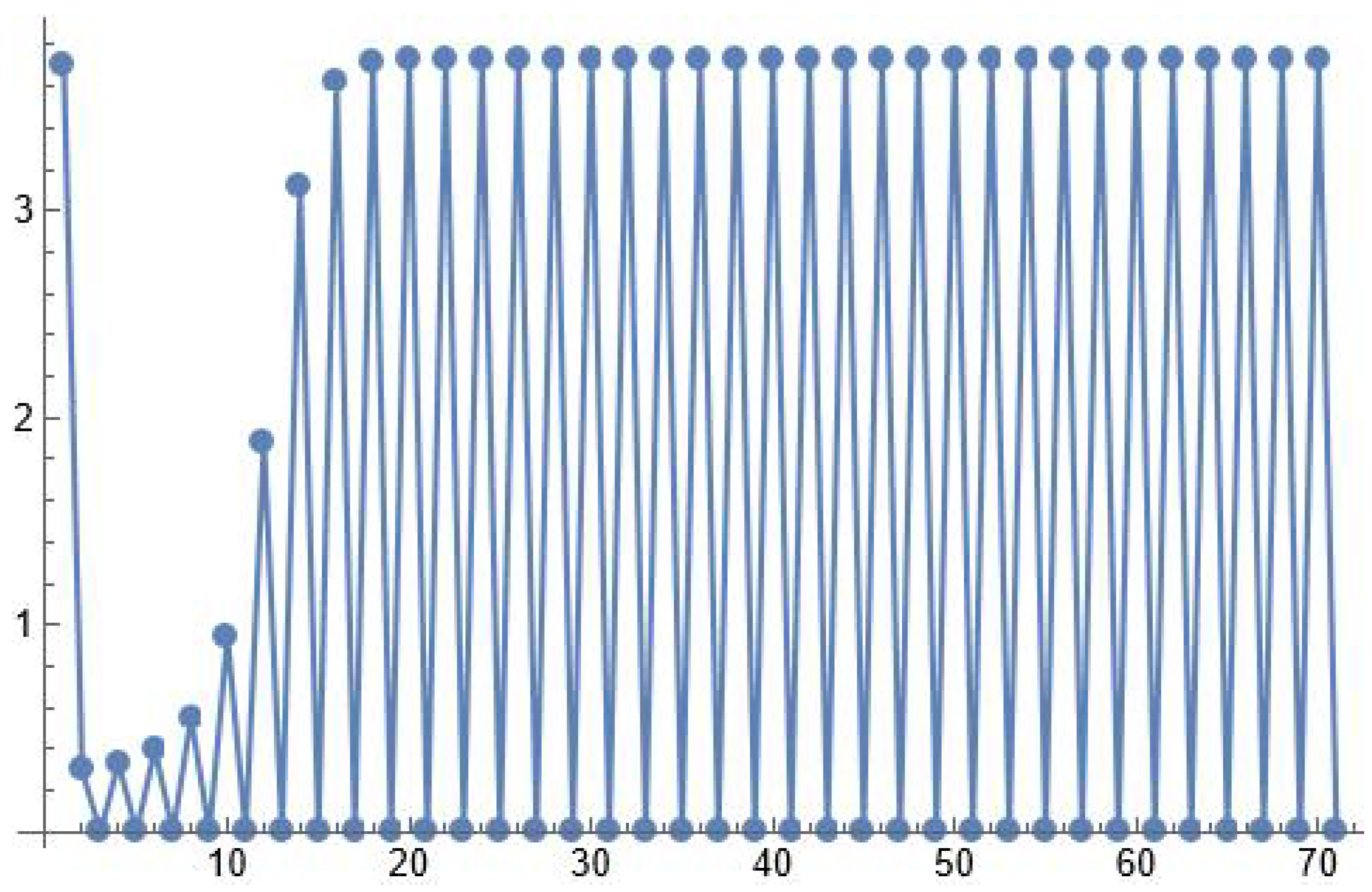
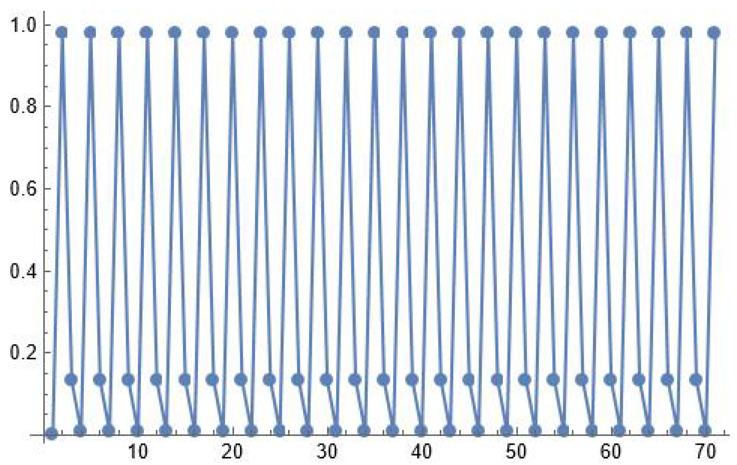
See Figure 3 for visual illustration of convergence to the period-two solution and Figure 4 for visual illustrations of convergence to the period-three solution.

Theorem 11.

The boundary $\partial B\left(p\right)$ of the basin of attraction for Equation (1) is a continuous manifold consisting of non-comparable points, which contains all periodic solutions and the equilibrium solution $E_{-}({\overline{x}}_{-},{\overline{x}}_{-},{\overline{x}}_{-})$ and its Lipschitz surface.

Proof. 

It follows from Theorem 3 and the observaton that $T^3$ is strongly cooperative map, given that T is a cooperative map. □

6. Discussion

The sigmoid Beverton Holt difference equation of second order, which is Equation (2), serves as a basic model in population dynamics. This second-order equation is the simplest known model that involves two interesting scenarios: Allee’s effect (species extinction) and convergence to either an equilibrium solution or to both some equilibrium solutions and period-two solutions; see [1,2,5]. Dynamics of third-order equation (16) is characterized by a large number of the period-three solutions. Dynamics of Equation (1) is an interaction of dynamics of these two equations and so, if $a_1+a_2$ dominates $a_3$, it should be expected that the resulting dynamics of Equation (1) is similar to the dynamics of Equation (2). If $a_1+a_2$ is dominated by $a_3$, it should be expected that resulting dynamics of Equation (1) has a number of period-three solutions outside of the basins of attraction of the equilibrium solutions. We showed this to be true with some examples. An interesting case for further study is the case when $a_1+a_2$ and $a_3$ are balanced. What kind of dynamics holds, then? Furthermore, when a general difference equation of third order, where function f is non-decreasing in all arguments (5), does it exhibit chaos? What are the additional conditions on f that will imply that the existence of period-three solution implies chaos?

7. Conclusions

In this paper, local and global dynamics of Equation (1) are investigated, from the point of determining the basins of attraction of different equilibrium points. The techniques based on component-wise monotonicity of transition function and on theory of monotone operators were used to give the description of the basins of attraction of different equilibrium points. Equation (2) has relatively simple behavior, where all solutions converge to either equilibrium solutions or to period-two solutions. In addition, the basins of attraction of all equilibrium solutions or period-two solutions of Equation (2) are separated by the global stable manifolds of neighboring equilibrium solutions or period-two solutions, which are saddle points. This dynamic behavior is precisely described in [1]. We generalized the result on global stable manifold of saddle point to be the separatrix between two basins of attraction of neighboring locally stable equilibrium points to a higher dimensional case (see [23]), and we applied this result to Equation (1). In general, the set that separates the two basins of attraction of locally stable equilibrium points should contain different periodic points. Introduction of a third term $x_{n-2}$ changes dynamics dramatically as a variety of period-three solutions appear even in the very special case of Equation (16). The resulting dynamics of Equation (1) is the combination of these two different dynamics, when one of two equations Equation (2) and Equation (16) dominates. The interesting case for future research is the dynamics in the case when the coefficients $a_1+a_2$ and $a_3$ are balanced. Another interesting problem is possible appearance of chaos in the presence of period-three solutions.

References

1. Bilgin, A.; Kulenović, M.R.S.; Pilav, E. Basins of Attraction of Period-Two Solutions of Monotone Difference Equations. Adv. Differ. Equ. 2016, 2016, 25. [Google Scholar] [CrossRef]
2. Allen, L. An Introduction to Mathematical Biology; Pearson: Boston, MA, USA, 2006. [Google Scholar]
3. Thieme, H.R. Mathematics in Population Biology; Princeton Series in Theoretical and Computational Biology; Princeton University Press: Princeton, NJ, USA, 2003; xx+543p. [Google Scholar]
4. Camouzis, E.; Ladas, G. Dynamics of Third-Order Rational Difference Equations with Open Problems and Conjectures; Advances in Discrete Mathematics and Applications; Chapman & Hall/CRC: Boca Raton, FL, USA, 2008; Volume 5. [Google Scholar]
5. Elaydi, S.N.; Cushing, J.M. Discrete Mathematical Models in Population Biology–Ecological, Epidemic, and Evolutionary Dynamics; Springer Undergraduate Texts in Mathematics and Technology; Springer: Cham, Switzerland, 2024; xiv+481p. [Google Scholar]
6. Camouzis, E.; Ladas, G.; Quinn, E.P. On third-order rational difference equations. II. J. Differ. Equ. Appl. 2004, 10, 1041–1047. [Google Scholar]
7. Camouzis, E.; Chatterjee, E.; Ladas, G.; Quinn, E.P. On third-order rational difference equations. III. J. Difference Equ. Appl. 2004, 12, 1119–1127. [Google Scholar]
8. Camouzis, E.; Ladas, G. On third-order rational difference equations. V. J. Differ. Equ. Appl. 2005, 11, 553–562. [Google Scholar] [CrossRef]
9. Camouzis, E.; Ladas, G.; Quinn, E.P. On third-order rational difference equations. VI. J. Differ. Equ. Appl. 2005, 11, 759–777. [Google Scholar] [CrossRef]
10. Camouzis, E.; Ladas, G. On third-order rational difference equations. I. J. Difference Equ. Appl. 2008, 14, 333–343. [Google Scholar]
11. Kulenović, M.R.S.; Nurkanović, Z. Global behavior of a three-dimensional linear fractional system of difference equations. J. Math. Anal. Appl. 2005, 310, 673–689. [Google Scholar] [CrossRef]
12. Hess, P. Periodic-Parabolic Boundary Value Problems and Positivity; Pitman Research Notes in Mathematics Series; Longman Scientific and Technical, Harlow; John Wiley and Sons, Inc.: New York, NY, USA, 1991; Volume 247. [Google Scholar]
13. Hirsch, M.W.; Smith, H. Competitive and Cooperative Systems: Mini-Review. In Positive Systems (Rome, 2003); Lecture Notes in Control and Information Science; Springer: Berlin/Heidelberg, Germany, 2003; Volume 294, pp. 183–190. [Google Scholar]
14. Hirsch, M.W.; Smith, H. Monotone maps: A review. J. Differ. Equ. Appl. 2005, 11, 379–398. [Google Scholar] [CrossRef]
15. Hirsch, M.W.; Smith, H. Monotone Dynamical Systems. In Handbook of Differential Equations: Ordinary Differential Equations; Elsevier B.V.: Amsterdam, The Netherlands, 2005; Volume II, pp. 239–357. [Google Scholar]
16. Cima, A.; Gasull, A.; Manosa, V. Asymptotic Stability for Block Triangular Maps. Sarajevo J. Math. 2022, 18, 25–44. [Google Scholar] [CrossRef]
17. Elaydi, S. An Introduction to Difference Equations, 3rd ed.; Springer: New York, NY, USA, 2005. [Google Scholar]
18. Hale, J.K.; Kocak, H. Dynamics and Bifurcations; Texts in Applied Mathematics; Springer: New York, NY, USA, 1991; Volume 3. [Google Scholar]
19. Kocić, V.; Ladas, G. Global Behavior of Nonlinear Difference Equations of Higher Order with Applications; Mathematics and its Applications; Kluwer Academic Publishers Group: Dordrecht, The Switzerland, 1993; Volume 256. [Google Scholar]
20. Lakshmikantham, V.; Trigiante, D. Theory of Difference Equations: Numerical Methods and Applications, 2nd ed.; Monographs and Textbooks in Pure and Applied Mathematics; Marcel Dekker, Inc.: New York, NY, USA, 2002; Volume 251. [Google Scholar]
21. Robinson, C. Stability, Symbolic Dynamics, and Chaos; CRC Press: Boca Raton, FL, USA, 1995. [Google Scholar]
22. Wiggins, S. Introduction to Applied Nonlinear Dynamical Systems and Chaos, 2nd ed.; Texts in Applied Mathematics; Springer: New York, NY, USA, 2003; Volume 2. [Google Scholar]
23. Kulenović, M.R.S.; Marcotte, J.; Merino, O. Cones for Coordinate-wise Monotone Functions and Dynamics of Monotone Maps. J. Differ. Equ. Appl. 2025. submitted. [Google Scholar]
24. Janowski, E.J.; Kulenović, M.R.S. Attractivity and global stability for linearizable difference equations. Comput. Math. Appl. 2009, 57, 1592–1607. [Google Scholar] [CrossRef]
25. Cushing, J.M. An evolutionary Beverton-Holt model. In Theory and Applications of Difference Equations and Discrete Dynamical Systems; Springer Proc. Math. Stat., 102; Springer: Berlin/Heidelberg, Germany, 2014; pp. 127–141. [Google Scholar]
26. Cushing, J.M. One Dimensional Maps as Population and Evolutionary Dynamic Models. In Applied Analysis in Biological and Physical Sciences; Springer Proceedings in Mathematics & Statistics; Springer: New Delhi, India, 2016; Volume 186, pp. 41–62. [Google Scholar]
27. Cushing, J.M. Difference equations as models of evolutionary population dynamics. J. Biol. Dyn. 2019, 13, 103–127. [Google Scholar] [CrossRef] [PubMed]
28. Clark, C.W. A delayed recruitment model of population dynamics with an application to baleen whale populations. J. Math. Biol. 1976, 3, 381–391. [Google Scholar] [CrossRef] [PubMed]
Figure 1. Basins of attraction of period-three points of Equation (16) with a 3 = 3 . The boxes with different colors represent the parts of the basins of attraction of two locally stable equilibrium points and two locally stable period-three points. The boundary surface between different basins of attraction is complicated. The surfaces are ploted in 3 D coordinate system in the box [ 0 , 2 ] 3 .
Mathematics 13 02990 g001
Figure 2. Basins of attraction of two locally stable equilibrium solutions of Equation (16) with a 1 = 0 , a 2 = 2 , a 3 = 1 . In the absence of the periodic points, the boundary surface between different basins of attraction is simpler. The surfaces are ploted in 3 D coordinate system in the box [ 0 , 2 ] 3 .
Mathematics 13 02990 g002
Figure 3. First 70 terms of the solution of x n + 1 = 0.01 x n 2 1 + x n 2 + 4 x n 1 2 1 + x n 1 2 + 0.04 x n 2 2 1 + x n 2 2 with x 0 = 3.7 , x 1 = 0.7 , x 2 = 0 as a time series plot. The horizontal axis stands for n and the vertical axis stands for x n . The solution converges to period-two solution { 0.00475552 , 3.73205 } .
Mathematics 13 02990 g003
Figure 4. First 70 terms of the solution of x n + 1 = 0.2 x n 2 1 + x n 2 + 0.01 x n 1 2 1 + x n 1 2 + 2 x n 2 2 1 + x n 2 2 with x 0 = 0.001 , x 1 = 0.98 , x 2 = 0.132 . as a time series plot. The horizontal axis stands for n and the vertical axis stands for x n . The solution converges to period-three solution { 0.00850314 , 0.980645 , 0.132609 } .
Mathematics 13 02990 g004
Disclaimer/Publisher’s Note: The statements, opinions and data contained in all publications are solely those of the individual author(s) and contributor(s) and not of MDPI and/or the editor(s). MDPI and/or the editor(s) disclaim responsibility for any injury to people or property resulting from any ideas, methods, instructions or products referred to in the content.