Abstract
This article addresses a two-dimensional inverse problem of magnetotelluric sounding under the assumption of E-polarized electromagnetic fields. The main focus is on the construction of a forward numerical model based on the Helmholtz equation with a complex coefficient, and the recovery of electrical conductivity from boundary measurements. The second-order finite difference method is employed for numerical simulation, providing stable approximations of both the direct and the conjugate problems. The inverse problem is formulated as a minimization of a data misfit functional, and solved using Nesterov’s accelerated gradient descent method, which ensures fast convergence and robustness to noise. Numerical experiments are presented for a synthetic model featuring a smooth background conductivity and a localized anomaly. Comparison between the exact and reconstructed solutions demonstrates the high accuracy and efficiency of the proposed algorithm. The developed approach can serve as a foundation for constructing practical inversion schemes in geophysical exploration problems.
Keywords:
Helmholtz equation; magnetotelluric sounding; inverse problem; Nesterov method; numerical solution MSC:
35Q86; 35R30; 65N12
1. Introduction
The magnetotelluric (MT) method is one of the most informative and widely used techniques in electromagnetic geophysical exploration. It enables the investigation of the Earth’s crustal structure at considerable depths. The method is based on the use of natural variations of the electromagnetic field resulting from the solar wind and the Earth’s magnetosphere. By measuring the electric and magnetic field components at the surface, it becomes possible to reconstruct the distribution of subsurface electrical properties, such as electrical conductivity [1,2,3].
The MT method is extensively applied in geophysics to address problems related to the investigation of the deep structure of the lithosphere, the detection of geothermal anomalies, the assessment of mineral and hydrocarbon resources, as well as the monitoring of active faults and seismically active zones [4,5]. Due to its high sensitivity to both vertical and horizontal inhomogeneities, the method enables the construction of geoelectrical cross-sections in geologically complex environments, making it a vital tool in both practical exploration and scientific research.
From a mathematical point of view, the modeling and inversion of magnetotelluric data are based on the Maxwell system of equations, which in the case of E-polarization reduces to the Helmholtz equation with a complex coefficient. This formulation takes into account the frequency-dependent conductivity of the medium and allows the application of advanced numerical methods for elliptical problems. Therefore, the Helmholtz equation serves as a convenient and rigorous mathematical basis for solving direct and inverse MTZ problems [1].
The magnetotelluric (MT) method has long been recognized as one of the most powerful tools in electromagnetic geophysics, providing information on the Earth’s lithosphere and crustal structures at great depths. Foundational works such as Berdichevsky and Dmitriev [1] established the theoretical and methodological framework of MT, while later studies emphasized the challenges of interpreting layered or finely heterogeneous media [6]. Laboratory and experimental studies further demonstrated the sensitivity of MT data to temperature, pressure, and mineral composition, thus highlighting the complexity of linking field measurements to geoelectrical models [7]. A recent review by Lin et al. [8] summarized a wide variety of subsurface conductivity anomalies observed in MT imaging, underlining the continuing importance of reliable inversion techniques.
Despite the maturity of the MT method, solving its inverse problem remains highly challenging. Quasi-one-dimensional approaches [9] and optimization-based two-dimensional methods [10] have been developed to improve stability, yet they often suffer from reduced accuracy or heavy computational costs. The inclusion of borehole constraints [11] or joint inversion with passive seismic data [12] demonstrated improved resolution, but at the expense of increased methodological complexity. Practical developments, such as the use of SEP acquisition systems [13] or the integration of infrared remote sensing [14], illustrated the benefits of hybrid exploration strategies, but they do not fully resolve the inherent instability of the inverse problem. From a mathematical perspective, classical formulations of the inverse Helmholtz problem [15,16,17] showed that ill-posedness and sensitivity to noise are fundamental obstacles, reinforcing the need for efficient and stable inversion schemes.
Recent advances point toward two promising directions. First, there is a renewed interest in coefficient inverse problems for the Helmholtz equation, where conductivity is treated as a spatially varying complex parameter [18]. Second, the integration of physics-driven machine learning has opened up new opportunities for MT inversion: Liu et al. [19] proposed a deep learning framework constrained by physical laws, while Deng et al. [20] developed neural-network-based forward modeling with applications to inversion. These works highlight the demand for methods that combine mathematical rigor with computational efficiency.
The present article is focused on the numerical modeling and solution of the two-dimensional inverse magnetotelluric problem under E-polarization. The proposed approach is based on a variational formulation involving the Helmholtz equation with a complex coefficient that describes the spatially varying electrical conductivity of the medium. Second-order finite difference schemes are employed for numerical computations, and the inverse problem is formulated as an optimization task using Nesterov’s accelerated gradient method. This approach ensures stability, convergence, and accuracy of parameter reconstruction, making it an effective tool for interpreting electromagnetic data in geophysical applications.
2. Materials and Methods
Impedance and its Tensor Formulation. Impedance is a central concept in magnetotelluric sounding, enabling the transition from the measured components of the electric and magnetic fields to a quantitative characterization of the geoelectrical medium. In the most general case, when the conductivity of the medium depends on spatial coordinates (in two- or three-dimensional models), the simple scalar definition of impedance becomes insufficient. In such cases, the impedance tensor is introduced [1].
Scalar Form (1D Model):
In the case of a horizontally homogeneous (1D) medium, impedance is defined as the ratio of the corresponding components of the electric and magnetic fields:
When the electric field is oriented along the -axis and the magnetic field along the -axis:
When the electric field is oriented along the -axis and the magnetic field along the -axis:
here:
- −
- —components of the horizontal electric field;
- −
- —components of the horizontal magnetic field;
Tensor Form (2D and 3D Models):
In more complex, heterogeneous media, impedance is described by a complex second-rank tensor:
- −
- —components of the impedance tensor (complex quantities with units of Ohms), which depend on frequency and the geographic location of the measurement.
The components of the impedance tensor contain information about the structural anisotropy of the medium, the presence of lateral inhomogeneities, and the geometry of subsurface layers. In two-dimensional models, the approximation is often valid, leaving only and , which significantly simplifies the interpretation [1].
Analysis of the impedance tensor components’ magnitudes plays a key role in magnetotelluric investigations. It enables the identification of the direction of maximum conductivity in the medium, the separation of regional and local geoelectrical anomalies, as well as the calculation of apparent resistivity and phases, which are used in inversion procedures. Moreover, impedance diagrams constructed from tensor components are employed in the visual interpretation of field data. Thus, the tensor formulation of impedance is an essential element of modern magnetotelluric interpretation and is necessary for analyzing complex geological structures in two- and three-dimensional models.
Problem Statement. In this study, a two-dimensional inverse magnetotelluric problem is considered under the assumption of E-polarized electromagnetic fields. The primary objective is to reconstruct the spatial distribution of electrical conductivity from the known impedance measured at the Earth’s surface. The forward problem is formulated as a Helmholtz equation with a complex coefficient and appropriate boundary conditions. The inverse problem is solved using a gradient-based method formulated as a minimization of a misfit functional.
Let us consider the formulation of the two-dimensional inverse magnetotelluric problem in the case of E-polarized electromagnetic fields [1,6,9]. Assume that the electrical conductivity in the lower half-space (for ) is distributed as follows:
Let us consider a two-dimensional MT model in the case of E-polarization of the electromagnetic field. It is assumed that the electric field is directed along the -axis, while the medium’s conductivity depends on the coordinates and . Differentiation with respect to the -axis is absent: .
In the forward problem, the electric field satisfies the following Helmholtz equation:
On the lateral boundaries (left and right), boundary values corresponding to the normal (background) model of the field are imposed:
At the upper boundary , a radiation excitation condition is imposed:
At the lower boundary , an absorbing (outgoing wave) boundary condition is applied:
where —wave number in air (above the model),
- —wave number in the deep layer of the model,
- —amplitude of the incident (exciting) external field.
- —is the normal field that describes the behavior of the electric field in the case of a one-dimensional model and is defined as the solution to the following one-dimensional boundary value problem:
After solving Equation (6) with boundary conditions (7)–(9), the impedance at the surface is computed as:
Let us introduce the following notations for simplification:
Then the problem takes the following form:
The domain considered in this problem is shown in Figure 1.
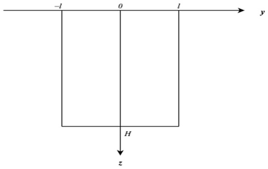
Figure 1.
Domain of the Helmholtz equation.
Generalized Solution of the Two-Dimensional MT Problem. In problems with coefficients depending on multiple variables and involving complex-valued quantities, the solution may lack classical second-order derivatives. In such cases, the concept of a generalized solution in Sobolev spaces is employed [21,22].
Definition 1.
the following integral identity holds
A function is called a generalized solution of the direct problem (14)–(17) if for any test function satisfying the following conditions:
The existence and a priori estimate of the generalized solution to the two-dimensional problem (14)–(17) are established in Theorem 1. Similar results have also been obtained in studies [21,22].
Theorem 1.
Let the coefficient and the parameters . Then there exists a unique generalized solution satisfying the weak formulation (21), and this solution satisfies the following a priori estimate:
where the constant depends only on the dimensions of the domain the norm , and the coefficients .
Let us consider the formulation of the direct and inverse problems. In the direct problem (14)–(17), the goal is to find given the functions . In the inverse problem, the aim is to determine based on additional information
The direct problem, formulated by equations (14)–(17), describes the distribution of the complex electric field in a geoelectric medium with a given parameter associated with conductivity. It is known that the parameter of the medium directly depends on the conductivity distribution and must be reconstructed based on experimentally measured data.
The goal of the inverse problem is to reconstruct the parameter from known values of the impedance , measured at the boundary . To achieve this, a misfit functional is introduced:
where is the impedance obtained from observational data, and is the solution to the direct problem for a given distribution of the parameter . We now derive the variation of the functional [22,23,24]:
Let us introduce the substitution:
We obtain the following expression:
We formulate the perturbed problem:
Subtracting problem (14)–(17) from problem (24)–(27), we obtain the problem for
Let us consider the identically zero expression derived from (28), and integrate it by parts to obtain:
Using (29), (30), and (31), we obtain
On the other hand, the variation of the functional can be directly expressed as:
From this follows the formulation of the adjoint problem
We obtain the expression
We obtain the expression for the gradient of the functional
where is the solution of the adjoint problem (32)–(35).
Numerical Solution of the One-Dimensional Problem. To specify the boundary values for the two-dimensional model, an auxiliary one-dimensional problem is used, describing the vertical behavior of the electric field in a one-dimensional medium. This model is referred to as the normal (background) model and is intended to approximate the electromagnetic field in the case when the conductivity of the medium depends only on depth , i.e., , without accounting for horizontal inhomogeneity. We solve the numerical one-dimensional problem (9)–(11) in order to obtain the lateral boundary conditions for Equations (14)–(17).
where . Introducing the following notations the one-dimensional problem can be written in the following form
The domain is divided into uniform intervals with step size:
After introducing the variables and discretizing the domain on a uniform grid, a second-order finite difference scheme was derived to approximate the one-dimensional boundary value problem describing the normal electromagnetic field [23,24].
After obtaining the finite difference form of the one-dimensional normal electromagnetic field equation, the problem reduces to solving a linear system with a tridiagonal matrix. The Thomas algorithm (also known as the tridiagonal matrix algorithm) is employed for its numerical solution.
Numerical solution of the two-dimensional problem. To numerically solve both the forward and the adjoint problems, a second-order finite difference method is used, providing a balanced combination of implementation simplicity and sufficient approximation accuracy. A direct method, described in detail in [23,24,25], is employed to solve the resulting discrete system.
For efficient numerical solution of the inverse problem using the gradient descent method, it is necessary to compute the gradient of the misfit functional. This, in turn, requires solving the adjoint problem, which is formulated as a second-order linear elliptic differential equation with appropriate boundary conditions.
where .
The combination of the discretized internal equations and boundary conditions forms a complete system of linear algebraic equations to be solved for each value of the frequency . Solving the adjoint problem is necessary for computing the gradient of the misfit functional in the iterative process of reconstructing the coefficient , making the developed scheme a key component of the inverse problem algorithm.
Inverse Problem Algorithm Based on Nesterov’s Method. For the numerical solution of the inverse problem, it is formulated as an optimization problem in which a specifically defined objective functional is minimized. The efficiency and convergence of the solution largely depend on the choice of the optimization method. In this study, Nesterov’s method is employed, which has proven to be one of the fastest and most robust gradient-based techniques. This approach features a high convergence rate and provides accelerated convergence compared to classical gradient descent, which is particularly important when solving computationally intensive problems arising in magnetotelluric inversion [22].
In the accelerated gradient method of Nesterov, the step size is usually chosen as , where is the Lipschitz constant of the gradient of the objective functional [26]. The gradient of the functional is said to be -Lipschitz continuous if, for any , the following inequality holds:
where is the smallest constant satisfying this condition. In both the gradient descent method and Nesterov’s method, the step size α\alphaα is chosen such that
which guarantees a decrease of the functional and convergence of the algorithm. Intuitively, limits the “steepness” of the gradient change: the larger , the smaller the step size must be in order to avoid overshooting the minimum. In our computations, the value of was assigned in advance and refined empirically to ensure stable convergence.
As a stopping criterion, in the case of exact (noise-free) data, we use the decrease of the functional:
where is a prescribed accuracy threshold [21].
To implement Nesterov’s method, we set the following parameters: , where is the Lipschitz constant of the gradient.
- Choose an initial approximation and assign
- Solve the direct problem (43)–(46) numerically for ;
- Compute the value of the functional using Formula (23);
- If the value of the objective functional is not sufficiently small, solve the adjoint problem (47)–(50)
- Compute the gradient of the functional using Formula (36);
- Compute the first approximation ;
- Assuming that are known, compute the parameters
- Compute ;
- Solve the direct problem (43)–(46) numerically for ;
- Compute the value of the functional ;
- If the value of the objective functional is not sufficiently small, solve the adjoint problem (47)–(50)
- Compute the gradient of the functional ;
- Compute the next approximation and return to step 7;
3. Results
Numerical Modeling Results. To evaluate the efficiency of the proposed numerical algorithm, a two-dimensional model of electrical conductivity , was constructed, which includes a background distribution and a localized Gaussian anomaly. The background part of the model depends only on depth and is described by the function , while the anomaly is introduced in the central region of the modeling domain and has spatial localization in both and directions.
At the first stage, a one-dimensional problem was solved for the normal field , which is used as the boundary condition on the lateral sides of the two-dimensional domain. The obtained solution agrees with the expected behavior of the electromagnetic field in a stratified medium.
At the second stage, a complete two-dimensional system of linear algebraic equations (SLAE) was constructed, corresponding to the approximation of the Helmholtz equation with a variable complex coefficient . The system was solved using the sparse matrix method.
Parameters of the Numerical Experiment. In the numerical experiment, a two-dimensional model with a Gaussian conductivity anomaly located in a bounded region was used. The horizontal half-width of the modeling dom1ain is , and the depth of the domain is . The frequency range is defined in the interval from 1 to 10 with a step of 0.2, , and the angular frequency is calculated using the formula .
The anomalous conductivity is defined by a Gaussian function:
The background (normal) conductivity distribution with depth is described by the expression:
The air conductivity is assumed to be , and at the lower boundary of the domain . The magnetic permeability of the medium is considered constant throughout the entire domain and equal to . The amplitude of the excitation field (the virtual source) is normalized to .
In Figure 2a the real part of the field exhibits smooth spatial variations: the values are maximal in the central part of the domain and gradually decrease toward the edges. This distribution reflects the influence of the central conductive anomaly and the symmetry of the geoelectric structure along the -axis.

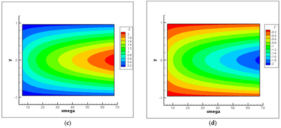
Figure 2.
Numerical solution of the direct problem with the given model parameters: (a) real part of the electromagnetic field ; (b) imaginary part of the electromagnetic field ; (c) real part of the impedance as a function of y and frequency ; (d) imaginary part of the impedance as a function of y and frequency .
In Figure 2b the imaginary part of the field shows a less symmetric pattern with a pronounced minimum in the center and more complex gradients. This behavior is associated with phase effects and the sensitivity of the imaginary component to deep conductivity heterogeneities.
Both components of the field exhibit correct behavior and serve as the basis for further analysis of the impedance and reconstruction of the subsurface structure.
Additionally, Figure 2 presents the plots of the real (c) and imaginary (d) parts of the impedance as functions of frequency and horizontal coordinate .
In Figure 2c the real part of the impedance shows a pronounced maximum in the central part of the domain (near ) and decreases toward the edges (). As the frequency increases, there is a general decrease in the values of , which corresponds to the reduced penetration depth of the electromagnetic field. This pattern may be attributed to a localized conductivity anomaly in the center of the domain.
Figure 2d the imaginary part of the impedance—also exhibits characteristic behavior: near the center the values are most negative, while they increase toward zero at the edges. This indicates a phase shift between the electric and magnetic fields, which intensifies in regions of higher conductivity. Similar to the real part, an increase in frequency leads to a reduction in the amplitude of oscillations.
Both components of the impedance are sensitive to horizontal inhomogeneities of the medium and clearly reflect the presence of a conductive structure in the central region. This confirms the high informativeness of the impedance tensor in frequency-spatial analysis of magnetotelluric data.
Figure 3 presents the results of the numerical solution of the two-dimensional inverse magnetotelluric problem obtained using Nesterov’s method. The comparison is made between the exact conductivity distribution and the approximate solution obtained after a finite number of iterations. The top part of the figure (a and b) shows the exact solution in two-dimensional and three-dimensional visualizations, respectively. It represents a smooth, symmetric structure with a maximum in the center and a gradual decrease in values toward the boundaries of the domain.
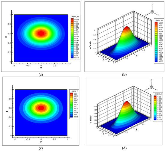
Figure 3.
Graphical comparison of exact and reconstructed electrical conductivity distributions: (a) exact conductivity in the 2D model; (b) exact conductivity in the 3D model; (c) reconstructed conductivity in the 2D model; (d) reconstructed conductivity in the 3D model.
The bottom part of the figure (c and d) illustrates the approximate solution reconstructed using Nesterov’s method. It can be seen that the recovered distribution closely replicates the shape and amplitude of the exact solution. The center of the maximum coincides with the exact location, and the contours retain a smooth and symmetric structure. The largest deviations between the exact and approximate solutions are observed in regions with high conductivity values, where the problem becomes more sensitive to data inaccuracies and iterative errors. This is explained by the enhanced influence of such areas on the behavior of the wave field, as well as increased nonlinearity in these zones.
4. Discussion
Figure 4 presents the numerical results of solving the inverse magnetotelluric problem obtained using the Nesterov method and, for comparison, the Landweber method. Figure 4a,b show the convergence curves of the objective functional . The Nesterov method demonstrates significantly faster convergence: the value of the functional reaches the level of within only 35 iterations, while the Landweber method requires more than 80 iterations to achieve comparable accuracy. The reduction in iteration count directly translates into lower computational cost, which emphasizes the advantage of the accelerated gradient approach compared with traditional iterative schemes.
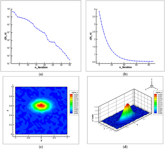
Figure 4.
Numerical results of solving the inverse magnetotelluric problem. (a) convergence curve of the objective functional using the Nesterov method; (b) convergence curve of the objective functional using the Landweber method; (c) reconstructed distribution of the function ) in 2D using the Landweber method; (d) reconstructed distribution of the function ) in 3D using the Landweber method.
Figure 4c,d illustrate the reconstructed conductivity distribution . Visual comparison with the true Gaussian anomaly confirms that the Nesterov method successfully recovers the main structure with higher accuracy than the Landweber method. To further strengthen the evaluation, future experiments are planned with more complex scenarios, including multiple anomalies, noisy data, and irregular boundaries. In this model problem, an exponential function was chosen as a test example, since the recovery of such functions is traditionally considered a considerable challenge in inverse problems. Future studies will also employ real data and more complex anomalies. The present article is primarily aimed at demonstrating the methodology for solving inverse problems of magnetotelluric sounding.
Thus, the obtained results show that the accelerated gradient method of Nesterov not only improves the rate of convergence but also provides high accuracy in reconstructing conductivity distributions in MT inversion problems, confirming its potential as a competitive alternative to standard optimization methods.
5. Conclusions
In this study, a two-dimensional inverse magnetotelluric (MT) problem under E-polarization was investigated. The research has a review-applied character and focuses on constructing a forward numerical model of the electromagnetic response of a geoelectrical medium. The modeling is based on the Helmholtz equation with a complex coefficient, where the medium’s conductivity varies both with depth and along the transverse coordinate.
A synthetic model was constructed for the numerical experiment, incorporating a smooth background conductivity and a localized conductive anomaly. The computed electromagnetic field and surface impedance demonstrated high sensitivity to medium inhomogeneities. The observed symmetry in the field and local maxima in the impedance confirm the correctness of the numerical algorithm.
Furthermore, the inverse problem of recovering the conductivity distribution from synthetic data was solved using Nesterov’s method, known for its accelerated convergence. The numerical experiment showed that even with limited information, it is possible to achieve high reconstruction accuracy, with the cost functional reaching its minimum value within a limited number of iterations. The obtained approximate solution closely matches the original model, confirming the efficiency and practical applicability of the proposed approach.
Thus, the results of this work demonstrate that the proposed numerical scheme and inversion algorithm are suitable both for forward modeling and for reliable solution of inverse MT problems, making them promising tools for geophysical interpretation.
Author Contributions
Conceptualization, N.M.T. and S.E.K.; methodology, A.M.T. and N.M.T.; software M.N.D., Z.G.T. and Z.S.T.; validation, Z.G.T. and Z.S.T.; formal analysis, A.N.T. and S.E.K.; writing—original draft preparation, M.N.D.; writing—review and editing, A.M.T. and S.E.K. All authors have read and agreed to the published version of the manuscript.
Funding
The research is funded by Science Committee of the Ministry of Science and Higher Education of the Republic of Kazakhstan (Grant No. BR27100483 “Development of predictive exploration technologies for identifying ore-prospective areas based on data analysis from the unified subsurface user platform “Minerals.gov.kz” using artificial intelligence and remote sensing methods”).
Data Availability Statement
The original contributions presented in this study are included in the article material. Further inquiries can be directed to the corresponding authors.
Conflicts of Interest
The authors declare no conflict of interest.
References
- Berdichevsky, M.N.; Dmitriev, V.I. Models and Methods of Magnetotellurics; Springer Science & Business Media: Berlin/Heidelberg, Germany, 2008. [Google Scholar]
- Vozoff, K. The magnetotelluric method. In Electromagnetic Methods in Applied Geophysics: Volume 2, Application, Parts A and B; Nabighian, M.N., Corbett, J.D., Eds.; Society of Exploration Geophysicists: Houston, TX, USA, 1991. [Google Scholar] [CrossRef]
- Simpson, F.; Bahr, K. Practical Magnetotellurics; Cambridge University Press: Cambridge, UK, 2005. [Google Scholar] [CrossRef]
- Unsworth, M. Magnetotelluric Studies of Lithospheric Structure Beneath Western Canada: Insights into Plate Tectonics Both Past and Present; Department of physics, University of Alberta: Edmonton, AB, Canada, 2015; pp. 28–32. [Google Scholar]
- Egbert, G.D.; Kelbert, A. Computational recipes for electromagnetic inverse problems. Geophys. J. Int. 2012, 189, 251–267. [Google Scholar] [CrossRef]
- Dmitriev, V.I. Magnetotelluric sounding of a layered medium containing thin inhomogeneous layers. Comput. Math. Model. 2018, 29, 127–133. (In Russian) [Google Scholar]
- Pommier, A. Interpretation of magnetotelluric results using laboratory measurements. Surv. Geophys. 2014, 35, 41–84. [Google Scholar] [CrossRef]
- Lin, W.; Yang, B.; Han, B.; Hu, X. A review of subsurface electrical conductivity anomalies in magnetotelluric imaging. Sensors 2023, 23, 1803. [Google Scholar] [CrossRef] [PubMed]
- Berezina, N.I.; Dmitriev, V.I.; Mershchikova, N.A. A quasi-one-dimensional method for solving a two-dimensional inverse problem of magnetotelluric sounding. Appl. Math. Comput. Sci. 2010, 5–16. Available online: https://cs.msu.ru/sites/cmc/files/docs/berezinadmitrievmershchikova_t.35.pdf (accessed on 29 July 2025). (In Russian).
- Van Beusekom, A.E.; Parker, R.L.; Bank, R.E.; Gill, P.E.; Constable, S. The 2-D magnetotelluric inverse problem solved with optimization. Geophys. J. Int. 2011, 184, 639–650. [Google Scholar] [CrossRef]
- Kalscheuer, T.; Juhojuntti, N.; Vaittinen, K. Two-dimensional magnetotelluric modelling of ore deposits: Improvements in model constraints by inclusion of borehole measurements. Surv. Geophys. 2018, 39, 467–507. [Google Scholar] [CrossRef]
- Gabàs, A.; Macau, A.; Benjumea, B.; Queralt, P.; Ledo, J.; Figueras, S.; Marcuello, A. Joint audio-magnetotelluric and passive seismic imaging of the Cerdanya Basin. Surv. Geophys. 2016, 37, 897–921. [Google Scholar] [CrossRef]
- Di, Q.; Xue, G.; Zeng, Q.; Wang, Z.; An, Z. Magnetotelluric exploration of deep-seated gold deposits in the Qingchengzi orefield, Eastern Liaoning (China), using a SEP system. Ore Geol. Rev. 2020, 122, 103501. [Google Scholar] [CrossRef]
- Chen, H.; Xie, X.; Liu, E.; Zhou, L.; Yan, L. Application of infrared remote sensing and magnetotelluric technology in geothermal resource exploration: A case article of the wuerhe area, Xinjiang. Remote Sens. 2021, 13, 4989. [Google Scholar] [CrossRef]
- Magnanini, R.; Papi, G. An inverse problem for the Helmholtz equation. Inverse Probl. 1985, 1, 357. [Google Scholar] [CrossRef]
- Angell, T.S.; Kleinman, R.E.; Roach, G.F. An inverse transmission problem for the Helmholtz equation. Inverse Probl. 1987, 3, 149. [Google Scholar] [CrossRef]
- Tadi, M.; Nandakumaran, A.K.; Sritharan, S.S. An inverse problem for Helmholtz equation. Inverse Probl. Sci. Eng. 2011, 19, 839–854. [Google Scholar] [CrossRef]
- Sibiryakov, E.B. Coefficient inverse problem for the Helmholtz equation. Geophys. Technol. 2023, 77–84. [Google Scholar] [CrossRef]
- Liu, W.; Wang, H.; Xi, Z.; Zhang, R.; Huang, X. Physics-driven deep learning inversion with application to magnetotelluric. Remote Sens. 2022, 14, 3218. [Google Scholar] [CrossRef]
- Deng, F.; Hu, J.; Wang, X.; Yu, S.; Zhang, B.; Li, S.; Li, X. Magnetotelluric deep learning forward modeling and its application in inversion. Remote Sens. 2023, 15, 3667. [Google Scholar] [CrossRef]
- Kabanikhin, S.I. Inverse and Ill-Posed Problems: Theory and Applications; de Gruyter: Berlin, Germany, 2011. [Google Scholar] [CrossRef]
- Kasenov, S.E.; Tleulesova, A.M.; Temirbekov, A.N.; Bektemessov, Z.M.; Asanova, R.A. Numerical Solution of the Inverse Thermoacoustics Problem Using QFT and Gradient Method. Fractal Fract. 2025, 9, 370. [Google Scholar] [CrossRef]
- Kasenov, S.E.; Demeubayeva, Z.E.; Temirbekov, N.M.; Temirbekova, L.N. Solution of the Optimization Problem of Magnetotelluric Sounding in Quaternions by the Differential Evolution Method. Computation 2024, 12, 127. [Google Scholar] [CrossRef]
- Temirbekov, N.; Temirbekov, A.; Kasenov, S.; Tamabay, D. Numerical modeling for enhanced pollutant transport prediction in industrial atmospheric air. Int. J. Des. Nat. Ecodynamics 2024, 19, 917–926. [Google Scholar] [CrossRef]
- Samarsky, A.A.; Gulin, A.V. Numerical Methods; Nauka: Moscow, Russia, 1989; 432p. (In Russian) [Google Scholar]
- Nesterov, Y. A method for solving the convex programming problem with convergence rate O (1/k2). Dokl. Akad. Nauk. Sssr 1983, 269, 543. Available online: https://www.mathnet.ru/links/a11843a16f534bd95b16c6df52aec0fd/dan46009.pdf (accessed on 5 September 2025). (In Russian).


Disclaimer/Publisher’s Note: The statements, opinions and data contained in all publications are solely those of the individual author(s) and contributor(s) and not of MDPI and/or the editor(s). MDPI and/or the editor(s) disclaim responsibility for any injury to people or property resulting from any ideas, methods, instructions or products referred to in the content. |
© 2025 by the authors. Licensee MDPI, Basel, Switzerland. This article is an open access article distributed under the terms and conditions of the Creative Commons Attribution (CC BY) license (https://creativecommons.org/licenses/by/4.0/).